MOOSE Workshop
July 2026
Idaho National Laboratory
www.inl.gov
Established in 2005, INL is the lead nuclear energy R&D laboratory for the Department of Energy
"Establish a world-class capability in the modeling and simulation of advanced energy systems..."
INL is the one of the largest employers in Idaho with over 6,000 employees and 500 interns
In 2024 the INL budget was over $2 billion
INL is the site where 52 nuclear reactors were designed and constructed, including the first reactor to generate usable amounts of electricity: Experimental Breeder Reactor I (EBR-1)

Advanced Test Reactor (ATR)
World's most powerful test reactor (250 MW thermal)
Constructed in 1967
Volume of 1.4 cubic meters, with 43 kg of uranium, and operates at 60C

Transient Reactor Test Facility (TREAT)
TREAT is a test facility specifically designed to evaluate the response of fuels and materials to accident conditions
High-intensity (20 GW), short-duration (80 ms) neutron pulses for severe accident testing
National Reactor Innovation Center (NRIC)
NRIC is composed of two physical test beds to build prototypes of advanced nuclear reactors:
DOME (Demonstration of Microreactor Experiments) in the historic EBR-II facility, a test bed site capable of hosting operational nuclear reactor concepts that produce less than 20MW thermal power.
LOTUS (Laboratory for Operation and Testing in the U.S.) in the historic Zero Power Physics Reactor (ZPPR) Cell, a test bed site capable of hosting operational nuclear reactor concepts that produce less than 500kW thermal power.
NRIC also manages the open-source Virtual Test Bed to demonstrate advanced reactors through modeling and simulation. More information about NRIC can be found at https://nric.inl.gov.
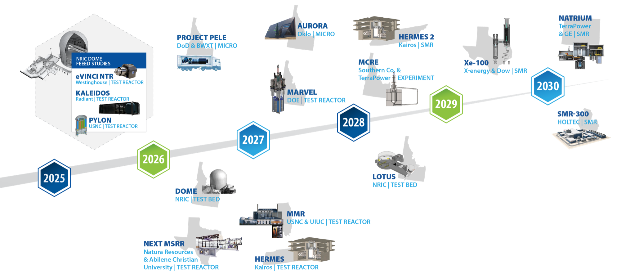
Advanced Reactor Demonstration Timeline
MOOSE
Multi-physics Object Oriented Simulation Environment
mooseframework.inl.gov

History and Purpose
Development started in 2008
Open-sourced in 2014
Designed to solve computational engineering problems and reduce the expense and time required to develop new applications by:
Being easily extended and maintained
Working efficiently on a few and many processors
Providing an object-oriented, extensible system for creating all aspects of a simulation tool
Motivated by multiphysics problems in nuclear engineering, but applications have extended into diverse fields
Core team at Idaho National Laboratory, but with significant contributions from other laboratories, universities, and industry, both domestically and internationally
By The Numbers
250 contributors
58,000 commits
5,000 unique visitors per month
~40 new Discussion participants per week
150M tests per week
General Capabilities
Continuous and Discontinuous Galerkin FEM
Finite Volume
Supports fully coupled or segregated systems, fully implicit and explicit time integration
Automatic differentiation (AD)
Unstructured mesh with FEM shapes
Higher order geometry
Mesh adaptivity (refinement and coarsening)
Massively parallel (MPI and threads)
User code agnostic of dimension, parallelism, shape functions, etc.
Native support for executing multiphysics simulations across applications
GPU support for execution via MFEM and Kokkos
Operating Systems:
macOS (Conda, Docker)
Linux (Apptainer, Conda, Docker)
Windows (Docker, WSL)
Object-oriented, pluggable system

Example Code
Software Quality
Follows a Nuclear Quality Assurance Level 1 (NQA-1) development process
All changes undergo independent review and must pass regression tests before merge
Includes a test suite and documentation system to allow for agile development while maintaining a NQA-1 process
External contributions are guided through the process by the team, and are very welcome!
Development Process

Community
github.com/idaholab/moose/discussions

License
LGPL 2.1
Does not limit what you can do with your application
Can license/sell your application as closed source
Modifications to the library itself (or the modules) are open source
New contributions are automatically LGPL 2.1
Multiphysics Simulation
Historical Multiphysics Simulation
Predictive multiphysics capability involved best-estimate calculations
Best estimates: data and correlation driven, many approximations
Necessitated experimental data for each design
Physics performed independently
Was a "siloed" task; handoffs of data/results from person to person
While individual codes were computationally efficient and well validated, coupling them was neither efficient nor well validated
Used many approximations for evaluations of safety parameters
Pin-power reconstruction, gap conductance, spacer grid models
Modern Multiphysics Simulation
Direct, physics-based models of all components
Reduces approximations as needed
Can be computationally expensive
Can employ tighter and more consistent coupling
Length and time scales of physics can be vastly different
What does this change for the analyst?
Not as well validated:
Experiments prohibitively expensive
Very large design space
Modularity is Key
Data should be accessed through strict interfaces with code having separation of responsibilities
Allows for "decoupling" of code
Leads to more reuse and less bugs
Challenging for FEM
Shape functions, degrees of freedom, meshing, quadrature points, material properties, analytic functions, global integrals, data transfer, ...
The complexity makes computational science codes brittle and hard to reuse
A consistent set of "systems" are needed to carry out common actions, these systems should be separated by interfaces
Finite-Element Reactor Fuel Simulation
MOOSE Coupling Strategies
Coupling strategies:
Full coupling: Solve all physics in a single (linear or nonlinear) system
Loose coupling: Solve each physics sequentially
Tight coupling: Solve each physics sequentially and iterate
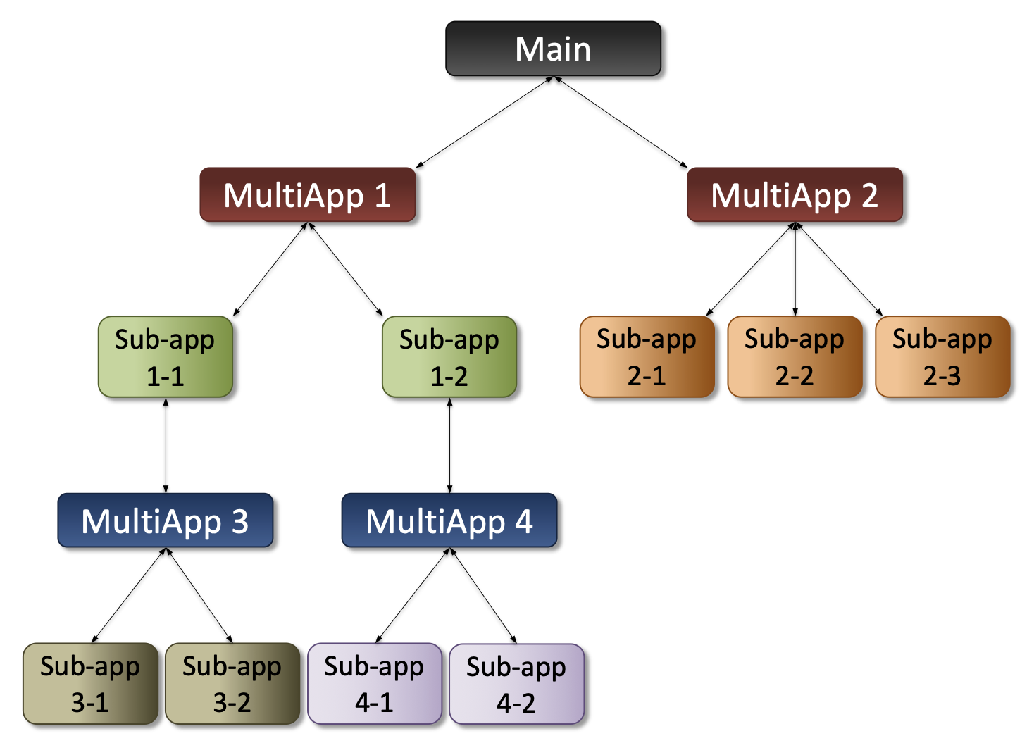
Segregated (loose/tight) coupling achieved using
MultiAppsPhysics coupled via in-memory transfer of fields and scalars
Coupling specified in the input file (no code needed)
No universally superior coupling strategy; correct choice depends on problem
Provides a standardized interface for an analyst to produce a coupled model
MOOSE MultiApp Hierarchy Example
Getting started
Required for upcoming hands-on
Installing a text editor with input file syntax auto-complete
Problem Statement
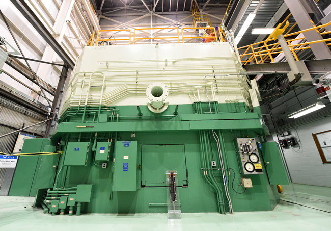
We will study the cooling of the concrete shielding around a future micro-reactor in the DOME Test Bed at the National Reactor Innovation Center in Idaho.
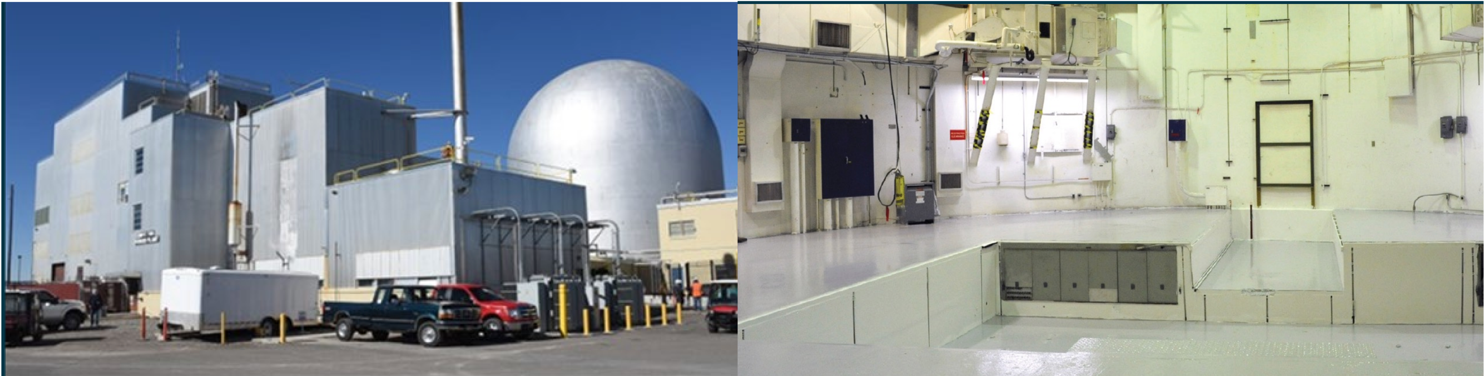
Exterior (left), Interior (right)
This example was created independently from studies at NRIC and INL. The dimensions have been modified and numerous systems and complexities are omitted.
Cooling system schematic (from NRIC overview Nov. 21)
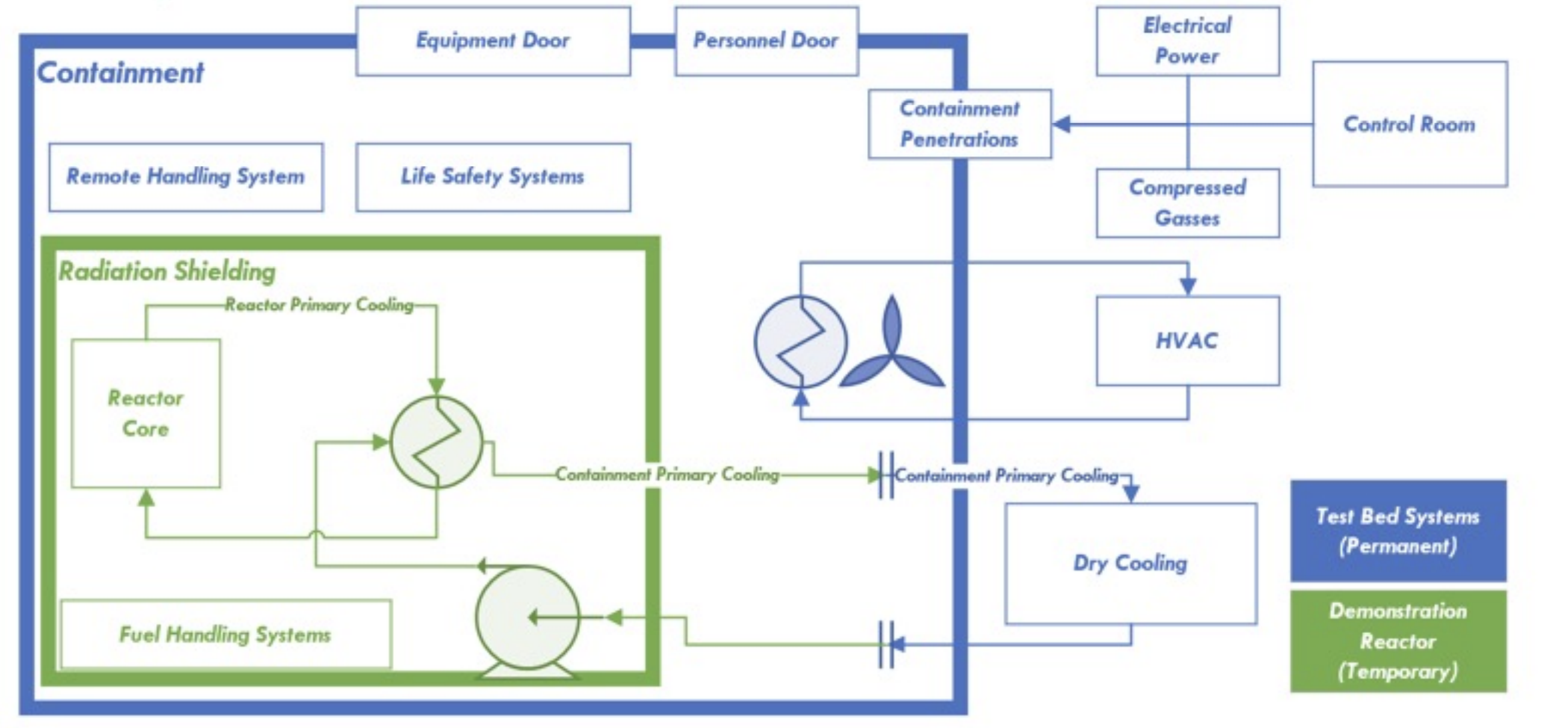
Simplified geometry:
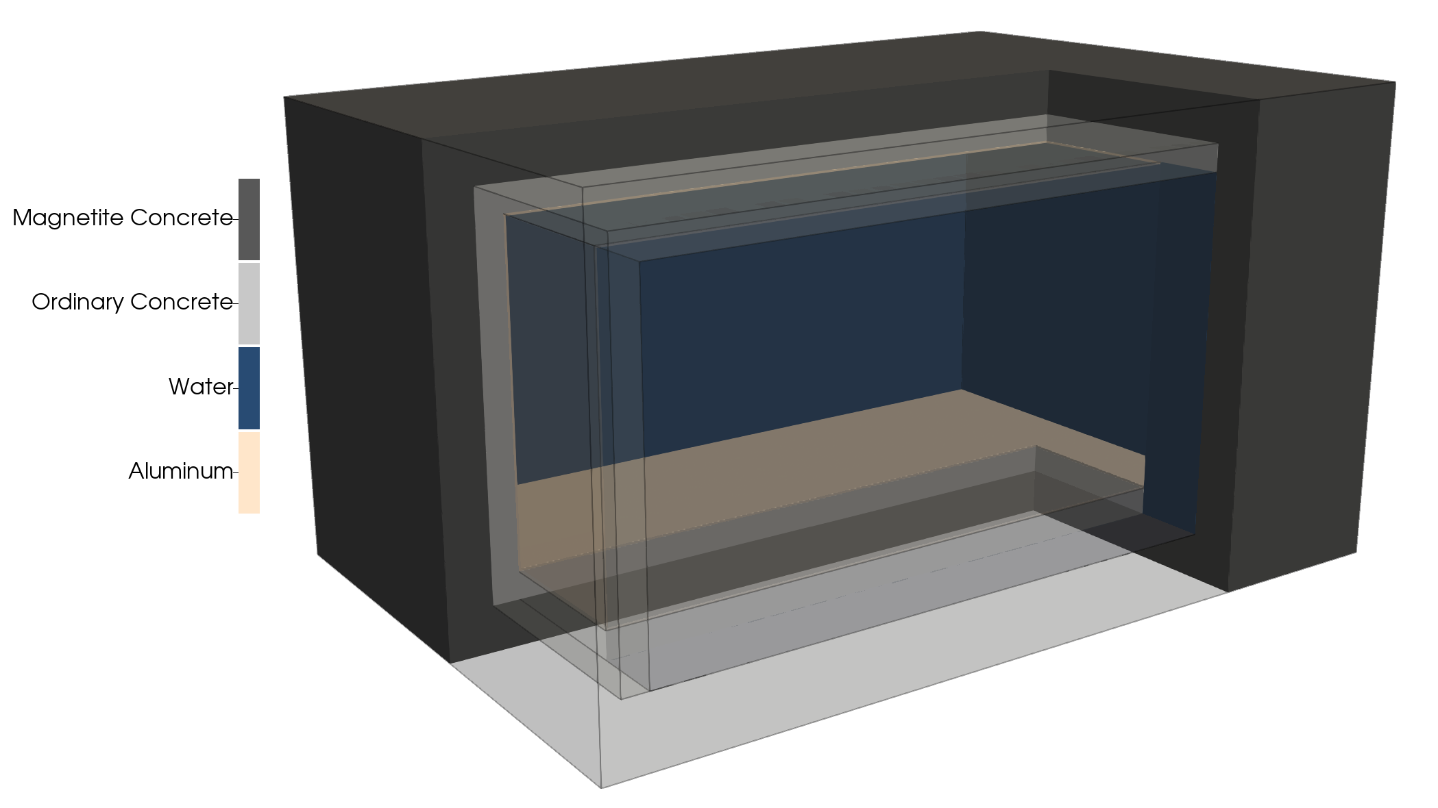
6.5m x 9.7m x 5.25m concrete box with 4m x 7.6m x 3.6m room
Physics of Interest
Concrete Domain: Thermal Mechanics
Heat conduction of the thermal radiation from the reactor to the boundary of shield.
Mechanical displacement and stress from the thermal expansion.
Water Domain: Thermal Fluids
Heat transfer through the fluid and back-and-forth from the concrete.
Natural convection of the fluid due to the temperature gradients.
Material Properties
| Property | Units | Magnetite Concrete | Ordinary Concrete | Aluminum | Water |
|---|---|---|---|---|---|
| Thermal conductivity, | W/(mK) | 5.0 | 2.25 | 175 | 0.6 |
| Density, | kg/m | 3,524 | 2,403 | 2,270 | 955.7 |
| Heat capacity, | J/(kgK) | 1,050 | 1,050 | 875 | 4,181 |
| Viscosity, | mPas | — | — | — | 0.798 |
| Water heat transfer coefficient | W/m K | 600 | 600 | 600 | — |
| Air heat transfer coefficient | W/m K | 10 | — | — | — |
| Young's modulus | GPa | 2.75 | 30 | 68 | — |
| Poisson's ratio | — | 0.15 | 0.2 | 0.36 | |
| Thermal expansion coefficient | 10/K | 1.0 | 1.0 | 2.4 | — |
Tutorial Steps
Step 1: Geometry and Diffusion
Step 2: Simple Heat Conduction Kernel
Step 3: Boundary conditions
Step 4: Heat Conduction kernel with Material
Step 5: Auxiliary Variables
Step 6: Transient Heat Conduction
Step 7: Mechanics
Step 8: Mesh Adaptivity
Step 9: Postprocessors
Step 10: Finite Volume
Step 11: Multiscale Simulation
Step 12: Custom Syntax
Step 13: Recover, restart and initialization hands-on
Step 1: Geometry and Diffusion
The first step is to solve a simple "Diffusion" problem. This step will introduce the basic system of MOOSE.
Step 2: Simple Heat Conduction Kernel
In order to implement the heat conduction equation, a Kernel object is needed to represent:
Step 3: Boundary conditions
We represent the boundary conditions using BC objects. For example, Dirichlet boundary conditions:
Neumann boundary conditions:
or convective boundary conditions:
Step 4: Heat Conduction kernel with Material
Instead of passing constant parameters to the heat conduction Kernel object, the Material system can be used to supply the values. This allows for properties that vary in space and time as well as be coupled to variables in the simulation.
Step 5: Auxiliary Variables
The heat flux can be compute from the temperature as:
This velocity can be computed using the Auxiliary system.
Step 6: Transient Heat Conduction
Solve the transient heat equation using the "heat transfer" module.
Step 7: Mechanics
Thermal expansion of the concrete can be added to the coupled set of equations using the "solid mechanics" module.
Step 8: Mesh Adaptivity
In the transient simulation, a "traveling wave" profile moves through the concrete as it heats up. Adaptivity lets us resolve the temperature gradient at lower computational cost.
Step 9: Postprocessors
Postprocessor and VectorPostprocessor objects can be used to compute aggregate value(s) for a simulation, such as the average temperature on the boundary or the temperatures along a line within the solution domain.
Step 10: Finite Volume
Solve the pressure, velocity and temperature in a coupled system of equations by solving for heat transfer in the fluid region
Conservation of Mass (incompressible):
Conservation of momentum:
Conservation of Energy:
Step 11: Multiscale Simulation
MOOSE is capable of running multiple applications together and transfer data between the various applications.
We introduce distributed thermal calculations for neutron detectors, placing the detectors in various locations in the concrete.
Step 12: Custom Syntax
MOOSE includes a system to create custom input syntax for common tasks, in this step the syntax for the sets of equations are simplified for end-users.
Step 13: Recover, restart and initialization hands-on
Learn how to recover a MOOSE simulation that ended prematurely.
MOOSE Input File Syntax
MOOSE uses WASP, developed at Oak Ridge National Laboratory, to process input files. Input files use a hierarchical syntax, with square brackets [something] to delineate levels.
                       # These are comments
[Variables]            # system name
  [u]                  # object name, opening sub-block
    family = LAGRANGE  # a parameter for this object
    order = FIRST      # another parameter for this object
  []                   # closing object sub-block
[]                     # closing system block
More info on input syntax on this page.
Comments
Comments are preceded by #. They are ignored by the input file parsing. They can be written on their own line:
# Let's define some variables!
[Variables]
  ...
or after valid syntax:
[Variables]  # Let's define some variables!
  ...
Mesh System
A system for defining a finite element / volume mesh.
Creating a Mesh
For complicated geometries, we often use CUBIT from Sandia National Laboratories cubit.sandia.gov.
Other mesh generators can work as long as they output a file format that libMesh reads.
Mesh generators
Meshes in MOOSE are built or loaded using MeshGenerators.
To only generate the mesh without running the simulation, you can pass --mesh-only on the command line.
FileMeshGenerator
FileMeshGenerator is the MeshGenerator to load external meshes:
[Mesh]
  [fmg]
    type = FileMeshGenerator
    file = square.exo
  []
[]
MOOSE supports reading and writing a large number of formats and could be extended to read more.
| Extension | Description |
|---|---|
| .dat | Tecplot ASCII file |
| .e, .exo | Sandia's ExodusII format |
| .fro | ACDL's surface triangulation file |
| .gmv | LANL's GMV (General Mesh Viewer) format |
| .mat | Matlab triangular ASCII file (read only) |
| .msh | GMSH ASCII file |
| .n, .nem | Sandia's Nemesis format |
| .plt | Tecplot binary file (write only) |
| .node, .ele; .poly | TetGen ASCII file (read; write) |
| .inp | Abaqus .inp format (read only) |
| .ucd | AVS's ASCII UCD format |
| .unv | I-deas Universal format |
| .xda, .xdr | libMesh formats |
| .vtk, .pvtu | Visualization Toolkit |
Generating Meshes in MOOSE
Built-in mesh generation is implemented for lines, rectangles, or extruded reactor geometries.
[Mesh]
  [generated]
    type = GeneratedMeshGenerator
    dim = 2
    xmin = 0
    xmax = 1
    nx = 2
    ymin = -2
    ymax = 3
    ny = 3
    elem_type = 'TRI3'
  []
[]
The sides are named in a logical way and are numbered:
1D: left = 0, right = 1
2D: bottom = 0, right = 1, top = 2, left = 3
3D: back = 0, bottom = 1, right = 2, top = 3, left = 4, front = 5
The capability is very convenient for parametric mesh optimization!
Named Entity Support
Human-readable names can be assigned to blocks, sidesets, and nodesets that can be used throughout an input file.
A parameter that requires an ID will accept either numbers or "names".
Names can be assigned to IDs for existing meshes to ease input file maintenance.
We create a mesh with ids, and give the blocks, identified by their id, names for convenience
[Mesh]
  [bulk]
    type = CartesianMeshGenerator
    dim = 3
    dx = '0.5 0.75 0.025 4.0 0.025 0.75 0.5'
    dy = '0.5 0.3 0.025 7.6 0.025 0.75 0.5'
    dz = '0.5 0.3 0.025 3.6 0.025 0.3 0.5'
    ix = '2 3 1 16 1 3 2'
    iy = '2 1 1 30 1 3 2'
    iz = '2 1 1 14 1 1 2'
    subdomain_id = '
      0 0 0 0 0 0 0
      0 0 0 0 0 0 0
      0 0 0 0 0 0 0
      0 0 0 0 0 0 0
      0 0 0 0 0 0 0
      0 0 0 0 0 0 0
      0 0 0 0 0 0 0

      0 0 0 0 0 0 0
      0 1 1 1 1 1 0
      0 2 2 1 2 2 0
      0 2 2 1 2 2 0
      0 2 2 2 2 2 0
      0 2 2 2 2 2 0
      0 0 0 0 0 0 0

      0 0 0 0 0 0 0
      0 1 1 1 1 1 0
      0 2 2 3 2 2 0
      0 2 2 3 2 2 0
      0 2 2 2 2 2 0
      0 2 2 2 2 2 0
      0 0 0 0 0 0 0

      0 0 0 0 0 0 0
      0 1 1 1 1 1 0
      0 2 2 3 2 2 0
      0 2 2 4 2 2 0
      0 2 2 2 2 2 0
      0 2 2 2 2 2 0
      0 0 0 0 0 0 0

      0 0 0 0 0 0 0
      0 1 1 1 1 1 0
      0 2 2 3 2 2 0
      0 2 2 3 2 2 0
      0 2 2 2 2 2 0
      0 2 2 2 2 2 0
      0 0 0 0 0 0 0

      0 0 0 0 0 0 0
      0 1 1 1 1 1 0
      0 1 1 1 1 1 0
      0 1 1 1 1 1 0
      0 1 1 1 1 1 0
      0 1 1 1 1 1 0
      0 0 0 0 0 0 0

      0 0 0 0 0 0 0
      0 0 0 0 0 0 0
      0 0 0 0 0 0 0
      0 0 0 0 0 0 0
      0 0 0 0 0 0 0
      0 0 0 0 0 0 0
      0 0 0 0 0 0 0
      '
  []
  [rename_blocks]
    type = RenameBlockGenerator
    input = hollow_concrete
    old_block = '0 1 2 3'
    new_block = 'concrete_hd concrete water Al'
    show_info = true
  []
[]
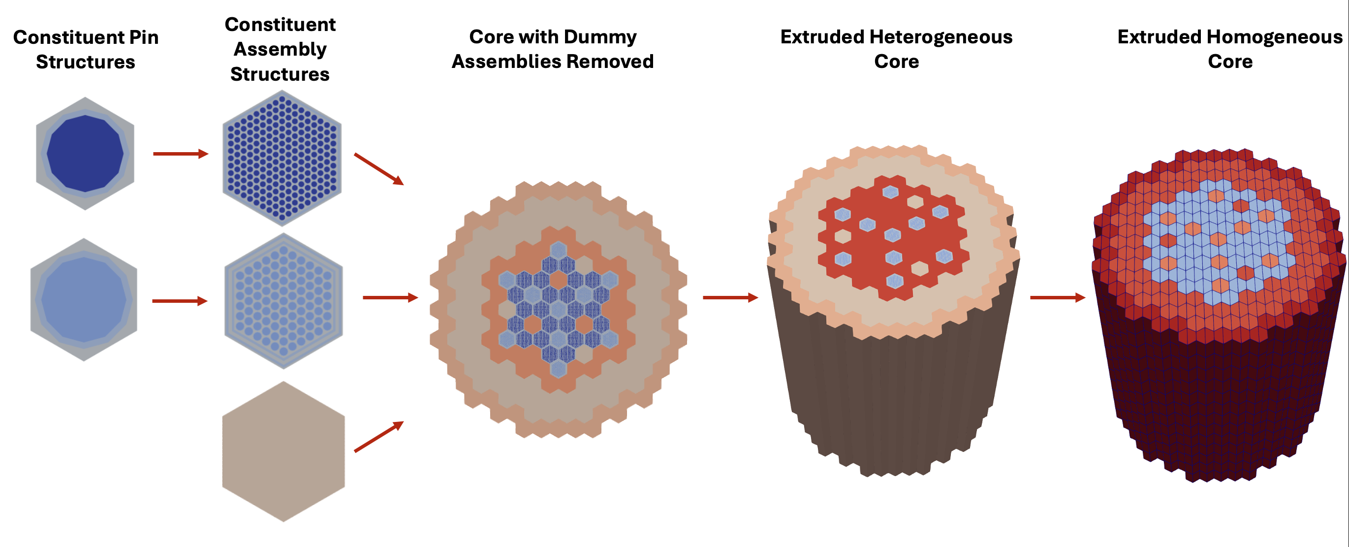
Chaining mesh operations
We can chain the generation of unit cell meshes, stitching to form lattices, extrusion and homogenization to form this advanced reactor mesh, entirely using MOOSE mesh generators.
Step 1: Geometry and Diffusion
Mesh Generation
Meshes can be generated in MOOSE using mesh generators.
2D slice of the shield domain using GeneratedMeshGenerator:
[Mesh]
  [bulk]
    type = GeneratedMeshGenerator
    dim = 2
    xmax = 6.5
    ymax = 9.7
    nx = 7
    ny = 10
  []
[]
An executable is available from loading the MOOSE conda or HPC module.
cd ~/projects/moose/tutorials/shield_multiphysics/inputs/step01_diffusion
moose-opt -i mesh_part1.i --mesh-only
Console output in mesh-only mode shows a summary of the mesh.
 Mesh Information:
  elem_dimensions()={2}
  elem_default_orders()={FIRST}
  supported_nodal_order()=1
  spatial_dimension()=2
  n_nodes()=88
    n_local_nodes()=88
  n_elem()=70
    n_local_elem()=70
    n_active_elem()=70
  n_subdomains()=1
  n_elemsets()=0
  n_partitions()=1
  n_processors()=1
  n_threads()=1
  processor_id()=0
  is_prepared()=true
  is_replicated()=true

 Mesh Bounding Box:
  Minimum: (x,y,z)=(       0,        0,        0)
  Maximum: (x,y,z)=(     6.5,      9.7,        0)
  Delta:   (x,y,z)=(     6.5,      9.7,        0)

 Mesh Element Type(s):
  QUAD4

 Mesh Nodesets:
  Nodeset 0 (bottom), 8 nodes
   Bounding box minimum: (x,y,z)=(       0,        0,        0)
   Bounding box maximum: (x,y,z)=(     6.5,        0,        0)
   Bounding box delta: (x,y,z)=(     6.5,        0,        0)
  Nodeset 1 (right), 11 nodes
   Bounding box minimum: (x,y,z)=(     6.5,        0,        0)
   Bounding box maximum: (x,y,z)=(     6.5,      9.7,        0)
   Bounding box delta: (x,y,z)=(       0,      9.7,        0)
  Nodeset 2 (top), 8 nodes
   Bounding box minimum: (x,y,z)=(       0,      9.7,        0)
   Bounding box maximum: (x,y,z)=(     6.5,      9.7,        0)
   Bounding box delta: (x,y,z)=(     6.5,        0,        0)
  Nodeset 3 (left), 11 nodes
   Bounding box minimum: (x,y,z)=(       0,        0,        0)
   Bounding box maximum: (x,y,z)=(       0,      9.7,        0)
   Bounding box delta: (x,y,z)=(       0,      9.7,        0)

 Mesh Sidesets:
  Sideset 0 (bottom), 7 sides (EDGE2), 7 elems (QUAD4), 8 nodes
   Side volume: 6.5
   Bounding box minimum: (x,y,z)=(       0,        0,        0)
   Bounding box maximum: (x,y,z)=(     6.5,        0,        0)
   Bounding box delta: (x,y,z)=(     6.5,        0,        0)
  Sideset 1 (right), 10 sides (EDGE2), 10 elems (QUAD4), 11 nodes
   Side volume: 9.7
   Bounding box minimum: (x,y,z)=(     6.5,        0,        0)
   Bounding box maximum: (x,y,z)=(     6.5,      9.7,        0)
   Bounding box delta: (x,y,z)=(       0,      9.7,        0)
  Sideset 2 (top), 7 sides (EDGE2), 7 elems (QUAD4), 8 nodes
   Side volume: 6.5
   Bounding box minimum: (x,y,z)=(       0,      9.7,        0)
   Bounding box maximum: (x,y,z)=(     6.5,      9.7,        0)
   Bounding box delta: (x,y,z)=(     6.5,        0,        0)
  Sideset 3 (left), 10 sides (EDGE2), 10 elems (QUAD4), 11 nodes
   Side volume: 9.7
   Bounding box minimum: (x,y,z)=(       0,        0,        0)
   Bounding box maximum: (x,y,z)=(       0,      9.7,        0)
   Bounding box delta: (x,y,z)=(       0,      9.7,        0)

 Mesh Edgesets:
  None

 Mesh Subdomains:
  Subdomain 0: 70 elems (QUAD4, 70 active), 88 active nodes
   Volume: 63.05
   Bounding box minimum: (x,y,z)=(       0,        0,        0)
   Bounding box maximum: (x,y,z)=(     6.5,      9.7,        0)
   Bounding box delta: (x,y,z)=(     6.5,      9.7,        0)
  Global mesh volume = 63.05
Capturing features of the geometry using CartesianMeshGenerator:
 @@ -1,10 +1,10 @@
 [Mesh]
   [bulk]
-    type = GeneratedMeshGenerator
+    type = CartesianMeshGenerator
     dim = 2
-    xmax = 6.5
-    ymax = 9.7
-    nx = 7
-    ny = 10
+    dx = '0.5 0.75 0.025 4.0 0.025 0.75 0.5'
+    dy = '0.5 0.3 0.025 7.6 0.025 0.75 0.5'
+    ix = '2 3 1 16 1 3 2'
+    iy = '2 1 1 30 1 3 2'
   []
 []
(+ tutorials/shield_multiphysics/inputs/step01_diffusion/mesh_part2.i)

Specifying subdomains or "blocks" to capture differing materials:
 @@ -1,10 +1,17 @@
 [Mesh]
   [bulk]
     type = CartesianMeshGenerator
     dim = 2
     dx = '0.5 0.75 0.025 4.0 0.025 0.75 0.5'
     dy = '0.5 0.3 0.025 7.6 0.025 0.75 0.5'
     ix = '2 3 1 16 1 3 2'
     iy = '2 1 1 30 1 3 2'
+    subdomain_id = '0 0 0 0 0 0 0
+                    0 1 1 1 1 1 0
+                    0 2 2 3 2 2 0
+                    0 2 2 4 2 2 0
+                    0 2 2 2 2 2 0
+                    0 2 2 2 2 2 0
+                    0 0 0 0 0 0 0'
   []
 []
(+ tutorials/shield_multiphysics/inputs/step01_diffusion/mesh_part3.i)
Extending to 3D with "slices" of the domain:
 @@ -1,17 +1,69 @@
 [Mesh]
   [bulk]
     type = CartesianMeshGenerator
-    dim = 2
+    dim = 3
     dx = '0.5 0.75 0.025 4.0 0.025 0.75 0.5'
     dy = '0.5 0.3 0.025 7.6 0.025 0.75 0.5'
+    dz = '0.5 0.3 0.025 3.6 0.025 0.3 0.5'
     ix = '2 3 1 16 1 3 2'
     iy = '2 1 1 30 1 3 2'
-    subdomain_id = '0 0 0 0 0 0 0
-                    0 1 1 1 1 1 0
-                    0 2 2 3 2 2 0
-                    0 2 2 4 2 2 0
-                    0 2 2 2 2 2 0
-                    0 2 2 2 2 2 0
-                    0 0 0 0 0 0 0'
+    iz = '2 1 1 14 1 1 2'
+    subdomain_id = '
+      0 0 0 0 0 0 0
+      0 0 0 0 0 0 0
+      0 0 0 0 0 0 0
+      0 0 0 0 0 0 0
+      0 0 0 0 0 0 0
+      0 0 0 0 0 0 0
+      0 0 0 0 0 0 0
+
+      0 0 0 0 0 0 0
+      0 1 1 1 1 1 0
+      0 2 2 1 2 2 0
+      0 2 2 1 2 2 0
+      0 2 2 2 2 2 0
+      0 2 2 2 2 2 0
+      0 0 0 0 0 0 0
+
+      0 0 0 0 0 0 0
+      0 1 1 1 1 1 0
+      0 2 2 3 2 2 0
+      0 2 2 3 2 2 0
+      0 2 2 2 2 2 0
+      0 2 2 2 2 2 0
+      0 0 0 0 0 0 0
+
+      0 0 0 0 0 0 0
+      0 1 1 1 1 1 0
+      0 2 2 3 2 2 0
+      0 2 2 4 2 2 0
+      0 2 2 2 2 2 0
+      0 2 2 2 2 2 0
+      0 0 0 0 0 0 0
+
+      0 0 0 0 0 0 0
+      0 1 1 1 1 1 0
+      0 2 2 3 2 2 0
+      0 2 2 3 2 2 0
+      0 2 2 2 2 2 0
+      0 2 2 2 2 2 0
+      0 0 0 0 0 0 0
+
+      0 0 0 0 0 0 0
+      0 1 1 1 1 1 0
+      0 1 1 1 1 1 0
+      0 1 1 1 1 1 0
+      0 1 1 1 1 1 0
+      0 1 1 1 1 1 0
+      0 0 0 0 0 0 0
+
+      0 0 0 0 0 0 0
+      0 0 0 0 0 0 0
+      0 0 0 0 0 0 0
+      0 0 0 0 0 0 0
+      0 0 0 0 0 0 0
+      0 0 0 0 0 0 0
+      0 0 0 0 0 0 0
+      '
   []
 []
(+ tutorials/shield_multiphysics/inputs/step01_diffusion/mesh_part4.i)
Z-axis not to scale
Finally, we can string together mesh generators to:
Remove blocks with BlockDeletionGenerator
Rename blocks to something more memorable with RenameBlockGenerator
 @@ -1,69 +1,101 @@
 [Mesh]
   [bulk]
     type = CartesianMeshGenerator
     dim = 3
     dx = '0.5 0.75 0.025 4.0 0.025 0.75 0.5'
     dy = '0.5 0.3 0.025 7.6 0.025 0.75 0.5'
     dz = '0.5 0.3 0.025 3.6 0.025 0.3 0.5'
     ix = '2 3 1 16 1 3 2'
     iy = '2 1 1 30 1 3 2'
     iz = '2 1 1 14 1 1 2'
     subdomain_id = '
       0 0 0 0 0 0 0
       0 0 0 0 0 0 0
       0 0 0 0 0 0 0
       0 0 0 0 0 0 0
       0 0 0 0 0 0 0
       0 0 0 0 0 0 0
       0 0 0 0 0 0 0

       0 0 0 0 0 0 0
       0 1 1 1 1 1 0
       0 2 2 1 2 2 0
       0 2 2 1 2 2 0
       0 2 2 2 2 2 0
       0 2 2 2 2 2 0
       0 0 0 0 0 0 0

       0 0 0 0 0 0 0
       0 1 1 1 1 1 0
       0 2 2 3 2 2 0
       0 2 2 3 2 2 0
       0 2 2 2 2 2 0
       0 2 2 2 2 2 0
       0 0 0 0 0 0 0

       0 0 0 0 0 0 0
       0 1 1 1 1 1 0
       0 2 2 3 2 2 0
       0 2 2 4 2 2 0
       0 2 2 2 2 2 0
       0 2 2 2 2 2 0
       0 0 0 0 0 0 0

       0 0 0 0 0 0 0
       0 1 1 1 1 1 0
       0 2 2 3 2 2 0
       0 2 2 3 2 2 0
       0 2 2 2 2 2 0
       0 2 2 2 2 2 0
       0 0 0 0 0 0 0

       0 0 0 0 0 0 0
       0 1 1 1 1 1 0
       0 1 1 1 1 1 0
       0 1 1 1 1 1 0
       0 1 1 1 1 1 0
       0 1 1 1 1 1 0
       0 0 0 0 0 0 0

       0 0 0 0 0 0 0
       0 0 0 0 0 0 0
       0 0 0 0 0 0 0
       0 0 0 0 0 0 0
       0 0 0 0 0 0 0
       0 0 0 0 0 0 0
       0 0 0 0 0 0 0
       '
   []
+  [hollow_concrete]
+    type = BlockDeletionGenerator
+    input = bulk
+    block = 4
+  []
+  [rename_blocks]
+    type = RenameBlockGenerator
+    input = hollow_concrete
+    old_block = '0 1 2 3'
+    new_block = 'concrete_hd concrete water Al'
+    show_info = true
+  []
+  [rename_boundaries_step1]
+    type = RenameBoundaryGenerator
+    input = 'rename_blocks'
+    old_boundary = 'back  front'
+    new_boundary = 'temp1 temp2'
+    show_info = true
+  []
+  [rename_boundaries_step2]
+    type = RenameBoundaryGenerator
+    input = 'rename_boundaries_step1'
+    old_boundary = 'bottom top'
+    new_boundary = 'back   front'
+    show_info = true
+  []
+  [rename_boundaries_step3]
+    type = RenameBoundaryGenerator
+    input = 'rename_boundaries_step2'
+    old_boundary = 'temp1 temp2'
+    new_boundary = 'bottom top'
+  []
 []
(+ tutorials/shield_multiphysics/inputs/step01_diffusion/mesh.i)
We generate the full mesh now with the consolidated meshing script:
cd ~/projects/moose/tutorials/shield_multiphysics/inputs/step01_diffusion
moose-opt -i mesh.i --mesh-only
Diffusion Problem Statement
With this mesh, we first consider the steady-state diffusion equation on the domain : find such that
where on the back (), on the front () and with on the remaining boundaries.
Input File(s)
An input file is used to represent the problem in MOOSE. It follows a very standardized syntax.
MOOSE uses the "hierarchical input text" (hit) format.
[Kernels]
  [diffusion]
    type = Diffusion
    variable = T # Operate on the "temperature" variable from above
  []
[]
A basic MOOSE input file requires six parts, each of which will be covered in greater detail later.
[Mesh]: Define the geometry of the domain[Variables]: Define the unknown(s) of the problem[Kernels]: Define the equation(s) to solve[BCs]: Define the boundary condition(s) of the problem[Executioner]: Define how the problem will be solved[Outputs]: Define how the solution will be returned
Step 1: Input file to run the diffusion simulation
[Mesh]
[fmg]
type = FileMeshGenerator
file = 'mesh_in.e' # this file must be generated using mesh.i
[]
[]
[Variables]
[T]
# Adds a Linear Lagrange variable by default
[]
[]
[Kernels]
[diffusion]
type = Diffusion
variable = T # Operate on the "temperature" variable from above
[]
[]
[BCs]
[name_of_top_bc]
type = DirichletBC # Simple u=value BC
variable = T # Variable to be set
boundary = top # Name of a sideset in the mesh
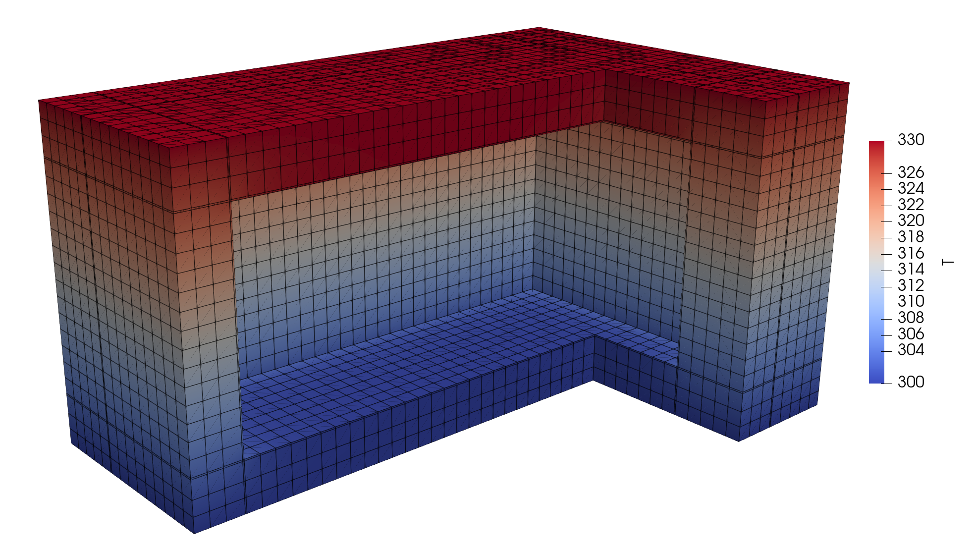
value = 330
[]
[bottom]
type = DirichletBC
variable = T
boundary = bottom
value = 300
[]
[]
[Executioner]
type = Steady # Steady state problem
solve_type = NEWTON # Perform a Newton solve
petsc_options_iname = '-pc_type -pc_hypre_type' # PETSc option pairs with values below
petsc_options_value = 'hypre boomeramg'
[]
[Outputs]
exodus = true # Output Exodus format
[]
Step 1: Run
An executable is available from loading the MOOSE conda or HPC module.
cd ~/projects/moose/tutorials/shield_multiphysics/inputs/step01_diffusion
moose-opt -i mesh.i --mesh-only
moose-opt -i step1.i
The simulation header gives a lot of helpful information
Framework Information:
MOOSE Version:           git commit 77c5910099 on 2025-05-28
LibMesh Version:
PETSc Version:           3.23.0
SLEPc Version:           3.23.0
Current Time:            Wed Jun  4 22:26:52 2025
Executable Timestamp:    Mon Jun  2 08:29:52 2025

Input File(s):
  /Users/giudgl/projects/moose_v9/tutorials/shield_multiphysics/inputs/step01_diffusion/step1.i

Checkpoint:
  Wall Time Interval:      Every 3600 s
  User Checkpoint:         Disabled
  # Checkpoints Kept:      2
  Execute On:              TIMESTEP_END

Parallelism:
  Num Processors:          1
  Num Threads:             1

Mesh:
  Parallel Type:           replicated
  Mesh Dimension:          3
  Spatial Dimension:       3
  Nodes:                   21692
  Elems:                   17920
  Num Subdomains:          4

Nonlinear System:
  Num DOFs:                21692
  Num Local DOFs:          21692
  Variables:               "T"
  Finite Element Types:    "LAGRANGE"
  Approximation Orders:    "FIRST"

Execution Information:
  Executioner:             Steady
  Solver Mode:             NEWTON
  PETSc Preconditioner:    hypre boomeramg strong_threshold: 0.7 (auto)
  MOOSE Preconditioner:    SMP (auto)
 0 Nonlinear |R| = 3.409028e+03
      0 Linear |R| = 3.409028e+03
      1 Linear |R| = 1.290229e+02
      2 Linear |R| = 1.113660e+01
      3 Linear |R| = 8.340899e-01
      4 Linear |R| = 5.736450e-02
      5 Linear |R| = 2.859743e-03
 1 Nonlinear |R| = 2.859743e-03
      0 Linear |R| = 2.859743e-03
      1 Linear |R| = 2.670323e-04
      2 Linear |R| = 1.878905e-05
      3 Linear |R| = 9.979916e-07
      4 Linear |R| = 7.651689e-08
      5 Linear |R| = 4.971569e-09
 2 Nonlinear |R| = 4.971578e-09
 Solve Converged!
Step 1: Result
Finite Element Method (FEM)
Function Approximation
To introduce the concept of FEM, consider a polynomial regression exercise. We can search for a polynomial function that solves the following problems:
Discrete example: Given sampled locations with associated values, we want our polynomial function to be as close to the input data as possible.
Continuous example: Given a complicated function, we want to have our polynomial function as close to the input function as possible.
Let us write the polynomial in the following form:
where are scalar coefficients (expansion coefficients) and monomials are "basis functions". Thus, the problem is to find such that is closest the the given points or a given function.
Polynomial Example (Discrete)
Define a set of points (Let's pick the points using ):
Substitute data into the polynomial model:
This results 4 equations for 3 unknowns () that can be expressed as the following linear system:
We want to get the function closest to the points. Distance in this case can be expressed by the discrete norm:
We want to minimize the norm of the squared distances ("least squares"):
which requires the solution of this problem:
which results in:
These coefficients define the solution function:
Polynomial Example (Continuous)
We want to minimize the squared distance between the known function () and the polynomial approximate () on a given domain :
The cumulative squared distance can be expressed as:
which we would like to minimize in a least-squares sense, with respect to the coefficients in (entries of ):
We can move the derivative with respect to into the integral:
which results in the following system (dropping the factor 2):
with
solving this sytem results in:
These coefficients define the solution function:
The coefficients are meaningless, they are just numbers used to define a function.
The solution is not the coefficients, but rather the function created when they are multiplied by their respective basis functions and summed.
The function is defined everywhere in the domain.
can be evaluated at the point , for example, by computing:
where the correspond to the coefficients in the solution vector, and the are the respective functions.
FEM can be used to solve both linear and nonlinear PDEs
FEM is a method for numerically approximating the solution to partial differential equations (PDEs). FEM is widely applicable for a large range of PDEs and domains.
Example PDEs: Have you seen them before? Are they linear/nonlinear? Coupled?
(1)(2)(3)FEM is a general method to discretize these equations
FEM finds a solution function that is made up of "shape functions" multiplied by coefficients and added together, just like in polynomial regression, except the functions are not typically as simple (although they can be).
The Galerkin Finite Element method is different from finite difference and finite volume methods because it finds a piecewise continuous function which is an approximate solution to the governing PDEs.
FEM provides an approximate solution. The true solution can only be represented as well as the shape function basis can represent it!
FEM is supported by a rich mathematical theory with proofs about accuracy, stability, convergence and solution uniqueness.
Weak Form
Using FEM to find the solution to a PDE starts with forming a "weighted residual" or "variational statement" or "weak form", this processes if referred to here as generating a weak form.
The weak form provides flexibility, both mathematically and numerically and it is needed by MOOSE to solve a problem.
Generating a weak form generally involves these steps:
Write down strong form of PDE.
Rearrange terms so that zero is on the right of the equals sign.
Multiply the whole equation by a "test" function .
Integrate the whole equation over the domain .
Integrate by parts and use the divergence theorem to get the desired derivative order on your functions and simultaneously generate boundary integrals.
Obtain the weak form for the equations listed on the previous slide and the shape functions.
Looking back
Polynomial fitting:
Form equations that the coefficients of a polynomial function must satisfy to fit
Solve the linear system
Reconstruct the fit by evaluating the polynomial defined by its coefficients
Finite Element method:
Form equations on each element to minimize the residual of an equation
Solve the linear system
Reconstruct the function
Re-evaluate the equation and iterate (for nonlinear equations)
Integration by Parts and Divergence Theorem
Suppose is a scalar function, is a vector function, and both are continuously differentiable functions, then the product rule states:
The function can be integrated over the volume and rearranged as:
(4)The divergence theorem transforms a volume integral into a surface integral on surface :
(5)where is the outward normal vector for surface . Combining Eq. (4) and Eq. (5) yield:
(6)Example: Advection-Diffusion
(1) Write the strong form of the equation:
(2) Rearrange to get zero on the right-hand side:
(3) Multiply by the test function :
(4) Integrate over the domain :
(5) Integrate by parts and apply the divergence theorem, by using Eq. (6) on the left-most term of the PDE:
Write in inner product notation. Each term of the equation will inherit from an existing MOOSE type as shown below.
(7)Corresponding MOOSE input file blocks
[Kernels]
  [diffusion]
    type = CoefDiffusion
    variable = 'u'
    coef = ${k}
  []
[]
[BCs]
  [inlet_flux]
    type = FunctionNeumannBC
    variable = 'u'
    boundary = 'left'
    function = box_flux
  []
  [outlet_avective_flux]
    type = ConservativeAdvectionBC
    variable = 'u'
    boundary = 'right'
    velocity_function = 'beta'
  []
  [outlet_diffusive_flux]
    type = DiffusionFluxBC
    variable = 'u'
    boundary = 'right'
  []
  # walls are 0 flux (achieved with no BC, this depends on the kernels used)
[]
[Kernels]
  [advection]
    type = ConservativeAdvection
    variable = u
    velocity = ${beta}
  []
[]
[Kernels]
  [force]
    type = BodyForce
    variable = u
    function = f_fn
  []
[]
Finite Element Shape Functions
Basis Functions
While the weak form is essentially what is needed for adding physics to MOOSE, in traditional finite element software more work is necessary.
The weak form must be discretized using a set of "basis functions" amenable for manipulation by a computer.

Images copyright Becker et al. (1981)

Shape Functions
The discretized expansion of takes on the following form:
where are the "basis functions", which form the basis for the "trial function", . is the total number of functions for the discretized domain.
The gradient of can be expanded similarly:
In the Galerkin finite element method, the same basis functions are used for both the trial and test functions:
Substituting these expansions back into the example weak form (Eq. (7)) yields:
(8)The left-hand side of the equation above is referred to as the component of the "residual vector," .
Shape Functions are the functions that get multiplied by coefficients and summed to form the solution.
Individual shape functions are restrictions of the global basis functions to individual elements.
They are analogous to the functions from polynomial fitting (in fact, you can use those as shape functions).
Typical shape function families: Lagrange, Hermite, Hierarchic, Monomial, Clough-Tocher
Lagrange shape functions are the most common, which are interpolatory at the nodes, i.e., the coefficients correspond to the values of the functions at the nodes.
Example 1D Shape Functions


2D Lagrange Shape Functions
Example bi-quadratic basis functions defined on the (square) Quad9 element:
(left) is associated to a "corner" node, it is zero on the opposite edges.
(middle) is associated to a "mid-edge" node, it is zero on all other edges.
(right) is associated to the "center" node, it is symmetric and on the element.


Setting Shape Functions in a MOOSE input file
Shape functions can be set for each variable in the Variables block:
[Variables]
  [u]
    order = FIRST
    family = LAGRANGE
    block = 0
  []
  [v]
    order = FIRST
    family = LAGRANGE
    block = 1
  []
[]
Numerical Implementation
Numerical Integration
The only remaining non-discretized parts of the weak form are the integrals. First, split the domain integral into a sum of integrals over elements:
(9)Through a change of variables, the element integrals are mapped to integrals over the "reference" elements .
where is the Jacobian of the map from the physical element to the reference element.
Reference Element (Quad9)

Quadrature
Quadrature, typically "Gaussian quadrature", is used to approximate the reference element integrals numerically.
where is the weight function at quadrature point .
Under certain common situations, the quadrature approximation is exact. For example, in 1 dimension, Gaussian Quadrature can exactly integrate polynomials of order with quadrature points.
Applying the quadrature to Eq. (9) we can simply compute:
where is the spatial location of the quadrature point and is its associated weight.
MOOSE handles multiplication by the Jacobian () and the weight () automatically, thus your Kernel object is only responsible for computing the part of the integrand.
Sampling at the quadrature points yields:
Thus, the weak form of Eq. (8) becomes:
(10)The second sum is over boundary faces, . MOOSE Kernel or BoundaryCondition objects provide each of the terms in square brackets (evaluated at or as necessary), respectively.
Intermediate summary
There is a mesh, with cells and functions, polynomials, defined by their coefficients
We plug in these functions in the PDEs, then obtain a weak form
We evaluate the integrals in the weak form using a quadrature, thus forming a set of equations
Now let's solve these equations to obtain the coefficients
Newton's Method
Newton's method is a "root finding" method with good convergence properties, in "update form", for finding roots of a scalar equation it is defined as: , is given by

Newton's Method in MOOSE
The residual, , as defined by Eq. (10) is a nonlinear system of equations,
that is used to solve for the coefficients .
For this system of nonlinear equations Newton's method is defined as:
(11)where is the Jacobian matrix evaluated at the current iterate:
MOOSE Solve Types
The solve type is specified in the [Executioner] block within the input file:
[Executioner]
  solve_type = PJFNK
Available options include:
PJFNK: Preconditioned Jacobian Free Newton Krylov (default)
JFNK: Jacobian Free Newton Krylov
NEWTON: Performs solve using exact Jacobian for preconditioning
FD: PETSc computes terms using a finite difference method (debug)
JFNK
Uses a Krylov subspace-based linear solver
(12)The action of the Jacobian is approximated by:
(13)The Kernel method computeQpResidual is called to compute during the nonlinear step (Eq. (11)).
During each linear step of JFNK, the computeQpResidual method is called to approximate the action of the Jacobian on the Krylov vector.
PJFNK
The action of the preconditioned Jacobian is approximated by:
(14)The Kernel method computeQpResidual is called to compute during the nonlinear step (Eq. (11)).
During each linear step of PJFNK, the computeQpResidual method is called to approximate the action of the Jacobian on the Krylov vector. The computeQpJacobian and computeQpOffDiagJacobian methods are used to compute values for the preconditioning matrix.
NEWTON
The Kernel method computeQpResidual is called to compute during the nonlinear step (Eq. (11)).
The computeQpJacobian and computeQpOffDiagJacobian methods are used to compute the preconditioning matrix. It is assumed that the preconditioning matrix is the Jacobian matrix, thus the residual and Jacobian calculations are able to remain constant during linear iterations.
Preconditioning
Select a preconditioner using PETSC options, either in the executioner or in the [Preconditioning] block:
[Executioner]
  type = Steady
  petsc_options_iname = '-pc_type -pc_hypre_type'
  petsc_options_value = 'hypre boomeramg'
Some examples:
LU : form the actual Jacobian inverse, useful for small to medium problems but does not scale well
Hypre BoomerAMG : algebraic multi-grid, works well for diffusive problems
Jacobi : preconditions with the diagonal, row sum, or row max of Jacobian
For parallel preconditioners, the sub-block (on-process) preconditioners can be controlled with the PETSc option -sub_pc_type. E.g. for a parallel block Jacobi preconditioner (-pc_type bjacobi) the sub-block preconditioner could be set to ILU or LU etc. with -sub_pc_type ilu, -sub_pc_type lu, etc.
Summary
The Finite Element Method is a way of numerically approximating the solution of PDEs.
Just like polynomial fitting, FEM finds coefficients for basis functions.
The solution is the combination of the coefficients and the basis functions, and the solution can be sampled anywhere in the domain.
Integrals are computed numerically using quadrature.
Newton's method provides a mechanism for solving a system of nonlinear equations.
The Preconditioned Jacobian Free Newton Krylov (PJFNK) method allows us to avoid explicitly forming the Jacobian matrix while still computing its action.
Automatic Jacobian Calculation
MOOSE uses forward mode automatic differentiation from the MetaPhysicL package.
Moving forward, the idea is for application developers to be able to develop entire apps without writing a single Jacobian statement. This has the potential to decrease application development time.
In terms of computing performance, presently AD Jacobians are slower to compute than hand-coded Jacobians, but they parallelize extremely well and can benefit from using a NEWTON solve, which often results in decreased solve time overall.
Relies on two techniques:
chain rule
operator overloading
One thing to note is that the derivatives are with regards to the degrees of freedom, but the residual is computed at quadrature points! There are therefore often several non-zero coefficients even for simply (value of variable u at a quadrature point).
Manual Jacobian Calculation
The remainder of the tutorial will focus on using automatic differentiation (AD) for computing Jacobian terms, but it is possible to compute them manually.
It is recommended that all new Kernel objects use AD.
FEM Derivative Identities
The following relationships are useful when computing Jacobian terms.
(15)(16)Newton for a Simple Equation
Again, consider the advection-diffusion equation with nonlinear , , and :
Thus, the component of the residual vector is:
Using the previously-defined rules in Eq. (15) and Eq. (16) for and , the entry of the Jacobian is then:
That even for this "simple" equation, the Jacobian entries are nontrivial: they depend on the partial derivatives of , , and , which may be difficult or time-consuming to compute analytically.
In a multiphysics setting with many coupled equations and complicated material properties, the Jacobian might be extremely difficult to determine.
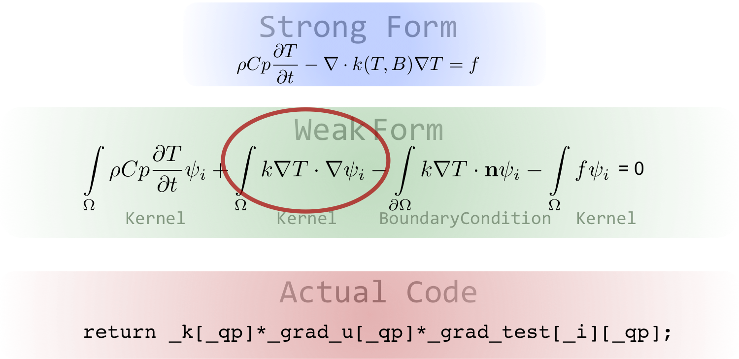
Step 2: Simple Heat Conduction Kernel
Implementing equations in MOOSE
To implement the Heat Conduction equation, we will use a Kernel object to compute the residual and the Jacobian of the diffusion term:
where is the thermal diffusivity.
A Kernel is C++ class, which inherits from MooseObject that is used by MOOSE for coding volume integrals of a partial differential equation (PDE).
Kernel System
A system for computing the residual contribution from a volumetric term within a PDE using the Galerkin finite element method.
Kernel Object
A Kernel objects represents one or more terms in a PDE.
A Kernel object computes the residual at each quadrature point on every element. When forming a Jacobian, the Kernel object is also called to compute its components at each quadrature point.
Diffusion
Recall the steady-state diffusion equation on the 3D domain :
The weak form of this equation includes a volume integral, which in inner-product notation, is given by:
where are the test functions and is the finite element solution.
This integral is approximated by the kernel using the specified quadrature.
Input Parameters
Every object in MOOSE includes a set of custom parameters within an InputParameters object that is used to construct the object.
Required parameters
Some object parameters are required. MOOSE will error if they are not provided in the input file.
[Kernels]
  [diff]
    type = Diffusion
  []
[]
The example above will error because the variable parameter is missing.
The MOOSE VSCode plugin will automatically create a <required_parameter> = line for each required parameter when using the syntax auto-complete.
Optional Parameter(s) have a default
If the value of a parameter is standard, it does not need to be always included in the input file, unless the user wants to change its value! In the example below, the block parameter is not specified, which means the default (empty) is applied.
[Kernels]
  [diff]
    type = Diffusion
    variable = u
  []
[]
The MOOSE VSCode plugin will automatically create a <optional_parameter> = <default_value> line for an optional parameter when using the auto-complete feature and selecting said parameter.
Coupled Variable
Various types of objects in MOOSE can be coupled to variables. MOOSE will then automatically compute the local variable values when executing the object.
[Variables]
  [P][]
  [T][]
[]

[UserObjects]
  [temp_pressure_check]
    type = CheckTemperatureAndPressure
    temperature = T
    pressure = P # if not provided a value of 101.325 would be used
  []
[]
Within the input file it is possible to used a variable name or a constant value for a coupledVar parameter.
pressure = P
pressure = 42
Range Checked Parameters
Input constant values may be restricted to a range of values. This is enforced programmatically, and MOOSE will error if the user passes a value out of the specified bounds.
Documentation
Each application is capable of generating documentation from the validParams functions.
Option 1: Command line --dump
--dump [optional search string]the search string may contain wildcard characters
searches both block names and parameters
Option 2: Command line --show-input generates a tree based on your input file\\
Option 3: mooseframework.org/syntax
Supported types
MOOSE can support integer, float, vector, string, ... parameters. However this is specified in each object, and types cannot be changed in the input file.
Other supported parameter types include:
PointRealVectorValueRealTensorValueSubdomainIDstd::map<std::string, Real>
MOOSE uses a large number of string types to make InputParameters more context-aware. All of these types can be treated just like strings, but will cause compile errors if mixed improperly in the template functions.
SubdomainName
BoundaryName
FileName
DataFileName
VariableName
FunctionName
UserObjectName
PostprocessorName
MeshFileName
OutFileName
NonlinearVariableName
AuxVariableName
Enumerations
MOOSE supports enumerations as parameters. An enumeration is a fixed list of options, that the user may then select from. Defaults are supported for these enumerations.
In the example below, the value_type parameters can take max or min values, with a default of max. If you specify abc to value_type, it will error.
[Postprocessors]
  [max]
    type = ElementExtremeValue
    variable = u
  []
  [min]
    type = ElementExtremeValue
    variable = u
    value_type = min
  []
[]
Input file variables
Variables can be defined in the input file, and substituted anywhere below their definition.
diff = 3

[Variables]
  [u]
    family = LAGRANGE
    initial_condition = ${diff}
  []
[]
Input file parsed expressions for basic math
We can have the parser perform simple math for us using the ${fparser <some math>} syntax. The available syntax can be found on this page.
diff = 3
scale_diff = 2
offset_diff = 1

[Variables]
  [u]
    family = LAGRANGE
    initial_condition = ${fparse offset_diff + scale_diff * diff}  # = 1 + 2 * 3
  []
[]
Unit conversions in the input file
MOOSE supports both S.I. and imperial units. But everything must be consistent. Your input file, your mesh, and your material properties must use the same unit system. To help adapt your input file, we provide unit conversion capabilities.
length_in = 25
length_m = ${units 23 in -> m}

# we can still use input file variables too
length_meters = ${units ${length_in} in -> m}
A table of unit and units names is provided at this link.
Global parameters
Global parameters are defined in a special block and are substituted everywhere in the input they can be. This lets us reduce the size of the input file, at the cost these more implicit substitutions.
[GlobalParams]
  second_order = true # this will go in the [Mesh] block
  order = SECOND      # this will go in the each variable object
[]

[Variables]
  [u]
  # the order is being changed to SECOND without writing it down here
  []
  [v]
    # we don't want v to be second order
    order = FIRST
  []
[]
Be careful with global parameters with common parameter names such as block or variable. They will apply to every single object, even the ones you did not think of.
Combining input files using "!include"
Input files can be concatenated using the !include <other input file.i> syntax. This is helpful to:
share common input syntax between multiple inputs (for example a steady and a transient simulations, sharing the same mesh)
build long input files in multiple steps
Step 2: Heat Conduction Kernel
(continued)
CoefDiffusion Kernel
The heat conduction equation amounts to a diffusion equation with a coefficient.
where is the thermal diffusivity.
To implement the coefficient a new Kernel object must be used: CoefDiffusion.
This object inherits from Diffusion and will use input parameters for specifying the diffusivity.
Step 2: Input File
We introduce block restriction to differentiate between water and concrete. Block restriction is a common feature of MOOSE objects, introduced by setting
block = 'concrete'
In this example, we limit the heat conduction equation to the concrete and aluminum blocks.
[Kernels]
  [diffusion_water]
    type = CoefDiffusion
    variable = T
    coef = 0.6
    block = water
  []
  [diffusion_concrete_hd]
    type = CoefDiffusion
    variable = T
    coef = 5
    block = concrete_hd
  []
  [diffusion_concrete]
    type = CoefDiffusion
    variable = T
    coef = 2.25
    block = concrete
  []
  [diffusion_Al]
    type = CoefDiffusion
    variable = T
    coef = 175
    block = Al
  []
[]
Step 2: Run
cd ~/projects/moose/tutorials/shield_multiphysics/inputs/step02_coef_diffusion
moose-opt -i step2.i
Step 2: Result
Output System
A system for outputting simulation data to the screen or files.
The output system is designed to be just like any other system in MOOSE: modular and expandable.
It is possible to create multiple output objects for outputting:
at specific time or timestep intervals,
custom subsets of variables, and
to various file types.
There exists a short-cut syntax for common output types as well as common parameters.
Short-cut Syntax
The following two methods for creating an Output object are equivalent within the internals of MOOSE.
[Outputs]
  exodus = true
[]
[Outputs]
  [out]
    type = Exodus
  []
[]
Customizing Output
The content of each Output can customized, see for example for an Exodus output:
[Outputs]
  [out]
    type = Exodus
    output_material_properties = true
    # removes some quantities from the output
    hide = 'power_pp pressure_var'
  []
[]
Common Parameters
[Outputs]
  interval = 10 # this is a time step interval
  [exo]
    type = Exodus
    interval = 1 # overrides interval from top-level
  []
  [cp]
    type = Checkpoint # Uses interval specified from top-level
  []
[]
Output Names
The default naming scheme for output files utilizes the input file name (e.g., input.i) with a suffix that differs depending on how the output is defined: An "_out" suffix is used for Outputs created using the short-cut syntax. sub-blocks use the actual sub-block name as the suffix.
[Outputs]
  exodus = true    # creates input_out.e
  [other]          # creates input_other.e
     type = Exodus
     interval = 2
  []
  [base]
    type = Exodus
    file_base = out # creates out.e
  []
[]
| Short-cut | Sub-block ("type=") | Description |
|---|---|---|
| console | Console | Writes to the screen and optionally a file |
| exodus | Exodus | The most common,well supported, and controllable output type |
| vtk | VTK | Visualization Toolkit format, requires --enable-vtk when building libMesh |
| gmv | GMV | General Mesh Viewer format |
| nemesis | Nemesis | Parallel ExodusII format |
| tecplot | Tecplot | Requires --enable-tecplot when building libMesh |
| xda | XDA | libMesh internal format (ascii) |
| xdr | XDR | libMesh internal format (binary) |
| csv | CSV | Comma separated scalar values |
| gnuplot | GNUPlot | Only support scalar outputs |
| checkpoint | Checkpoint | MOOSE internal format used for restart and recovery |
Paraview can read many of these (CSV, Exodus, Nemesis, VTK, GMV)
Step 3: Boundary conditions
Fixed temperatures at the boundary conditions are simple but not realistic. We want to have:
a fixed heat flux from the micro-reactor inside the concrete cavity
natural convection boundary conditions with the air around the shield
convective boundary conditions with the water block
Boundary Condition System
System for computing residual contributions from boundary terms of a PDE.
A BoundaryCondition (BC) object computes a residual on a boundary (or internal side) of a domain.
There are two flavors of BC objects: Nodal and Integrated.
Integrated BC
Integrated BCs are integrated over a boundary or internal side. They are meant to add a surface integral term, coming from example from the application of the divergence theorem.
This integral is computed using a surface quadrature.
Non-Integrated BC
Non-integrated BCs set values of the residual directly on a boundary or internal side. They do not rely a quadrature-point based integration.
Dirichlet BCs
Set a condition on the value of a variable on a boundary:
becomes
Integrated BCs
Integrated BCs (including Neumann BCs) are actually integrated over the external face of an element.
becomes:
If , then the boundary integral is zero ("natural boundary condition").
Periodic BCs
Periodic boundary conditions are useful for modeling quasi-infinite domains and systems with conserved quantities.
1D, 2D, and 3D
With mesh adaptivity
Can be restricted to specific variables
Supports arbitrary translation vectors for defining periodicity
Function System
A system for defining analytic expressions based on the spatial location (, , ) and time, .
A Function can depend an other functions, but not on material properties or variables.
Function Use
Many objects exist in MOOSE that utilize a function, such as:
FunctionDirichletBCFunctionNeumannBCFunctionICBodyForce
Each of these objects has a "function" parameter which is set in the input file, and controls which Function object is used.
Parsed Function
A ParsedFunction allow functions to be defined by strings directly in the input file, e.g.:
[Functions]
  [sin_fn]
    type = ParsedFunction
    expression = sin(x)
  []
  [cos_fn]
    type = ParsedFunction
    expression = cos(x)
  []
  [fn]
    type = ParsedFunction
    # Inputs we will use in the parsed expression
    symbol_values = 'sin_fn cos_fn'
    # Short names for each input
    symbol_names = 's c'
    # Expression to parse
    expression = 's/c'
  []
[]
It is possible to include other functions, as shown above, as well as scalar variables and postprocessor values with the function definition.
Default Functions
Whenever an object uses a Function-name parameter, the user may elect to instead write the expression of a x,y,z,t function directly in that parameter. A ParsedFunction will automatically be created for this function.
A ParsedFunction or ConstantFunction object is automatically constructed based on the default value if a function name is not supplied in the input file.
Using a Function in our model
Let's vary the water temperature in time
  [water_convection]
    type = ADConvectiveHeatFluxBC
    variable = T
    boundary = 'water_boundary_inwards'
    T_infinity = 300.0
    heat_transfer_coefficient = 30
  []
The same BC object can accept a function parameter:
  [water_convection]
    type = ADConvectiveHeatFluxBC
    variable = T
    boundary = 'water_boundary_inwards'
    T_infinity_functor = water_T_ramp
    heat_transfer_coefficient = 30
  []

[Functions]
  [water_T_ramp]
    type = PiecewiseLinear
    x = '0 10 100'
    y = '300 290 290'
  []
[]
Let's vary the power input in space
  [from_reactor]
    type = NeumannBC
    variable = T
    boundary = inner_cavity
    # 100 kW reactor, 108 m2 cavity area
    value = '${fparse 1e5 / 108}'
  []
This time we have to select a different object:
  [from_reactor]
    type = FunctionNeumannBC
    variable = T
    boundary = inner_cavity
    # 100 kW reactor, 108 m2 cavity area
    function = 'heat_flux'
  []

[Functions]
  [heat_flux]
    type = ParsedFunction
    # apply heat flux only above z=1m
    expression = 'if(z > 1, 1e5 / 108, 0)'
  []
[]
Step 3: Boundary conditions
(continued)
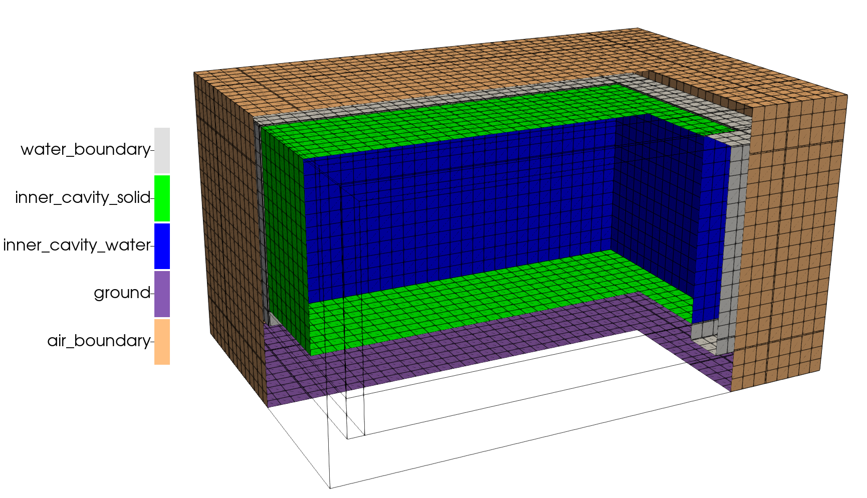
First, the sidesets must be added / present in the mesh. We modified the meshing script to generate sidesets for our boundary conditions
!include ../step01_diffusion/mesh.i

[Mesh]
  [add_concrete_outer_boundary]
    type = RenameBoundaryGenerator
    input = rename_boundaries_step3
    old_boundary = 'left         right        front        bottom top          back'
    new_boundary = 'air_boundary air_boundary air_boundary ground air_boundary air_boundary'
  []
  [add_water_concrete_interface]
    type = SideSetsBetweenSubdomainsGenerator
    input = add_concrete_outer_boundary
    primary_block = 'water water water'
    paired_block = 'concrete_hd concrete Al'
    new_boundary = 'water_boundary'
  []
  [add_water_concrete_interface_inwards]
    type = SideSetsBetweenSubdomainsGenerator
    input = add_water_concrete_interface
    primary_block = 'concrete_hd concrete Al'
    paired_block = 'water water water'
    new_boundary = 'water_boundary_inwards'
  []
  [add_inner_cavity_solid]
    type = SideSetsAroundSubdomainGenerator
    input = add_water_concrete_interface_inwards
    block = Al
    new_boundary = 'inner_cavity_solid'
    include_only_external_sides = true
  []
  [add_inner_cavity_water]
    type = SideSetsAroundSubdomainGenerator
    input = add_inner_cavity_solid
    block = water
    new_boundary = 'inner_cavity_water'
    include_only_external_sides = true
  []
[]
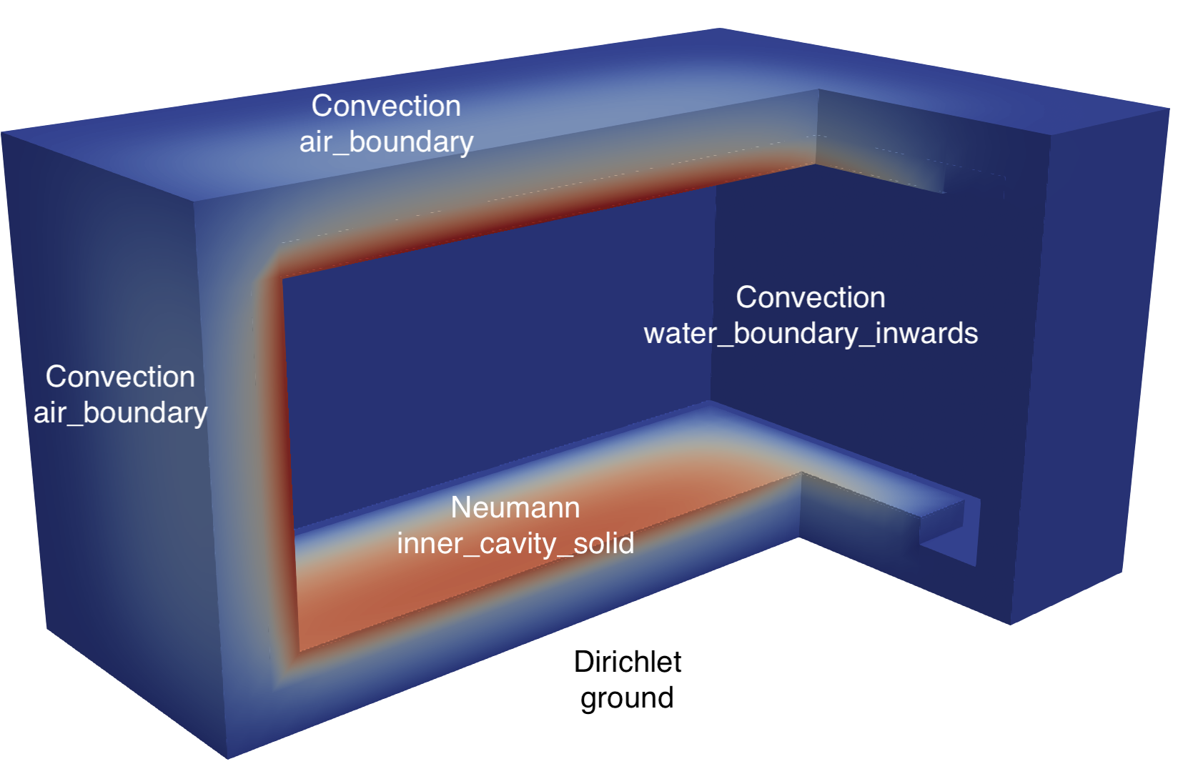
We apply a NeumannBC for fixed heat flux on the inner cavity.
[BCs]
  [from_reactor]
    type = NeumannBC
    variable = T
    boundary = inner_cavity_solid
    # 5 MW reactor, only 50kW removed through radiation, 144 m2 cavity area
    value = '${fparse 5e4 / 144}'
  []
[]
We apply a DirichletBC for a fixed temperature with the ground.
[BCs]
  [ground]
    type = DirichletBC
    variable = T
    value = 300
    boundary = 'ground'
  []
[]
Convection with air using ConvectiveHeatFluxBC.
[BCs]
  [air_convection]
    type = ConvectiveHeatFluxBC
    variable = T
    boundary = 'air_boundary'
    T_infinity = 300.0
    # The heat transfer coefficient should be obtained from a correlation
    heat_transfer_coefficient = 10
  []
[]
Note that sidesets are oriented. The variables on which the BC is applied must be defined on the primary side (opposite the normal) of the sideset. For an external boundary, this is never a concern.
Convection with water
We use the same boundary condition for the water boundary as for the convection with air for now. When we introduce a separate variable for the water temperature, we will revisit this. We use the 'water_boundary_inwards' surface because the solid block is on its primary side.
[BCs]
  [water_convection]
    type = ConvectiveHeatFluxBC
    variable = T
    boundary = 'water_boundary_inwards'
    T_infinity = 300.0
    # The heat transfer coefficient should be obtained from a correlation
    heat_transfer_coefficient = 600
  []
[]
Summary of the boundary conditions:
Step 3: Input File
[Mesh]
  [fmg]
    type = FileMeshGenerator
    file = 'mesh_in.e'
  []
[]

[Variables]
  [T]
    # Adds a Linear Lagrange variable by default
    block = 'concrete concrete_hd Al'
  []
[]

[Kernels]
  [diffusion_concrete_hd]
    type = CoefDiffusion
    variable = T
    coef = 5
    block = concrete_hd
  []
  [diffusion_concrete]
    type = CoefDiffusion
    variable = T
    coef = 2.25
    block = concrete
  []
  [diffusion_Al]
    type = CoefDiffusion
    variable = T
    coef = 175
    block = Al
  []
[]

[BCs]
  [from_reactor]
    type = NeumannBC
    variable = T
    boundary = inner_cavity_solid
    # 5 MW reactor, only 50kW removed through radiation, 144 m2 cavity area
    value = '${fparse 5e4 / 144}'
  []
  [air_convection]
    type = ConvectiveHeatFluxBC
    variable = T
    boundary = 'air_boundary'
    T_infinity = 300.0
    # The heat transfer coefficient should be obtained from a correlation
    heat_transfer_coefficient = 10
  []
  [ground]
    type = DirichletBC
    variable = T
    value = 300
    boundary = 'ground'
  []
  [water_convection]
    type = ConvectiveHeatFluxBC
    variable = T
    boundary = 'water_boundary_inwards'
    T_infinity = 300.0
    # The heat transfer coefficient should be obtained from a correlation
    heat_transfer_coefficient = 600
  []
[]

[Problem]
  # No kernels on the water domain
  kernel_coverage_check = false
[]

[Executioner]
  type = Steady # Steady state problem
  solve_type = NEWTON # Perform a Newton solve
  petsc_options_iname = '-pc_type -pc_hypre_type' # PETSc option pairs with values below
  petsc_options_value = 'hypre boomeramg'
[]

[Outputs]
  exodus = true # Output Exodus format
[]
Step 3: Run
cd ~/projects/moose/tutorials/shield_multiphysics/inputs/step03_boundary_conditions
moose-opt -i mesh.i --mesh-only
moose-opt -i step3.i
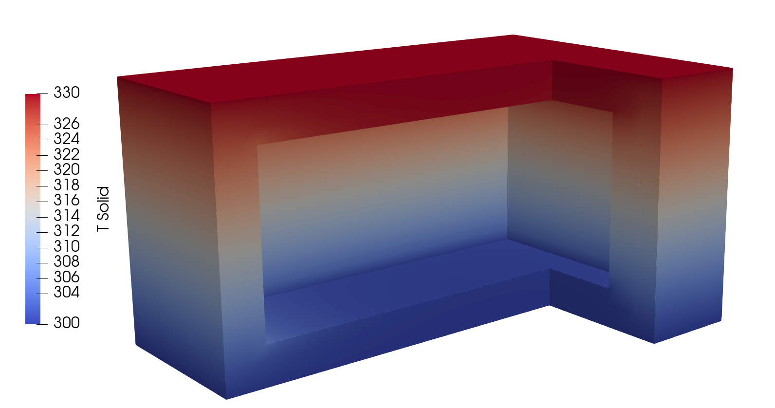
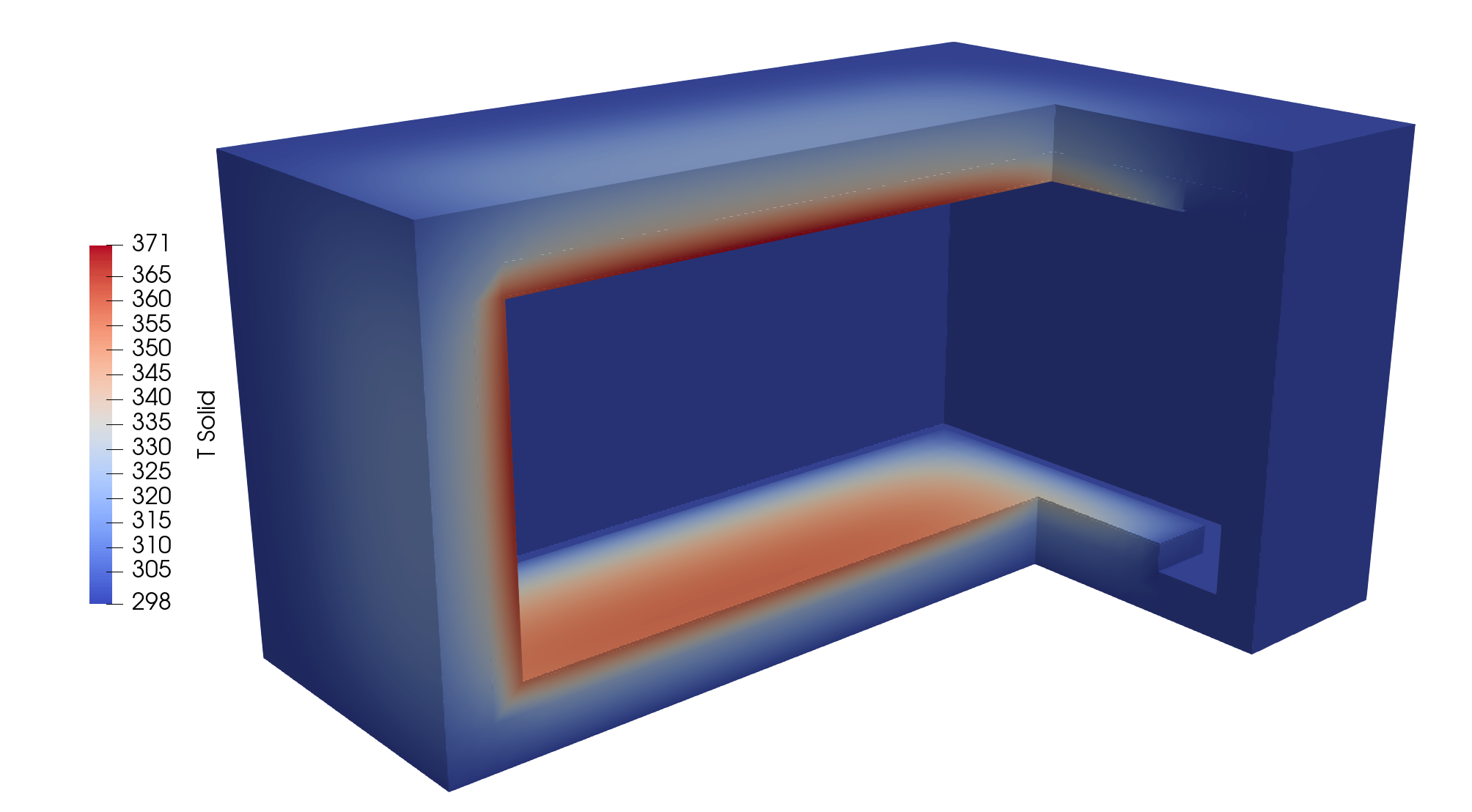
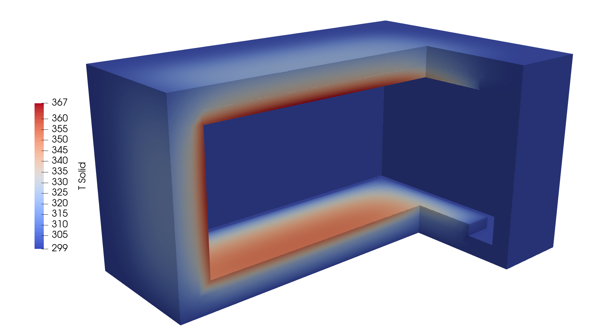
Step 3: Result
We only show the solid temperature. The water temperature is a constant for now.
Step 4: Heat Conduction kernel with Material
Instead of passing constant coefficients to the heat conduction kernel, we use the Material system to supply the values.
where is the thermal conductivity.
This system allows for properties that vary in space and time, that can be coupled to variables in the simulation.
Material System
A system for defining material properties to be used by multiple systems and allow for variable coupling.
The material system operates by creating a producer/consumer relationship among objects
Materialobjects produce properties.Other MOOSE objects (including materials) consume these properties.
Material Property Evaluation
Quantities are recomputed at quadrature points, as needed.
Multiple Material objects may define the same "property" for different parts of the subdomain or boundaries.
Stateful Material Properties
Values of material properties can be stored at the previous ("old") and two-before ("older") time steps.
It can be useful to have "old" values of Material properties available in a simulation, such as in solid mechanics plasticity constitutive models.
Traditionally, this type of value is called a "state variable"; in MOOSE, they are called "stateful material properties".
Stateful Material properties require more memory.
Default Material Properties
Material properties may have default values, which can be found in the documentation, and are automatically prefilled when using the syntax auto-complete.
Only scalar (Real) valued properties may have defaults.
Material Property Output
Output of Material properties is enabled by setting the "outputs" parameter.
The following example creates two additional variables called "mat1" and "mat2" that will show up in the output file.
[Materials]
  [block_1]
    type = OutputTestMaterial
    block = 1
    output_properties = 'real_property tensor_property'
    outputs = exodus
    variable = u
  []
  [block_2]
    type = OutputTestMaterial
    block = 2
    output_properties = 'vector_property tensor_property'
    outputs = exodus
    variable = u
  []
[]

[Outputs]
  exodus = true
[]
Supported Property Types for Output
Material properties can be of arbitrary (C++) type, but not all types can be output.
| Type | AuxKernel | Variable Name(s) |
|---|---|---|
| Real | MaterialRealAux | prop |
| RealVectorValue | MaterialRealVectorValueAux | prop_1, prop_2, and prop_3 |
| RealStdVector | MaterialStdVectorAux | prop_1, prop_2, and prop_3 |
| RealTensorValue | MaterialRealTensorValueAux | prop_11, prop_12, prop_13, prop_21, etc. |
| DenseMatrix | MaterialRealDenseMatrixAux | prop_11, prop_12, prop_13, prop_21, etc. |
AD-material property types can also be output.
Step 4: Heat Conduction with Material
(continued)
HeatConductionMaterial
Three material properties must be produced for consumption by kernels of the heat conduction equation:
thermal conductivity by the conduction term
density and specific heat by the time derivative of the energy
Both shall be computed with a single Material object: HeatConductionMaterial.
[Materials]
  [concrete_hd]
    type = ADHeatConductionMaterial
    block = concrete_hd
    temp = 'T'
    # we specify a function of time, temperature is passed as the time argument
    # in the material
    thermal_conductivity_temperature_function = '5.0 + 0.001 * t'
  []
  [concrete]
    type = ADHeatConductionMaterial
    block = concrete
    temp = 'T'
    thermal_conductivity_temperature_function = '2.25 + 0.001 * t'
  []
  [Al]
    type = ADHeatConductionMaterial
    block = Al
    temp = T
    thermal_conductivity_temperature_function = '175'
  []
[]
HeatConduction Kernel
The CoefDiffusion Kernel object uses input parameters for defining the thermal conductivity. Instead, the HeatConduction Kernel utilizes the material properties defined in HeatConductionMaterial automatically.
[Kernels]
  [diffusion_concrete]
    type = ADHeatConduction
    variable = T
  []
[]
Note: we use kernels with automatic differentiation (AD) for simplicity.
Step 4: Input File
[Mesh]
  [fmg]
    type = FileMeshGenerator
    file = '../step03_boundary_conditions/mesh_in.e'
  []
[]

[Variables]
  [T]
    # Adds a Linear Lagrange variable by default
    block = 'concrete_hd concrete Al'
  []
[]

[Kernels]
  [diffusion_concrete]
    type = ADHeatConduction
    variable = T
  []
[]

[Materials]
  [concrete_hd]
    type = ADHeatConductionMaterial
    block = concrete_hd
    temp = 'T'
    # we specify a function of time, temperature is passed as the time argument
    # in the material
    thermal_conductivity_temperature_function = '5.0 + 0.001 * t'
  []
  [concrete]
    type = ADHeatConductionMaterial
    block = concrete
    temp = 'T'
    thermal_conductivity_temperature_function = '2.25 + 0.001 * t'
  []
  [Al]
    type = ADHeatConductionMaterial
    block = Al
    temp = T
    thermal_conductivity_temperature_function = '175'
  []
[]

[BCs]
  [from_reactor]
    type = NeumannBC
    variable = T
    boundary = inner_cavity_solid
    # 5 MW reactor, only 50 kW removed from radiation, 144 m2 cavity area
    value = '${fparse 5e4 / 144}'
  []
  [air_convection]
    type = ADConvectiveHeatFluxBC
    variable = T
    boundary = 'air_boundary'
    T_infinity = 300.0
    # The heat transfer coefficient should be obtained from a correlation
    heat_transfer_coefficient = 10
  []
  [ground]
    type = DirichletBC
    variable = T
    value = 300
    boundary = 'ground'
  []
  [water_convection]
    type = ADConvectiveHeatFluxBC
    variable = T
    boundary = 'water_boundary_inwards'
    T_infinity = 300.0
    # The heat transfer coefficient should be obtained from a correlation
    heat_transfer_coefficient = 600
  []
[]

[Problem]
  # No kernels on the water domain
  kernel_coverage_check = false
  # No materials on the water domain
  material_coverage_check = false
[]

[Executioner]
  type = Steady # Steady state problem
  solve_type = NEWTON # Perform a Newton solve, uses AD to compute Jacobian terms
  petsc_options_iname = '-pc_type -pc_hypre_type' # PETSc option pairs with values below
  petsc_options_value = 'hypre boomeramg'
[]

[Outputs]
  exodus = true # Output Exodus format
[]
Step 4: Run
cd ~/projects/moose/tutorials/shield_multiphysics/inputs/step04_heat_conduction
moose-opt -i step4.i
Step 4: Result
Step 5: Auxiliary Variables
Auxiliary System
A system for direct calculation of field variables ("AuxVariables") that is designed for postprocessing, coupling, and proxy calculations.
The term "nonlinear variable" is defined, in MOOSE language, as a variable that is being solved for using a nonlinear system of PDEs using Kernel and BoundaryCondition objects.
The term "auxiliary variable" is defined, in MOOSE language, as a variable that is directly calculated using an AuxKernel object.
AuxVariables
Auxiliary variables are declared in the [AuxVariables] input file block
Auxiliary variables are field variables that are associated with finite element shape functions and can serve as a proxy for nonlinear variables
Auxiliary variables currently come in two flavors:
Element (e.g. constant or higher order monomials)
Nodal (e.g. linear Lagrange)
Auxiliary variables have "old" and "older" states, from previous time steps, just like nonlinear variables
Elemental Auxiliary Variables
Element auxiliary variables can compute:
average values per element, if stored in a constant monomial variable
spatial profiles using higher order variables
AuxKernel objects computing elemental values can couple to nonlinear variables and both element and nodal auxiliary variables
[AuxVariables]
  [aux]
    order = CONSTANT
    family = MONOMIAL
  []
[]
Nodal Auxiliary Variables
Element auxiliary variables are computed at each node and are stored as linear Lagrange variables
AuxKernel objects computing nodal values can only couple to nodal nonlinear variables and other nodal auxiliary variables
[AuxVariables]
  [aux]
    order = LAGRANGE
    family = FIRST
  []
[]
VectorAuxKernel Objects
VectorAuxKernels can compute vector auxiliary variables.
The auxiliary variable will have to be one of the vector types (LAGRANCE_VEC, MONOMIAL_VEC or NEDELEC_VEC).
[AuxVariables]
  [aux]
    order = FIRST
    family = LAGRANGE_VEC
  []
[]
[AuxKernels]
  [parsed]
    type = ParsedVectorAux
    variable = aux
    expression_x = 'x + y'
    expression_y = 'x - y'
  []
[]
Step 5: Heat Flux Auxiliary Variable
(continued)
Example use: creating a constant field
We are not solving for the temperature in the water yet. To represent it as a variable that is not in the nonlinear system, we use an auxiliary variable.
[AuxVariables]
  [T_fluid]
    family = MONOMIAL
    order = CONSTANT
    block = 'water'
    initial_condition = 300
  []
[]
Example use: postprocessing
Heat flux
The heat flux can be computed using Fourier's law:
DiffusionFlux AuxKernel
The primary unknown ("nonlinear variable") is the temperature.
Once the temperature is computed, the AuxiliarySystem can compute and output the heat flux field using the coupled temperature variable and the thermal conductivity property via DiffusionFluxAux.
Auxiliary variables come in two flavors: Nodal and Elemental.
Nodal auxiliary variables cannot couple to gradients of nonlinear variables since gradients of continuous variables are not well-defined at the nodes.
Elemental auxiliary variables can couple to gradients of nonlinear variables since evaluation occurs in the element interiors.
Step 5: Input File
 @@ -1,93 +1,141 @@
 [Mesh]
   [fmg]
     type = FileMeshGenerator
     file = '../step03_boundary_conditions/mesh_in.e'
   []
 []

 [Variables]
   [T]
     # Adds a Linear Lagrange variable by default
     block = 'concrete_hd concrete Al'
   []
 []

 [Kernels]
   [diffusion_concrete]
     type = ADHeatConduction
     variable = T
   []
 []

 [Materials]
   [concrete_hd]
     type = ADHeatConductionMaterial
     block = concrete_hd
     temp = 'T'
     # we specify a function of time, temperature is passed as the time argument
     # in the material
     thermal_conductivity_temperature_function = '5.0 + 0.001 * t'
   []
   [concrete]
     type = ADHeatConductionMaterial
     block = concrete
     temp = 'T'
     thermal_conductivity_temperature_function = '2.25 + 0.001 * t'
   []
   [Al]
     type = ADHeatConductionMaterial
     block = Al
     temp = T
     thermal_conductivity_temperature_function = '175'
+  []
+[]
+
+[AuxVariables]
+  [T_fluid]
+    family = MONOMIAL
+    order = CONSTANT
+    block = 'water'
+    initial_condition = 300
+  []
+  [heat_flux_x]
+    family = MONOMIAL
+    order = CONSTANT
+    block = 'concrete_hd concrete'
+  []
+  [heat_flux_y]
+    family = MONOMIAL
+    order = CONSTANT
+    block = 'concrete_hd concrete'
+  []
+  [heat_flux_z]
+    family = MONOMIAL
+    order = CONSTANT
+    block = 'concrete_hd concrete'
+  []
+[]
+
+[AuxKernels]
+  [diff_flux_x]
+    type = DiffusionFluxAux
+    variable = heat_flux_x
+    diffusion_variable = T
+    diffusivity = 'thermal_conductivity'
+    component = 'x'
+  []
+  [diff_flux_y]
+    type = DiffusionFluxAux
+    variable = heat_flux_y
+    diffusion_variable = T
+    diffusivity = 'thermal_conductivity'
+    component = 'y'
+  []
+  [diff_flux_z]
+    type = DiffusionFluxAux
+    variable = heat_flux_z
+    diffusion_variable = T
+    diffusivity = 'thermal_conductivity'
+    component = 'z'
   []
 []

 [BCs]
   [from_reactor]
     type = NeumannBC
     variable = T
     boundary = inner_cavity_solid
     # 5 MW reactor, only 50 kW removed from radiation, 144 m2 cavity area
     value = '${fparse 5e4 / 144}'
   []
   [air_convection]
     type = ADConvectiveHeatFluxBC
     variable = T
     boundary = 'air_boundary'
     T_infinity = 300.0
     # The heat transfer coefficient should be obtained from a correlation
     heat_transfer_coefficient = 10
   []
   [ground]
     type = DirichletBC
     variable = T
     value = 300
     boundary = 'ground'
   []
   [water_convection]
     type = ADConvectiveHeatFluxBC
     variable = T
     boundary = 'water_boundary_inwards'
     T_infinity = 300.0
     # The heat transfer coefficient should be obtained from a correlation
     heat_transfer_coefficient = 600
   []
 []

 [Problem]
   # No kernels on the water domain
   kernel_coverage_check = false
   # No materials on the water domain
   material_coverage_check = false
 []

 [Executioner]
   type = Steady # Steady state problem
   solve_type = NEWTON # Perform a Newton solve, uses AD to compute Jacobian terms
   petsc_options_iname = '-pc_type -pc_hypre_type' # PETSc option pairs with values below
   petsc_options_value = 'hypre boomeramg'
 []

 [Outputs]
   exodus = true # Output Exodus format
 []
(+ tutorials/shield_multiphysics/inputs/step05_auxiliary_variables/step5.i)
Step 5: Run
cd ~/projects/moose/tutorials/shield_multiphysics/inputs/step05_auxiliary_variables
moose-opt -i step5.i
Step 5: Result
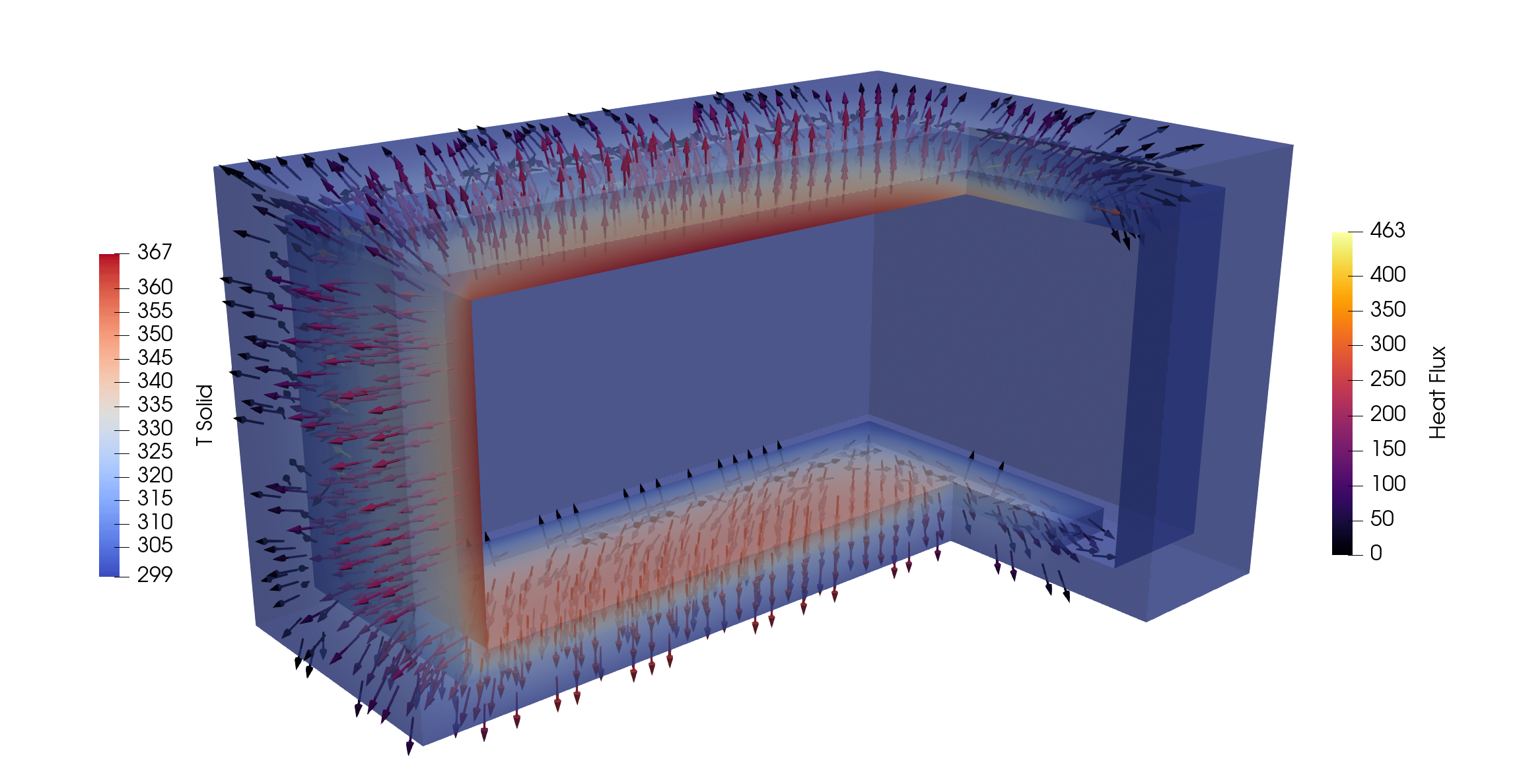
Step 6: Transient Heat Conduction
Executioner System
A system for dictating the simulation solving strategy.
Steady-state Executioner
Steady-state executioners generally solve the nonlinear system just once.
[Executioner]
  type = Steady
[]
The Steady executioner can solve the nonlinear system multiple times while adaptively refining the mesh to improve the solution.
Transient Executioners
Transient executioners solve the nonlinear system at least once per time step.
| Option | Definition |
|---|---|
dt | Starting time step size |
num_steps | Number of time steps |
start_time | The start time of the simulation |
end_time | The end time of the simulation |
scheme | Time integration scheme (discussed next) |
[Executioner]
  type = Transient
  scheme = 'implicit-euler'
  solve_type = 'PJFNK'
  start_time = 0.0
  num_steps = 5
  dt = 0.1
[]
Steady-State Detection
| Option | Definition |
|---|---|
steady_state_detection | Whether to try and detect achievement of steady-state (Default = false) |
steady_state_tolerance | Used for determining a steady-state; Compared against the difference in solution vectors between current and old time steps (Default = 1e-8) |
Common Executioner Options
There are a number of options that appear in the executioner block and are used to control the solver. Here are a few common options:
| Option | Definition |
|---|---|
l_tol | Linear Tolerance (default: 1e-5) |
l_max_its | Max Linear Iterations (default: 10000) |
nl_rel_tol | Nonlinear Relative Tolerance (default: 1e-8) |
nl_abs_tol | Nonlinear Absolute Tolerance (default: 1e-50) |
nl_max_its | Max Nonlinear Iterations (default: 50) |
Time Integrator System
A system for defining schemes for numerical integration in time.
The TimeIntegrator can be set using "scheme" parameter within the [Executioner] block, if the "type = Transient", the following options exist:
implicit-euler: Backward Euler (default)bdf2: Second order backward difference formulacrank-nicolson: Second order Crank-Nicolson methoddirk: Second order Diagonally-Implicit Runge-Kutta (DIRK)newmark-beta: Second order Newmark-beta method (structural dynamics)
TimeIntegrator Block
It is also possible to specify a time integrator as a separate sub-block within the input file. This allows for additional types and parameters to be defined, including custom TimeIntegrator objects.
[Executioner]
  type = Transient
  start_time = 0.0
  num_steps = 6
  dt = 0.1
  [TimeIntegrator]
    type = NewmarkBeta
    beta = 0.4225
    gamma = 0.8
  []
[]
Convergence Rates
Consider the test problem:
for , and , is chosen so the exact solution is given by and and are the initial and Dirichlet boundary conditions corresponding to this exact solution.

Time Stepper System
A system for computing time steps for transient executioners.
Built-in TimeSteppers
MOOSE includes many built-in TimeStepper objects:
ConstantDTSolutionTimeAdaptiveDTIterationAdaptiveDTFunctionDTPostprocessorDTTimeSequenceStepper
IterationAdaptiveDT
IterationAdaptiveDT grows or shrinks the time step based on the number of iterations taken to obtain a converged solution in the last converged step.
[Executioner]
  type = Transient
  solve_type = NEWTON
  start_time = 0.0
  dtmin = 1.0
  end_time = 10.0
  [TimeStepper]
    type = IterationAdaptiveDT
    optimal_iterations = 1
    linear_iteration_ratio = 1
    dt = 5.0
  []
[]
TimeSequenceStepper
Provide a vector of time points using parameter time_sequence, the object simply moves through these time points.
The and parameters are automatically added to the sequence.
Only time points satisfying are considered.
If a solve fails at step an additional time point is inserted and the step is resolved.
Composing TimeSteppers
New Feature: Time steppers can now be composed to follow complex time histories. By default, the minimum of all the time steps computed by all the time steppers is used!
What steps will be taken, starting at time = 0s?
[TimeSteppers]
  [constant]
    type = ConstantDT
    dt = 0.2
  []
  [hit_these_times]
    type = TimeSequenceStepper
    time_sequence = '0.5 1 1.5 2.1'
  []
[]
Step 6: Transient Heat Conduction
(continued)
To create a time-dependent problem add in the time derivative:
The time term exists in the heat transfer module as HeatConductionTimeDerivative.
Step 6: Time-dependent Input File
We introduce a time derivative kernel to model the contribution to the residual/Jacobian (and various time integration vectors) of the time derivative.
[Kernels]
  [diffusion_concrete]
    type = ADHeatConduction
    variable = T
  []
  [time_derivative]
    type = ADHeatConductionTimeDerivative
    variable = T
  []
[]
Time stepping parameters are passed to the Executioner block with the Transient executioner type.
[Executioner]
  type = Transient
  num_steps = 10
  dt = '${units 12 h -> s}'
  solve_type = NEWTON
  petsc_options_iname = '-pc_type -pc_hypre_type'
  petsc_options_value = 'hypre boomeramg'
[]
Step 6: Transient Simulation
There are generally two uses for time-dependent runs:
Transient: Performing a natural evolution of the model through time.
Pseudo-transient: Form of under-relaxation for a steady-state solve that more stably converges to the solution.
Material properties now include specific heat capacity and density for the time-derivative term.
HeatConductionMaterial has a parameter for the heat capacity.
GenericConstantMaterial is used to define the density.
 @@ -1,22 +1,43 @@
 [Materials]
   [concrete_hd]
     type = ADHeatConductionMaterial
     block = concrete_hd
     temp = 'T'
     # we specify a function of time, temperature is passed as the time argument
     # in the material
     thermal_conductivity_temperature_function = '5.0 + 0.001 * t'
+    specific_heat = 1050
   []
   [concrete]
     type = ADHeatConductionMaterial
     block = concrete
     temp = 'T'
     thermal_conductivity_temperature_function = '2.25 + 0.001 * t'
+    specific_heat = 1050
   []
   [Al]
     type = ADHeatConductionMaterial
     block = Al
     temp = T
     thermal_conductivity_temperature_function = '175'
+    specific_heat = 875
+  []
+  [density_concrete_hd]
+    type = ADGenericConstantMaterial
+    block = 'concrete_hd'
+    prop_names = 'density'
+    prop_values = '3524' # kg / m3
+  []
+  [density_concrete]
+    type = ADGenericConstantMaterial
+    block = 'concrete'
+    prop_names = 'density'
+    prop_values = '2403' # kg / m3
+  []
+  [density_Al]
+    type = ADGenericConstantMaterial
+    block = 'Al'
+    prop_names = 'density'
+    prop_values = '2270' # kg / m3
   []
 []
(+ tutorials/shield_multiphysics/inputs/step06_transient_heat_conduction/step6_transient.i)
Step 6: Running Transient Simulation
cd ~/projects/moose/tutorials/shield_multiphysics/inputs/step06_transient_heat_conduction
moose-opt -i step6_transient.i
Step 6: Transient Simulation Result
Step 6: Pseudo-Transient Simulation
Since the goal of a pseudo-transient is to achieve a steady state, the heat capacity (and density) do not matter and simply serve as relaxation factors. So in this example, we use a multiplier to reduce heat capacity to converge the steady-state solution faster:
cp_multiplier = 1e-6
 @@ -1,43 +1,43 @@
 [Materials]
   [concrete_hd]
     type = ADHeatConductionMaterial
     block = concrete_hd
     temp = 'T'
     # we specify a function of time, temperature is passed as the time argument
     # in the material
     thermal_conductivity_temperature_function = '5.0 + 0.001 * t'
-    specific_heat = 1050
+    specific_heat = '${fparse cp_multiplier * 1050}'
   []
   [concrete]
     type = ADHeatConductionMaterial
     block = concrete
     temp = 'T'
     thermal_conductivity_temperature_function = '2.25 + 0.001 * t'
-    specific_heat = 1050
+    specific_heat = '${fparse cp_multiplier * 1050}'
   []
   [Al]
     type = ADHeatConductionMaterial
     block = Al
     temp = T
     thermal_conductivity_temperature_function = '175'
-    specific_heat = 875
+    specific_heat = '${fparse cp_multiplier * 875}'
   []
   [density_concrete_hd]
     type = ADGenericConstantMaterial
     block = 'concrete_hd'
     prop_names = 'density'
     prop_values = '3524' # kg / m3
   []
   [density_concrete]
     type = ADGenericConstantMaterial
     block = 'concrete'
     prop_names = 'density'
     prop_values = '2403' # kg / m3
   []
   [density_Al]
     type = ADGenericConstantMaterial
     block = 'Al'
     prop_names = 'density'
     prop_values = '2270' # kg / m3
   []
 []
(+ tutorials/shield_multiphysics/inputs/step06_transient_heat_conduction/step6_pseudo_transient.i)
The Transient executioner has a steady_state_detection option to determine if the simulation has reached a steady-state:
 @@ -1,8 +1,9 @@
 [Executioner]
   type = Transient
-  num_steps = 10
-  dt = '${units 12 h -> s}'
+  steady_state_detection = true
   solve_type = NEWTON
   petsc_options_iname = '-pc_type -pc_hypre_type'
   petsc_options_value = 'hypre boomeramg'
+  # Difficult to converge with relative tolerance close to steady-state
+  nl_abs_tol = 1e-8
 []
(+ tutorials/shield_multiphysics/inputs/step06_transient_heat_conduction/step6_pseudo_transient.i)
Step 6: Running Pseudo-Transient Simulation
cd ~/projects/moose/tutorials/shield_multiphysics/inputs/step06_transient_heat_conduction
moose-opt -i step6_pseudo_transient.i
Step 6: Pseudo-Transient Simulation Result
Step 7: Mechanics
Mechanics
Compute the elastic and thermal strain if the shield is only held on the ground surface:
where:
is the Cauchy stress tensor
is an additional source of stress
is the displacement vector
is the body force (here, gravity)
is the unit normal to the boundary
is the prescribed displacement on the boundary (here, the ground)
is the prescribed traction on the boundary (here, none)
Thermal expansion causes additional strain.
Modules
Chemical Reactions
Provides a set of tools for the calculation of multicomponent aqueous reactive transport in porous media, originally developed as the MOOSE application RAT (Guo et al., 2013).
Contact
Provides the necessary tools for modeling mechanical contact using algorithms to enforce constraints between surfaces in the mesh, to prevent penetration and develop contact forces.
Contact: Frictional Ironing Problem
Frictional ironing model using mortar contact.
Electromagnetics
The Electromagnetics module provides components and models to simulate electromagnetic wave problems using MOOSE, and facilitate coupling of electromagnetic simulations to other physical domains. Maxwell's equations are solved for complex fields using a Helmholtz wave equation formulation in 1-D and 2-D. Electrostatic contact is also provided for imperfect electric interfaces.
Electric field radiation pattern of half-wave dipole antenna.
External PETSc Solver
Provides support for stand-alone native PETSc applications that are to be coupled with moose-based applications. It is also a general example for coupling to an external application.
Fluid Properties
The Fluid Properties module provides a consistent interface to fluid properties such as density, viscosity, enthalpy and many others, as well as derivatives with respect to the primary variables. The consistent interface allows different fluids to be used in an input file by simply swapping the name of the Fluid Properties UserObject in a plug-and-play manner.
Fluid-Structure Interaction
Provides tools that solve fluid and structure problems, wherein, their behavior is inter-dependent. Currently capable of simulating fluid-structure interaction behavior using an acoustic formulation for the fluid.

Sloshing in an advanced reactor vessel
Functional Expansion Tools
A MOOSE module for continuous, mesh-agnostic, high-fidelity, reduced-data MultiApp coupling
Functional expansions (FXs) are a methodology that represent information as moments of a functional series (Flusser et al., 2016). This is related to a Fourier series representation of cyclic data. Moments are generated via numerical integration for each term in the functional series to represent the field of interest. These moments can then be used to reconstruct the field in a separate app (Wendt et al., 2018; Wendt and Kerby, 2017; Kerby et al., 2017).
Geochemistry
Solves geochemical models. The capabilities include:
Equilibrium aqueous systems
Redox disequilibrium
Sorption and surface complexation
Kinetics
All of the above combined with fluid and heat transport
It is designed to interface easily with the porous flow module so that complicated reactive transport scenarios can be studied.
Heat Transfer
Basic utilities for solving the transient heat conduction equation:
Also contains capability for generalized heat transfer (convection, radiation, ...).
Level Set
The level set module provides basic functionality to solve the level set equation, which is simply the multi-dimensional advection equation:
Navier Stokes
A library for the implementation of simulation tools that solve the multi-dimensional Navier-Stokes equations using either the continuous Galerkin finite element (CGFE) or the finite volume (FV) method. The Navier-Stokes equations may be solved with:
An incompressible formulation (CGFE & FV)
A weakly compressible formulation (FV)
A fully compressible formulation (FV)
Zero-dimensional turbulence models are available and coarse regularized k-epsilon will be added soon.
Navier Stokes
Flow in a lid-driven cavity with Re=417 (left) and Re=833 (right).


Optimization
The MOOSE optimization module provides functionality for solving inverse optimization problems in MOOSE. It is based on PDE constrained optimization using the PETSc TAO optimization solver.

Figure 1: Optimization cycle example for parameterizing an internal heat source distribution to match the simulated and experimental temperature field, and , respectively.
Phase Field
The MOOSE phase field module is a library for simplifying the implementation of simulation tools that employ the phase field model.
Porous Flow
The PorousFlow module is a library of physics for fluid and heat flow in porous media. It is formulated in an extremely general manner, so is capable of solving problems with an arbitrary number of phases (gas, liquid, etc) and fluid components (species present in each fluid phase), using any set of primary variables.
Ray Tracing
Provides capability for tracing rays through a finite element mesh. Notable features include:
Contribution to residuals and Jacobians from along a ray
Ray interaction with internal and external boundaries
Supports storage and manipulation of data unique to each ray
Supports ray interaction with field variables
Highly parallelizable: tested to 20k MPI ranks
Ray Tracing: Flashlight source

Example of flashlight point sources within a diffusion-reaction problem

Overlay of the rays used within the problem on the left
Reconstructed Discontinuous Galerkin (rDG)
The MOOSE rDG module is a library for the implementation of simulation tools that solve convection-dominated problems using the class of so-called reconstructed discontinuous Galerkin (rDG) methods. The specific rDG method implemented in this module is rDG(P0P1), which is equivalent to the second-order cell-centered finite volume method (FVM).
Reactor
Adds advanced meshing capabilities to MOOSE so that users can create complex-geometry meshes related to the structures of reactor cores. This includes:
Creating and modifying hexagonal mesh components for assemblies
Stitching assemblies together to form core meshes
Creating peripheral regions for assemblies and cores
Adding IDs for pins and assembly regions
Enabling the dynamic and static simulation of rotational control drums.
Reactor: Meshing a Microreactor

Meshing a microreactor in stages using the Reactor module: from pins and control drums to assemblies, cores, and peripheral regions.
Stochastic Tools
A toolbox designed for performing stochastic analysis for MOOSE-based applications. Capabilities include:
Parameter Studies
Sensitivity Analysis
Uncertainty Quantification
Surrogate/Reduced-Order Model generation

Solid Mechanics
The Solid Mechanics module is a library of simulation tools that solve continuum mechanics problems. The module can be used to simulation both linear and finite strain mechanics, including Elasticity and Cosserat elasticity, Plasticity and micromechanics plasticity, Creep, and Damage due to cracking and property degradation.
Thermal Hydraulics
The Thermal Hydraulics module is a library of components that can be used to build thermal-hydraulic simulations. Basic capabilities include a 1-phase, variable-area, inviscid, compressible flow model with a non-condensable vapor mixture, 2-D and 3-D heat conduction, a control logic system, and pluggable closure systems and models.
Extended Finite Element Method (XFEM)
A MOOSE-based implementation of the extended finite element method, which is a numerical method that is especially designed for treating discontinuities.
Mesh system (continued)
Replicated Mesh
When running in parallel the default mode for operation is to use a replicated mesh, which creates a complete copy of the mesh for each processor.
[Mesh]
  parallel_type = replicated
[]
Distributed Mesh
Changing the type to distributed when running in parallel operates such that only the portion of the mesh owned by a processor is stored on that processor.
[Mesh]
  parallel_type = distributed
[]
If the mesh is too large to read in on a single processor, it can be split prior to the simulation.
Copy the mesh to a large memory machine
Use the
--split-meshoption to split the mesh into piecesRun the executable with
--use-split
Displaced Mesh
Calculations can take place in either the initial mesh configuration or, when requested, the "displaced" configuration.
To enable displacements, provide a vector of displacement variable names for each spatial dimension in the Mesh block.
[Mesh]
  [gen]
    type = GeneratedMeshGenerator
    dim = 2
    xmin = 0
    ymin = 0
    xmax = 0.2
    ymax = 0.5
    nx = 5
    ny = 15
    elem_type = QUAD4
  []
  displacements = 'disp_x disp_y'
[]
Objects can enforce the use of the displaced mesh within the validParams function.
params.set<bool>("use_displaced_mesh") = true;
Step 7: Mechanics
(continued)
Step 7: Input File
We utilize the custom syntax (more on this in Step 12) to automatically add the necessary objects (Variables, Kernels, Materials, etc.) for this problem: Physics/SolidMechanics/QuasiStatic
[Mesh]
  [fmg]
    type = FileMeshGenerator
    file = '../step03_boundary_conditions/mesh_in.e'
  []
[]

[GlobalParams]
  displacements = 'disp_x disp_y disp_z'
[]

[Variables]
  [T]
    # Adds a Linear Lagrange variable by default
    block = 'concrete_hd concrete Al'
  []
[]

[Kernels]
  [diffusion_concrete]
    type = ADHeatConduction
    variable = T
  []

  [gravity]
    type = Gravity
    variable = 'disp_z'
    value = '-9.81'
    block = 'concrete_hd concrete Al'
  []
[]

[Physics/SolidMechanics/QuasiStatic]
  [all]
    # This block adds all of the proper Kernels, strain calculators, and Variables
    # for Solid Mechanics equations in the correct coordinate system (autodetected)
    add_variables = true
    strain = FINITE
    eigenstrain_names = eigenstrain
    use_automatic_differentiation = true
    generate_output = 'vonmises_stress elastic_strain_xx elastic_strain_yy strain_xx strain_yy'
    block = 'concrete_hd concrete Al'
  []
[]

[BCs]
  [from_reactor]
    type = NeumannBC
    variable = T
    boundary = inner_cavity_solid
    # 5 MW reactor, only 50 kW removed from radiation, 144 m2 cavity area
    value = '${fparse 5e4 / 144}'
  []
  [air_convection]
    type = ADConvectiveHeatFluxBC
    variable = T
    boundary = 'air_boundary'
    T_infinity = 300.0
    # The heat transfer coefficient should be obtained from a correlation
    heat_transfer_coefficient = 10
  []
  [ground]
    type = DirichletBC
    variable = T
    value = 300
    boundary = 'ground'
  []
  [water_convection]
    type = ADConvectiveHeatFluxBC
    variable = T
    boundary = 'water_boundary_inwards'
    T_infinity = 300.0
    # The heat transfer coefficient should be obtained from a correlation
    heat_transfer_coefficient = 600
  []

  [hold_ground_x]
    type = DirichletBC
    variable = disp_x
    boundary = ground
    value = 0
  []
  [hold_ground_y]
    type = DirichletBC
    variable = disp_y
    boundary = ground
    value = 0
  []
  [hold_ground_z]
    type = DirichletBC
    variable = disp_z
    boundary = ground
    value = 0
  []
[]

[Materials]
  [concrete_hd]
    type = ADHeatConductionMaterial
    block = concrete_hd
    temp = 'T'
    # we specify a function of time, temperature is passed as the time argument
    # in the material
    thermal_conductivity_temperature_function = '5.0 + 0.001 * t'
  []
  [concrete]
    type = ADHeatConductionMaterial
    block = concrete
    temp = 'T'
    thermal_conductivity_temperature_function = '2.25 + 0.001 * t'
  []
  [Al]
    type = ADHeatConductionMaterial
    block = Al
    temp = T
    thermal_conductivity_temperature_function = '175'
  []

  [elasticity_tensor_concrete_hd]
    type = ADComputeIsotropicElasticityTensor
    youngs_modulus = 2.75e9 # (Pa)
    poissons_ratio = 0.15
    block = 'concrete_hd'
  []
  [elasticity_tensor_concrete]
    type = ADComputeIsotropicElasticityTensor
    youngs_modulus = 30e9 # (Pa)
    poissons_ratio = 0.2
    block = 'concrete'
  []
  [elasticity_tensor_Al]
    type = ADComputeIsotropicElasticityTensor
    youngs_modulus = 68e9 # (Pa)
    poissons_ratio = 0.36
    block = 'Al'
  []

  [elastic_stress]
    type = ADComputeFiniteStrainElasticStress
    block = 'concrete_hd concrete Al'
  []

  [thermal_strain_concrete_hd]
    type = ADComputeThermalExpansionEigenstrain
    stress_free_temperature = 300
    eigenstrain_name = eigenstrain
    temperature = T
    thermal_expansion_coeff = 1e-5 # 1/K
    block = 'concrete_hd'
  []
  [thermal_strain_concrete]
    type = ADComputeThermalExpansionEigenstrain
    stress_free_temperature = 300
    eigenstrain_name = eigenstrain
    temperature = T
    thermal_expansion_coeff = 1e-5 # 1/K
    block = 'concrete'
  []
  [thermal_strain_Al]
    type = ADComputeThermalExpansionEigenstrain
    stress_free_temperature = 300 # arbitrary value
    eigenstrain_name = eigenstrain
    temperature = T
    thermal_expansion_coeff = 2.4e-5 # 1/K
    block = 'Al'
  []

  # NOTE: This handles thermal expansion by coupling to the displacements
  [density_concrete_hd]
    type = Density
    block = 'concrete_hd'
    density = '3524' # kg / m3
  []
  [density_concrete]
    type = Density
    block = 'concrete'
    density = '2403' # kg / m3
  []
  [density_Al]
    type = Density
    block = 'Al'
    density = '2270' # kg / m3
  []
[]

[Problem]
  # No kernels on the water domain
  kernel_coverage_check = false
  # No materials defined on the water domain
  material_coverage_check = false
[]

[Executioner]
  type = Steady

  solve_type = NEWTON
  automatic_scaling = true

  petsc_options_iname = '-pc_type -pc_hypre_type -ksp_gmres_restart'
  petsc_options_value = 'hypre boomeramg 500'
  line_search = none
[]

[Outputs]
  exodus = true
[]
Step 7: Run
cd ~/projects/moose/tutorials/shield_multiphysics/inputs/step07_mechanics
moose-opt -i step7.i
Step 7: Result
Displacements are exaggerated to be visible.
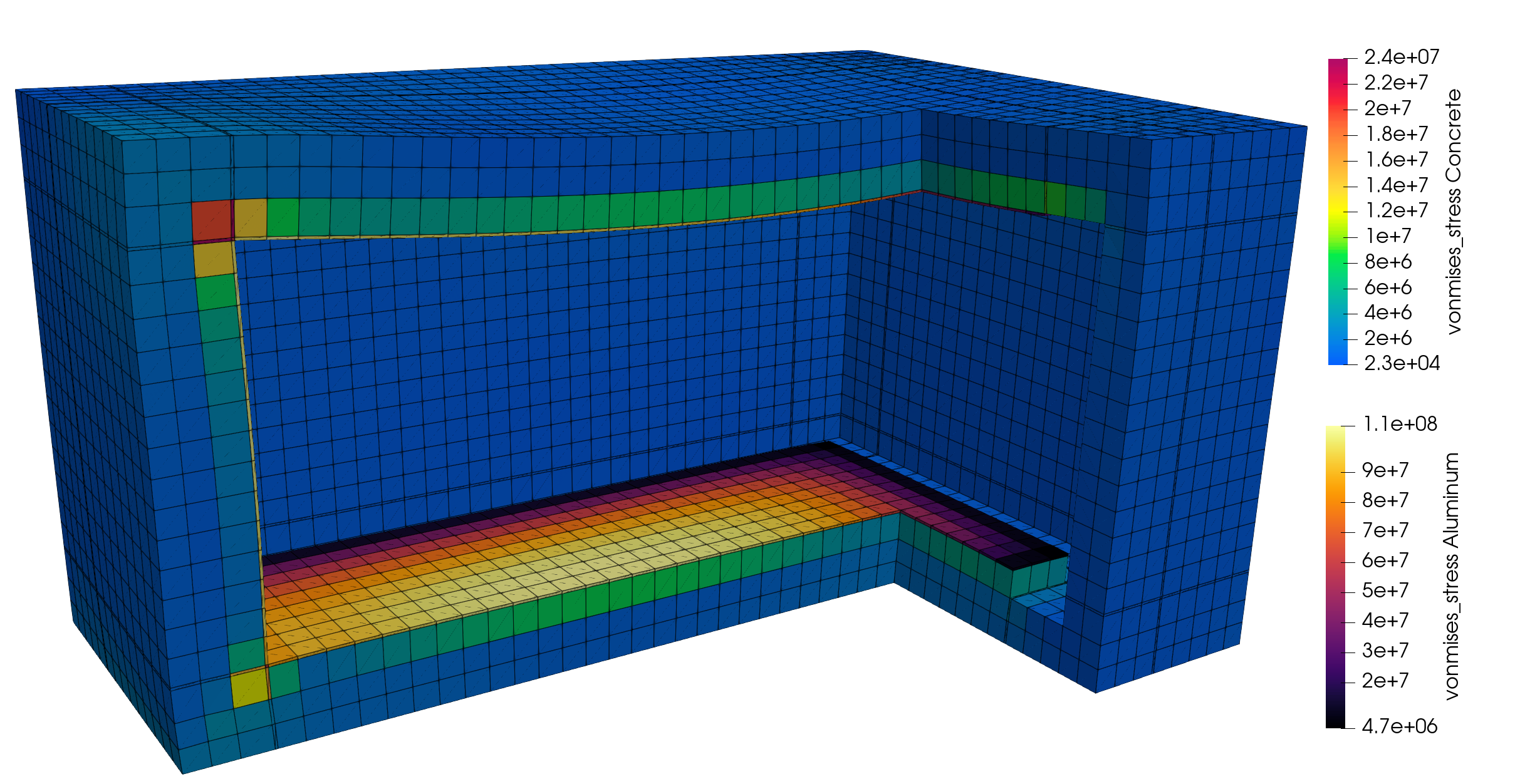
Step 8: Mesh Adaptivity
Adaptivity System
h-Adaptivity
-adaptivity is a method of automatically refining/coarsening the mesh in regions of high/low estimated solution error.
Concentrate degrees of freedom (DOFs) where the error is highest, while reducing DOFs where the solution is already well-captured.
Compute a measure of error using an
IndicatorobjectMark an element for refinement or coarsening based on the error using a
Markerobject
Mesh adaptivity can be employed in both Steady and Transient executioners.
Refinement Patterns
MOOSE employs "self-similar", isotropic refinement patterns: when refining an element is split into elements of the same type.
For example, when using Quad4 elements, four "child" elements are created when the element is refined.
Coarsening happens in reverse, children are deleted and the "parent" element is reactivated.
The original mesh starts at refinement level 0.

Indicator Objects
Indicators report an amount of "error" for each element, built-in Indicators include:
GradientJumpIndicator
Jump in the gradient of a variable across element edges. A good "curvature" indicator that works well over a wide range of problems.
FluxJumpIndicator
Similar to GradientJump, except that a scalar coefficient (e.g. thermal conductivity) can be provided to produce a physical "flux" quantity.
LaplacianJumpIndicator
Jump in the second derivative of a variable. Only useful for shape functions.
AnalyticIndicator
Computes the difference between the finite element solution and a user-supplied Function representing the analytic solution to the problem.
Marker Objects
After an Indicator has computed the error for each element, a decision to refine or coarsen elements must be made using a Marker object.
ErrorFractionMarker
Selects elements based on their contribution to the total error.
ErrorToleranceMaker
Refine if error is greater than a specified value and coarsen if it is less.
ValueThresholdMarker
Refine if variable value is greater than a specific value and coarsen if it is less.
BoxMarker
Refine or coarsen inside or outside a given box.
ComboMarker
Combine several of the above Markers.
Input Syntax
[Adaptivity]
  initial_steps = 2
  cycles_per_step = 2
  marker = marker
  initial_marker = marker
  max_h_level = 2
  [Indicators]
    [indicator]
      type = GradientJumpIndicator
      variable = u
    []
  []
  [Markers]
    [marker]
      type = ErrorFractionMarker
      indicator = indicator
      coarsen = 0.1
      refine = 0.7
    []
  []
[]
Step 8: Mesh Adaptivity
(continued)
Step 8: Uniform Refinement
 @@ -1,6 +1,7 @@
 [Mesh]
   [fmg]
     type = FileMeshGenerator
     file = '../step03_boundary_conditions/mesh_in.e'
   []
+  uniform_refine = 0
 []
(+ tutorials/shield_multiphysics/inputs/step08_adaptivity/step8_uniform.i)
Step 8: Run coarse problem
Without modification, running the input will produce the same solution as in Step 4:
cd ~/projects/moose/tutorials/shield_multiphysics/inputs/step08_adaptivity
moose-opt -i step8_uniform.i
Step 8: Run Uniform Refinement
There are several ways to instigate uniform refinement:
Directly modify the input to change
uniform_refine = 0touniform_refine = 2Modify parameter using command-line interface:
moose-opt -i step8_uniform.i Mesh/uniform_refine=2Use the
-rcommand-line option:moose-opt -i step8_uniform.i -r 2
Each refinement increases the number of elements by a factor of
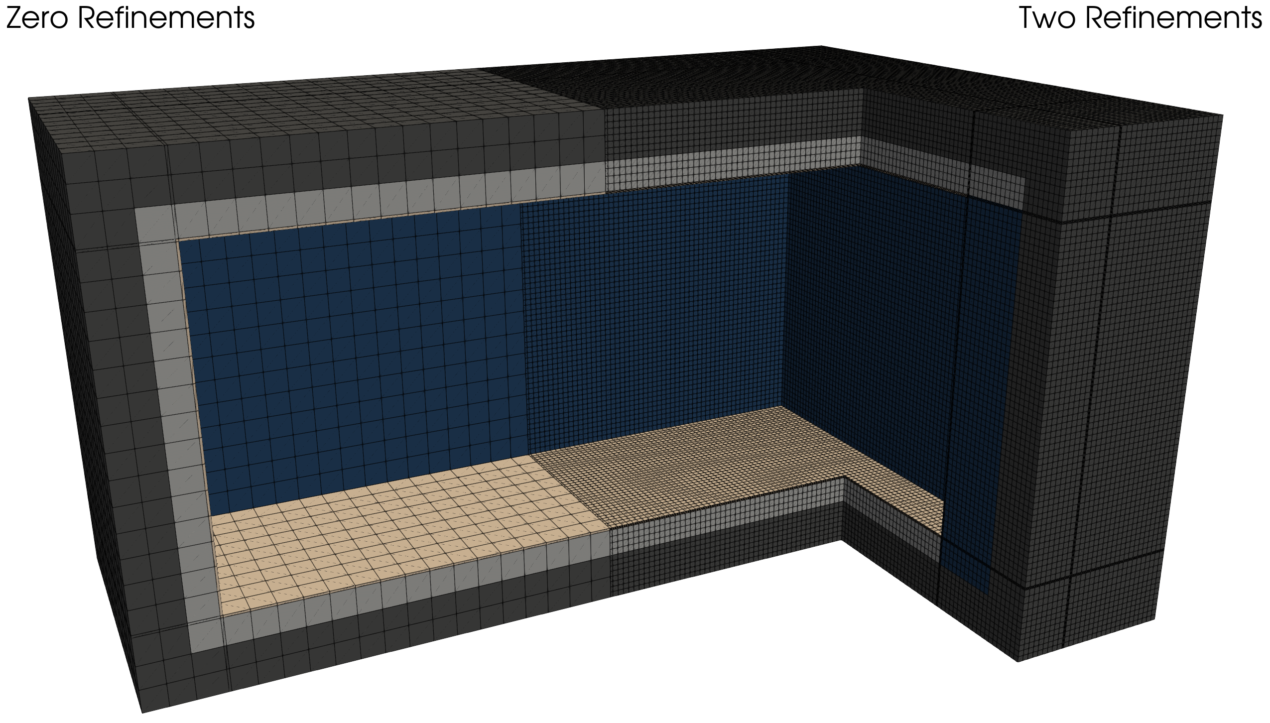
Step 8: Mesh Adaptivity
The Adaptivity System is used to perfrom adaptive mesh refinement.
Indicators provide a measure of the error in the simulation, see GradientJumpIndicator.
Markers flag elements for refinement or coarsening, see ValueThresholdMarker
[Adaptivity]
  marker = jump_threshold
  max_h_level = 2
  [Indicators]
    [temperature_jump]
      type = GradientJumpIndicator
      variable = T
      scale_by_flux_faces = true
    []
  []
  [Markers]
    [jump_threshold]
      type = ValueThresholdMarker
      coarsen = 0.3
      variable = temperature_jump
      refine = 2
      block = 'concrete_hd concrete Al'
    []
  []
[]
Step 8c: Run Mesh Adaptivity
moose-opt -i step8_adapt.i
Step 9: Postprocessors
Aggregate values based on simulation data are useful for understanding the simulation as well as defining coupling values across coupled equations.
There are two main systems for aggregating data: Postprocessors and VectorPostprocessors.
All MOOSE Postprocessors are based on the UserObject System, so we will begin with an introduction there.
UserObject System
A system for defining an arbitrary interface between MOOSE objects.
The UserObject system provides data and calculation results to other MOOSE objects.
Postprocessors are UserObjects that compute a single scalar value.
VectorPostprocessors are UserObjects that compute vectors of data.
UserObjects define their own interface, which other MOOSE objects can call to retrieve data.
Execution
UserObjects are computed at specified "times" by the execute_on option in the input file:
execute_on = 'initial timestep_end'execute_on = linearexecute_on = nonlinearexecute_on = 'timestep_begin final failed'
They can be restricted to specific blocks, sidesets, and nodesets
Postprocessor System
A system for computing a "reduction" or "aggregation" calculation based on the solution variables that results in a single scalar value.
Types of Postprocessors
The operation defined in the ::compute... routine is applied at various locations depending on the Postprocessor type.
ElementPostprocessor: operates on each element
NodalPostprocessor: operates on each node
SidePostprocessor: operates on each element side on a boundary
InternalSidePostprocessor: operates on internal element sides
InterfacePostprocessor: operates on each element side on subdomain interfaces
GeneralPostprocessor: operates once per execution
Built-in Postprocessor Types
MOOSE includes a large number built-in Postprocessors: ElementAverageValue, SideAverageValue, ElementL2Error, ElementH1Error, and many more
By default, Postprocessors will output to a formatted table on the screen and optionally using the [Outputs] block be stored in CSV file.
[Output]
  csv = true
[]
VectorPostprocessor System
A system for "reduction" or "aggregation" calculations based on the solution variables that results in one or many vectors of values.
Built-in VectorPostprocessor Types
MOOSE includes a large number built-in VectorPostprocessors: NodalValueSampler, LineValueSampler, PointValueSampler, and many more.
VectorPostprocessors output is optionally enabled using the [Outputs] block. A CSV file for each vector and timestep will be created.
[Output]
  csv = true
[]
Step 9: Postprocessors
(continued)
Step 9: Input File
Postprocessors and VectorPostprocessors in this example:
!include ../step08_adaptivity/step8_adapt.i

[Postprocessors]
  [num_elements]
    type = NumElements
    execute_on = 'INITIAL TIMESTEP_END'
  []
  [max_temperature_concrete]
    type = NodalExtremeValue
    variable = T
    block = 'concrete_hd concrete'
    value_type = max
    execute_on = 'INITIAL TIMESTEP_END'
  []
  [water_heat_flux]
    type = ADSideDiffusiveFluxIntegral
    variable = T
    boundary = water_boundary_inwards
    diffusivity = 'thermal_conductivity'
  []
[]

[VectorPostprocessors]
  [temperature_sample_x]
    type = LineValueSampler
    num_points = 50
    start_point = '1.275 4.625 0.8'
    end_point = '5.275 4.625 0.8'
    variable = T
    sort_by = x
    execute_on = 'INITIAL TIMESTEP_END'
  []
  [temperature_sample_y]
    type = LineValueSampler
    num_points = 50
    start_point = '3.275 0.825 0.8'
    end_point = '3.275 8.425 0.8'
    variable = T
    sort_by = y
    execute_on = 'INITIAL TIMESTEP_END'
  []
[]

[Outputs]
  csv = true
[]
Step 9: Run
cd ~/projects/moose/tutorials/shield_multiphysics/inputs/step09_postprocessing
moose-opt -i step9.i
Then plot from the CSV file in python, excel, paraview etc
To have non-zero values at t=0, the postprocessors must be executed on INITIAL.
Postprocessor Values:
+----------------+--------------------------+----------------+----------------+
| time           | max_temperature_concrete | num_elements   | water_heat_flux|
+----------------+--------------------------+----------------+----------------+
|   0.000000e+00 |             3.000000e+02 |   1.792000e+04 |   0.000000e+00 |
|   4.320000e+04 |             3.226249e+02 |   1.792000e+04 |   5.445889e+03 |
|   8.640000e+04 |             3.348682e+02 |   2.436000e+04 |   7.445028e+03 |
|   1.296000e+05 |             3.416370e+02 |   3.379600e+04 |   8.692277e+03 |
|   1.728000e+05 |             3.464075e+02 |   3.491600e+04 |   9.406888e+03 |
|   2.160000e+05 |             3.500610e+02 |   3.519600e+04 |   9.912671e+03 |
+----------------+--------------------------+----------------+----------------+
Step 9: Visualization using Plotly
#!/usr/bin/env python3
# * This file is part of the MOOSE framework
# * https://www.mooseframework.org
# *
# * All rights reserved, see COPYRIGHT for full restrictions
# * https://github.com/idaholab/moose/blob/master/COPYRIGHT
# *
# * Licensed under LGPL 2.1, please see LICENSE for details
# * https://www.gnu.org/licenses/lgpl-2.1.html

import os
import shutil
import mooseutils

import plotly.graph_objects as go

def run():
    exec = shutil.which("moose-opt") or mooseutils.find_moose_executable_recursive()
    if not exec:
        raise AssertionError("Cannot find a valid MOOSE executable.")
    mooseutils.run_executable(exec, ["-i", "step9.i"])

def plot():
    pp_data = mooseutils.PostprocessorReader("step9_out.csv")
    times = pp_data["time"]
    time_hrs = times / 3600

    fig = go.Figure(
        data=go.Scatter(
            x=time_hrs,
            y=pp_data["max_temperature_concrete"] - 273,
        )
    )
    fig.update_layout(
        xaxis=dict(title=dict(text="Time (hours)")),
        yaxis=dict(title=dict(text="Concrete Max Temperature (C)")),
    )
    fig.show()

    fig = go.Figure(
        data=go.Scatter(
            x=time_hrs,
            y=pp_data["water_heat_flux"] / 1000,
        )
    )
    fig.update_layout(
        xaxis=dict(title=dict(text="Time (hours)")),
        yaxis=dict(title=dict(text="Water heat flux (kW/m2)")),
    )
    fig.show()

    vpp_data_x = mooseutils.VectorPostprocessorReader(
        "step9_out_temperature_sample_x_*.csv"
    )
    vpp_data_y = mooseutils.VectorPostprocessorReader(
        "step9_out_temperature_sample_y_*.csv"
    )

    figx = go.Figure()
    figy = go.Figure()
    for it in vpp_data_x.times()[::2]:
        vpp_data_x.update(it)
        vpp_data_y.update(it)

        label = f"Time = {int(time_hrs[it] / 24)} days"
        figx.add_trace(
            go.Scatter(x=vpp_data_x["x"], y=vpp_data_x["T"] - 273, name=label)
        )
        figy.add_trace(
            go.Scatter(x=vpp_data_y["y"], y=vpp_data_y["T"] - 273, name=label)
        )

    figx.update_layout(
        xaxis=dict(title=dict(text="x (m)")),
        yaxis=dict(title=dict(text="Temperature (C)")),
    )
    figy.update_layout(
        xaxis=dict(title=dict(text="y (m)")),
        yaxis=dict(title=dict(text="Temperature (C)")),
    )

    figx.show()
    figy.show()

if __name__ == "__main__":
    if not os.path.exists("step9_out.csv"):
        run()
    plot()
Ensure the MOOSE python utilities are in the PYTHONPATH:
export PYTHONPATH=$PYTHONPATH:$HOME/projects/moose/python
python step9.py
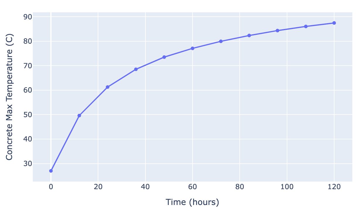
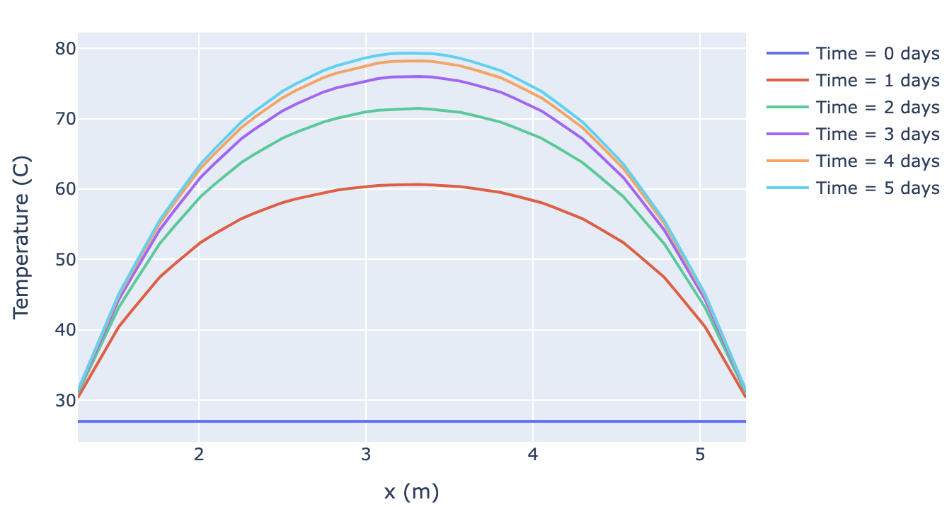
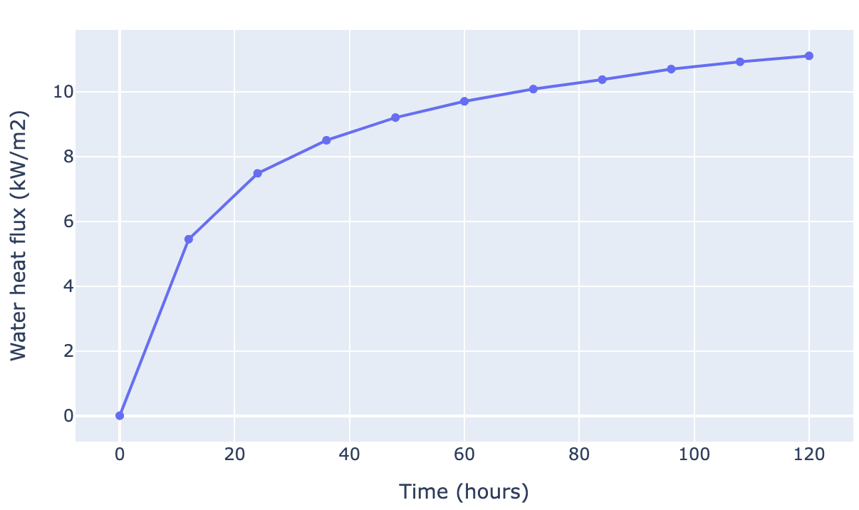
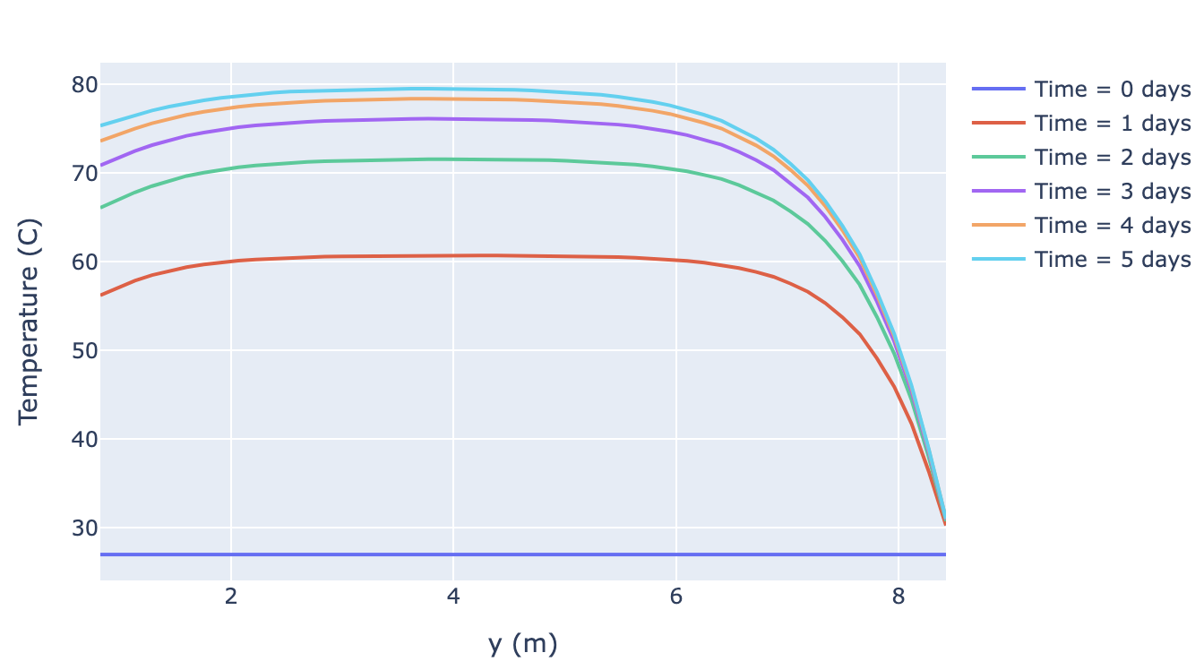
Step 10: Finite Volume
We have only solved the heat equation in the concrete until now. We want to model natural circulation in the water tank inside the shield.
Conservation of Mass:
(17)Conservation of momentum:
(18)Conservation of Energy:
(19)where is the fluid velocity, is fluid viscosity, is the pressure, is the density, is the gravity vector, and is the temperature.
Finite Volume Method (FVM)
Advantages of Finite Volume Method
(1) Flexible: Works with arbitrary mixed cell types (even if they are mixed in the same problem)
(2) Inherently conservative: Uses the integral form of the PDEs. This makes it perfect for applications where conservation laws need to be respected (fluid flows).
(3) Accurate: Can be second-order accurate in space. Higher order possible, but not common.
(4) Robust: It is the current standard for most commercial (STAR-CCM+, ANSYS-Fluent, etc.) and major open-source (OpenFOAM, etc.) CFD codes.
(5) Rich literature: Has been researched for decades.
Approximating the Solution
First, domain is split into cells ().

In MOOSE, the cell-centered finite volume approximation (Moukalled et al. (2016) and Jasak (1996)) is used due to the fact that it supports both unstructured and structured meshes:
Constant over the cells (value at cell centroid): if
Constant over the faces (value at face centroid): if
Error analysis is done using Taylor expansions, we prefer second-order discretization/interpolation schemes.
FVM using an Advection-Diffusion-Reaction Problem
(1) Write the strong form of the equation:
(2) Integrate the equation over the domain :
(3) Split the integral into different terms:
Approximating the Reaction and Source Terms
Split into cell-wise integrals:
Use the finite volume approximation (on cell C):
Approximating the Diffusion Term
Othogonal scenario: ( and are parallel)

Non-othogonal scenario:

Split into cell-wise integrals and use the divergence theorem:
On an internal cell (let's say on cell C):
for orthogonal scenario: (cheap and accurate)
for nonorthogonal scenario:
The surface normal () is expanded into a -parallel () and a remaining vector ():
on the right hand side is computed using the interpolation of cell gradients (next slide)
Interpolation and Gradient Estimation
Basic interpolation scheme:

Cell gradients can be estimated using the Green-Gauss theorem:
At the same time:
From the two equations:
(Alternative approaches: least-squares, node-based interpolation, skewness-corrected interpolation)
Approximating the Advection Term
Split to integral to cell-wise integrals and use the divergence theorem:
On an internal cell (let's say on cell C), assuming that is constant:
Common interpolation method for :
Upwind
(Weighted) Average
TVD limited schemes: van Leer, Minmod
The MOOSE Functor System
Unifies the evaluation of Functions, Variables, and certain Materials on faces, elements, quadrature points, etc.
Can be used to easily evaluate gradients on elements/faces as well.
They require an argument that contains information on the way the value should be obtained:
ElemArg: used to evaluate on an element, contains a link to the underlying element inlibMeshFaceArg: used to evaluate on a face, has to contains information about the face, surrounding elements and the interpolation method
auto elem_arg = ElemArg{elem.get(), false};
auto face = FaceArg({&fi, LimiterType::CentralDifference, true, false, nullptr, nullptr});
test_gradient(face);
Example Input File
a=1.1
diff=1.1

[Mesh]
  [./gen_mesh]
    type = GeneratedMeshGenerator
    dim = 2
    xmin = 2
    xmax = 3
    ymin = 0
    ymax = 1
    nx = 2
    ny = 2
    elem_type = TRI3
  [../]
[]

[Variables]
  [v]
    type = MooseVariableFVReal
    initial_condition = 1
  []
[]

[FVKernels]
  [advection]
    type = FVAdvection
    variable = v
    velocity = '${a} ${fparse 2*a} 0'
    advected_interp_method = 'average'
  []
  [reaction]
    type = FVReaction
    variable = v
  []
  [diff_v]
    type = FVDiffusion
    variable = v
    coeff = ${diff}
  []
  [body_v]
    type = FVBodyForce
    variable = v
    function = 'forcing'
  []
[]

[FVBCs]
  [exact]
    type = FVFunctionDirichletBC
    boundary = 'left right top bottom'
    function = 'exact'
    variable = v
  []
[]

[Functions]
  [exact]
    type = ParsedFunction
    expression = 'sin(x)*cos(y)'
  []
  [forcing]
    type = ParsedFunction
    expression = '-2*a*sin(x)*sin(y) + a*cos(x)*cos(y) + 2*diff*sin(x)*cos(y) + sin(x)*cos(y)'
    symbol_names = 'a diff'
    symbol_values = '${a} ${diff}'
  []
[]

[Executioner]
  type = Steady
  solve_type = 'NEWTON'
[]

[Outputs]
  csv = true
[]

[Postprocessors]
  [error]
    type = ElementL2Error
    variable = v
    function = exact
    outputs = 'console csv'
    execute_on = 'timestep_end'
  []
  [h]
    type = AverageElementSize
    outputs = 'console csv'
    execute_on = 'timestep_end'
  []
[]
Application in the Navier Stokes Module of MOOSE
Focuses on coarse-mesh applications
Supports free and porous medium flows
Supports incompressible, weakly-compressible and (some) compressible simulations
Under intense development
To the right: cooling of a spent fuel cask with natural circulation (Results by Sinan Okyay)

Step 10: Finite Volume
(continued)
Step 10: Natural convection
We introduce the Boussinesq approximation:
We set up the flow equations:
cp_water_multiplier = 5e-2
mu_multiplier = 1
power = '${fparse 5e4 / 144}'

[Mesh]
  [fmg]
    type = FileMeshGenerator
    file = 'mesh2d_in.e'
  []
[]

[Variables]
  [vel_x]
    type = INSFVVelocityVariable
    block = 'water'
    initial_condition = 1e-4
  []
  [vel_y]
    type = INSFVVelocityVariable
    block = 'water'
    initial_condition = 1e-4
  []
  [pressure]
    type = INSFVPressureVariable
    block = 'water'
    initial_condition = 1e5
  []
  [T_fluid]
    type = INSFVEnergyVariable
    initial_condition = 300
    block = 'water'
    scaling = 1e-05
  []
  [lambda]
    type = MooseVariableScalar
    family = SCALAR
    order = FIRST
  []
[]

[AuxVariables]
  # This isn't used in simulation, but useful for visualization
  [vel_z]
    type = INSFVVelocityVariable
    block = 'water'
    initial_condition = 0
  []
  [mixing_length]
    block = 'water'
    order = CONSTANT
    family = MONOMIAL
    fv = true
  []
[]

[GlobalParams]
  velocity_interp_method = rc
  rhie_chow_user_object = ins_rhie_chow_interpolator
  rho = rho
[]

[FVKernels]
  [water_ins_mass_advection]
    type = INSFVMassAdvection
    advected_interp_method = upwind
    block = water
    variable = pressure
  []
  [water_ins_mass_pressure_pin]
    type = FVPointValueConstraint
    lambda = lambda
    phi0 = 1e5
    point = '1 3 0'
    variable = pressure
  []
  [water_ins_momentum_time_vel_x]
    type = INSFVMomentumTimeDerivative
    block = water
    momentum_component = x
    variable = vel_x
  []
  [water_ins_momentum_time_vel_y]
    type = INSFVMomentumTimeDerivative
    block = water
    momentum_component = y
    variable = vel_y
  []
  [water_ins_momentum_advection_x]
    type = INSFVMomentumAdvection
    advected_interp_method = upwind
    block = water
    momentum_component = x
    variable = vel_x
    characteristic_speed = 0.01
  []
  [water_ins_momentum_advection_y]
    type = INSFVMomentumAdvection
    advected_interp_method = upwind
    block = water
    momentum_component = y
    variable = vel_y
    characteristic_speed = 0.1
  []
  [water_ins_momentum_diffusion_x]
    type = INSFVMomentumDiffusion
    block = water
    momentum_component = x
    mu = mu
    variable = vel_x
  []
  [water_ins_momentum_diffusion_y]
    type = INSFVMomentumDiffusion
    block = water
    momentum_component = y
    mu = mu
    variable = vel_y
  []
  [water_ins_momentum_pressure_x]
    type = INSFVMomentumPressure
    block = water
    momentum_component = x
    pressure = pressure
    variable = vel_x
  []
  [water_ins_momentum_pressure_y]
    type = INSFVMomentumPressure
    block = water
    momentum_component = y
    pressure = pressure
    variable = vel_y
  []
  [water_ins_momentum_gravity_z]
    type = INSFVMomentumGravity
    block = water
    gravity = '0 -9.81 0'
    momentum_component = y
    variable = vel_y
  []
  [water_ins_momentum_boussinesq_z]
    type = INSFVMomentumBoussinesq
    T_fluid = T_fluid
    alpha_name = alpha
    block = water
    gravity = '0 -9.81 0'
    momentum_component = y
    ref_temperature = 300
    rho = 955.7
    variable = vel_y
  []

  # Energy conservation equation
  [water_ins_energy_time]
    type = INSFVEnergyTimeDerivative
    block = water
    dh_dt = dh_dt
    rho = rho
    variable = T_fluid
  []
  [water_ins_energy_advection]
    type = INSFVEnergyAdvection
    advected_interp_method = upwind
    block = water
    variable = T_fluid
  []
  [water_ins_energy_diffusion_all]
    type = FVDiffusion
    block = water
    coeff = k
    variable = T_fluid
  []

  # Turbulence
  [water_ins_viscosity_rans_x]
    type = INSFVMixingLengthReynoldsStress
    variable = vel_x
    mixing_length = mixing_length
    momentum_component = 'x'
    u = vel_x
    v = vel_y
  []
  [water_ins_viscosity_rans_y]
    type = INSFVMixingLengthReynoldsStress
    variable = vel_y
    mixing_length = mixing_length
    momentum_component = 'y'
    u = vel_x
    v = vel_y
  []
  [water_ins_energy_rans]
    type = WCNSFVMixingLengthEnergyDiffusion
    variable = T_fluid
    cp = cp
    mixing_length = mixing_length
    schmidt_number = 1
    u = vel_x
    v = vel_y
  []
[]

[AuxKernels]
  [mixing_length]
    type = WallDistanceMixingLengthAux
    variable = mixing_length
    walls = 'water_boundary inner_cavity_water'
    execute_on = 'initial'
  []
[]

[FunctorMaterials]
  [water]
    type = ADGenericFunctorMaterial
    block = 'water'
    prop_names = 'rho    k     cp      mu alpha_wall'
    prop_values = '955.7 0.6 ${fparse cp_water_multiplier * 4181} ${fparse 7.98e-4 * mu_multiplier} 30'
  []
  [boussinesq_params]
    type = ADGenericFunctorMaterial
    prop_names = 'alpha '
    prop_values = '2.9e-3'
  []
  [water_ins_enthalpy_material]
    type = INSFVEnthalpyFunctorMaterial
    block = water
    cp = cp
    execute_on = ALWAYS
    outputs = none
    temperature = T_fluid
  []
  [total_viscosity]
    type = MixingLengthTurbulentViscosityFunctorMaterial
    u = 'vel_x'
    v = 'vel_y'
    mixing_length = mixing_length
    mu = mu
  []
[]

[FVBCs]
  [vel_x_water_boundary]
    type = INSFVNoSlipWallBC
    boundary = 'water_boundary inner_cavity_water'
    function = 0
    variable = vel_x
  []
  [vel_y_water_boundary]
    type = INSFVNoSlipWallBC
    boundary = 'water_boundary inner_cavity_water'
    function = 0
    variable = vel_y
  []

  [T_fluid_inner_cavity]
    type = FVFunctorNeumannBC
    boundary = inner_cavity_water
    functor = ${power}
    variable = T_fluid
  []
  [T_fluid_water_boundary]
    type = FVFunctorConvectiveHeatFluxBC
    boundary = water_boundary
    variable = T_fluid
    T_bulk = T_fluid
    T_solid = 300
    heat_transfer_coefficient = 600
    is_solid = false
  []
[]

[UserObjects]
  [ins_rhie_chow_interpolator]
    type = INSFVRhieChowInterpolator
    pressure = 'pressure'
    u = 'vel_x'
    v = 'vel_y'
    block = 'water'
  []
[]

[Problem]
  kernel_coverage_check = false
[]

[Executioner]
  type = Transient
  solve_type = NEWTON
  automatic_scaling = true
  off_diagonals_in_auto_scaling = true

  line_search = none
  # Direct solve works for everything small enough
  petsc_options_iname = '-pc_type -pc_factor_shift_type -pc_factor_mat_solver_package'
  petsc_options_value = 'lu NONZERO superlu_dist'

  nl_abs_tol = 1e-8
  nl_max_its = 10
  l_max_its = 3

  steady_state_tolerance = 1e-12
  steady_state_detection = true
  normalize_solution_diff_norm_by_dt = false

  start_time = -1
  dtmax = 100
  [TimeStepper]
    type = FunctionDT
    function = 'if(t < 1, 0.1, t / 10)'
  []
[]

[Outputs]
  exodus = true
[]
Step 10: Switch to 2D
While we can run 3D cases unconverged on a laptop, it is also clear the turn around on finding issues is too long. We switch to 2D:
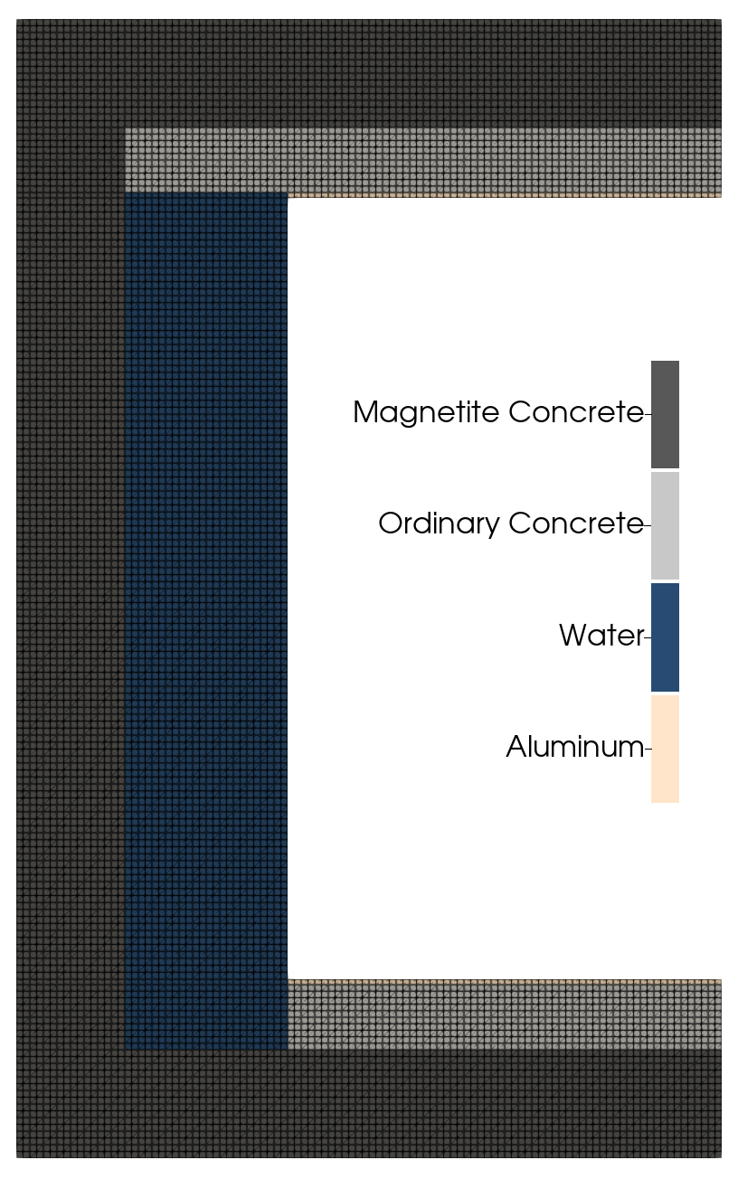
[Mesh]
  [bulk]
    type = CartesianMeshGenerator
    dim = 2
    dx = '0.5 0.75 2.0'
    dy = '0.5 0.3 0.025 3.6 0.025 0.3 0.5'
    ix = '16 24 64'
    iy = '16 10 1 112 1 10 16'
    subdomain_id = '
      0 0 0
      0 2 1
      0 2 3
      0 2 4
      0 2 3
      0 1 1
      0 0 0
    '
  []
  [hollow_concrete]
    type = BlockDeletionGenerator
    input = bulk
    block = 4
  []
  [rename_blocks]
    type = RenameBlockGenerator
    input = hollow_concrete
    old_block = '0 1 2 3'
    new_block = 'concrete_hd concrete water Al'
  []
  [add_concrete_outer_boundary]
    type = RenameBoundaryGenerator
    input = rename_blocks
    old_boundary = 'left right bottom top'
    new_boundary = 'air_boundary symmetry ground air_boundary'
  []
  [add_water_concrete_interface]
    type = SideSetsBetweenSubdomainsGenerator
    input = add_concrete_outer_boundary
    primary_block = 'water water water'
    paired_block = 'concrete_hd concrete Al'
    new_boundary = 'water_boundary'
  []
  [add_water_concrete_interface_inwards]
    type = SideSetsBetweenSubdomainsGenerator
    input = add_water_concrete_interface
    primary_block = 'concrete_hd concrete Al'
    paired_block = 'water water water'
    new_boundary = 'water_boundary_inwards'
  []
  [add_inner_cavity_solid]
    type = SideSetsAroundSubdomainGenerator
    input = add_water_concrete_interface_inwards
    block = Al
    new_boundary = 'inner_cavity_solid'
    include_only_external_sides = true
  []
  [add_inner_cavity_water]
    type = SideSetsAroundSubdomainGenerator
    input = add_inner_cavity_solid
    block = water
    new_boundary = 'inner_cavity_water'
    include_only_external_sides = true
  []
[]
Variable Scaling
To make sure the convergence criterion is fairly applied to all equations, the non-linear variables should be on the same scale.
Making equations non-dimensional is a common technique to achieve this. But this is not typically done in MOOSE, where modelers have direct access to dimensionalized quantities.
MOOSE includes the ability to either manually or automatically scale non-linear variables.
Step 10: Run Input
moose-opt -i mesh2d.i --mesh-only
moose-opt -i step10.i
Step 10: Result
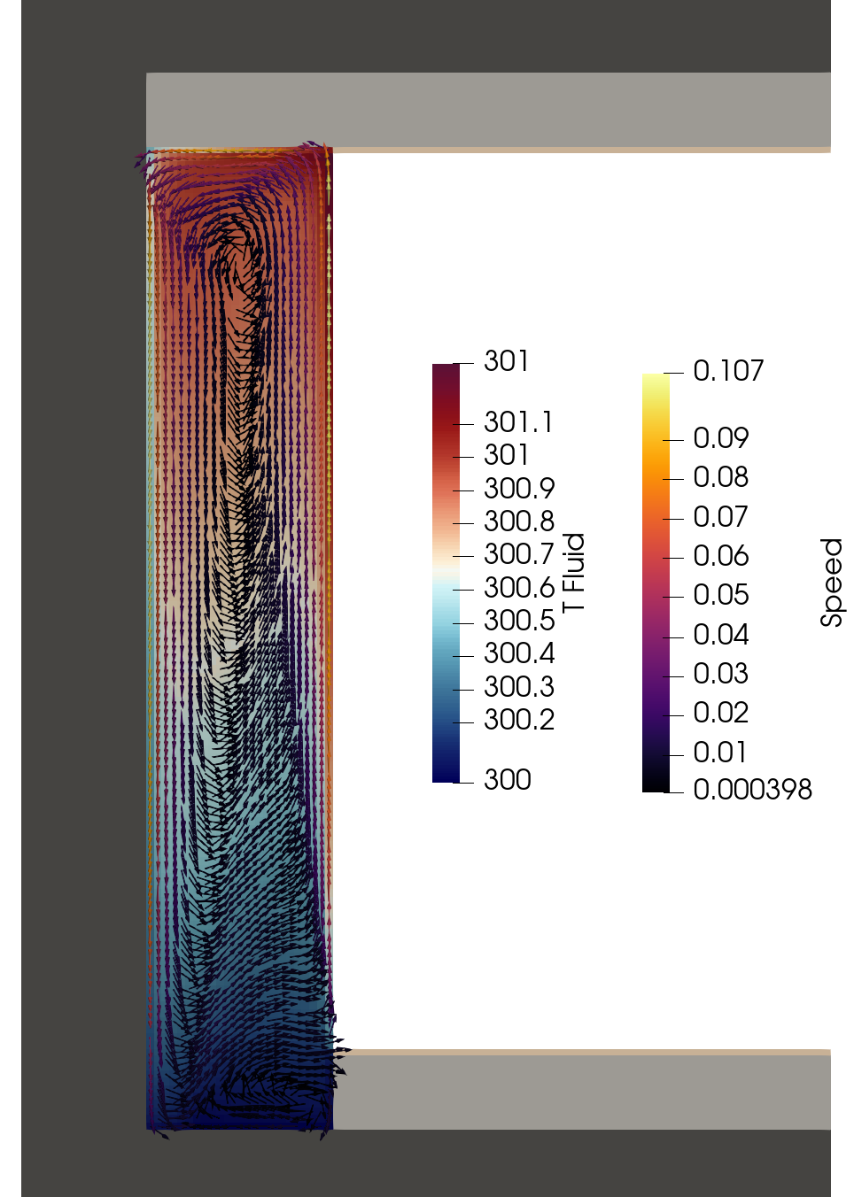
Troubleshooting
Most mistakes in an input file will cause wrong results, usually affecting convergence of the solve as well. We cover here two common problems:
Input file mistakes and how to find them
Non-convergence of the solver
Input file mistakes
If a careful review of the input does not find the error, the next thing to pay attention to is the simulation log.
Are there any warnings? By default MOOSE will not error on warnings
Are there any unused parameters? They could be misspelled!
If that does work, it is time to examine how the simulation evolves in MOOSE
Additional outputs
By default, MOOSE outputs on the end of timesteps
[Outputs]
  execute_on = TIMESTEP_END
We can change this parameter to output as often as linear iterations! We make sure to output material properties as well, in case the problem lies there:
[Outputs]
  [exo]  # filename suffix
    type = Exodus
    execute_on = 'LINEAR TIMESTEP_END'
    output_material_properties = true
  []
[]
Add any output you need to understand the root cause!
Using the Debug system
To look for an issue during setup, we can list the objects created by MOOSE for numerous systems. For example, for material properties,
[Debug]
  show_material_props = true
[]
For a general log on the entire setup:
[Debug]
  show_actions = true
[]
To look for an issue during the execution,
[Debug]
  show_execution_order = ALWAYS
[]
This will output to the console, the execution of all MOOSE's objects, in their respective nodal/elemental/side loops on the mesh.
Troubleshooting failed solves
A comprehensive list of techniques is available in the documentation
First, you should diagnose the non-convergence by printing the residuals for all variables:
[Debug]
  show_var_residual_norms = true
[]
You can then identify which variable is not converging. Equation scaling issues have been covered earlier. Let's explore two other common causes:
initialization
bad mesh
Make sure to initialize every nonlinear variable using the [ICs] block. To check initialization, use the Exodus output:
[Outputs]
  exodus = true
  execute_on = INITIAL
[]
Meshing is hard. We have some tools to help in the MeshGenerator system but generally you should:
visually inspect your mesh. Look for unsupported features: non-conformality (except from libMesh refinement), overlapping cells...
use the MeshDiagnosticsGenerator and turn on the relevant checks
use
show_info = truein the FileMeshGenerator and verify that the output is as expectedreplace your mesh with a simple MOOSE-generated rectangular mesh to check if the mesh is at fault
Summary of helpful resources
Documentation for every object
GitHub discussions forum : please follow the guidelines before posting
Step 11: Multiscale Simulation
We want to
Couple the solid heat conduction solve with the fluid solve and
Study the effects of the local environment on sensors placed in the shield.
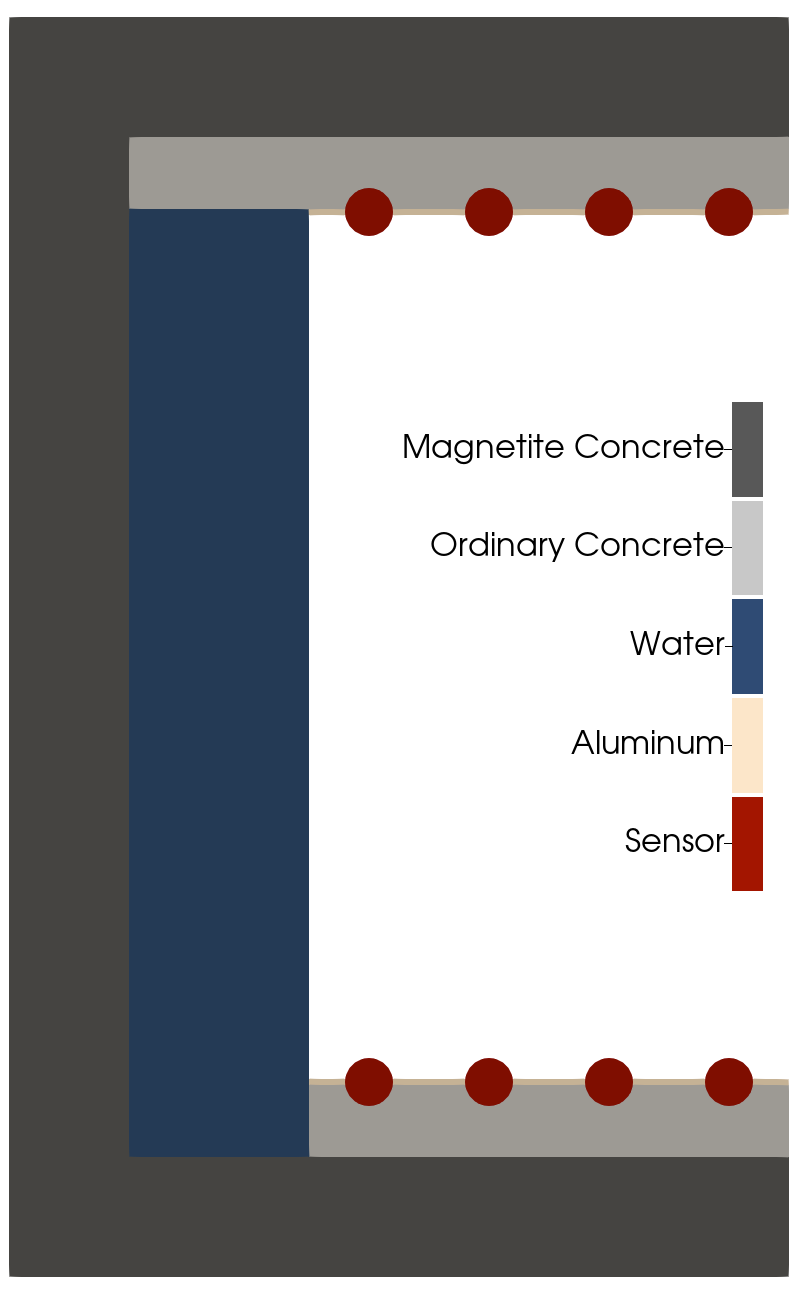
MultiApp System
A system for performing multiple simulations within a main simulation.
MOOSE was originally created to solve fully-coupled systems of PDEs, but not all systems need to be/are fully coupled:
Multiscale systems are generally loosely coupled between scales
Systems with both fast and slow physics can be decoupled in time
Simulations involving input from external codes may be solved
The MultiApp system creates simulations of loosely (or tightly) coupled systems of fully-coupled equations
Coupling terminology
Loosely-Coupled
Each physics solved with a separate linear/nonlinear solve.
Data exchange once per timestep (typically)
Tightly-Coupled / Picard
Each physics solved with a separate linear/nonlinear solve.
Data is exchanged and physics re-solved until “convergence”
Fully-Coupled
All physics solved for in one linear/nonlinear solve

MultiApp Hierarchy
Each "app" is considered to be a solve that is independent, and there is always a "main" that is driving the simulation
The "main" (or "parent") app can have any number of
MultiAppobjectsEach
MultiAppcan represent many sub-applications ("sub-apps" or "child" apps)
Each sub-app can solve for different physics from the main application
A sub-app can be another MOOSE application or could be an external application
A sub-app can have MultiApps, thus create a multi-level solve

Input File Syntax
MultiApp objects are declared in the [MultiApps] block
app_type
The name of the MooseApp derived application to run (e.g., "AnimalApp")
positions
List of 3D coordinates describing the offset of the sub-application into the physical space of the main application
execute_on
Allows control when sub-applications are executed: INITIAL, LINEAR, NONLINEAR, TIMESTEP_BEGIN, TIMESTEP_END
input_files
One input file can be supplied for all the sub-apps or a file can be provided for each
[MultiApps]
  [micro]
    type = TransientMultiApp
    app_type = DarcyThermoMechApp
    positions = '0.01285 0.0    0
                0.01285 0.0608 0
                0.01285 0.1216 0
                0.01285 0.1824 0
                0.01285 0.2432 0
                0.01285 0.304  0'
    input_files = step10_micro.i
    execute_on = 'timestep_end'
  []
[]
Parallel
The MultiApp system is designed for efficient parallel execution of hierarchical problems.
The main application utilizes all processors
The processors are split among each sub-apps within each MultiApp and are run simultaneously
Multiple MultiApps will be executed one after another
Transfer System
A system to move data to and from the "parent application" and "sub-applications" of a MultiApp.
New Feature: Transfers can now send data between sub-applications. We refer to this capability as 'siblings' transfer.
Transferred data typically is received by the Auxiliary and Postprocessor systems.
The data on the receiving application should couple to these values in the normal way and each sub-application should be able to solve on its own.
Field Transfers
Fields can be transferred between applications using a variety of interpolation algorithms.
The direction of the transfer is specified by giving the
from_multi_apporto_multi_appparameter.The source field is evaluated at the destination points (generally nodes or element centroids, depending on the receiving variable type).
The evaluations are then put into the receiving
AuxVariablefield specified by thevariableparameter.GeneralFieldversions of each transfer are implemented using a different algorithm and may be preferred as they support more features.
[Transfers]
  [from_sub]
    source_variable = sub_u
    variable = transferred_u
    type = MultiAppGeneralFieldShapeEvaluationTransfer
    from_multi_app = sub
    execute_on = 'initial timestep_end'
    # Test features non-overlapping meshes
    error_on_miss = false
  []
  [elemental_from_sub]
    source_variable = sub_u
    variable = elemental_transferred_u
    type = MultiAppGeneralFieldShapeEvaluationTransfer
    from_multi_app = sub
    # Test features non-overlapping meshes
    error_on_miss = false
  []
[]
UserObject Interpolation
Many
UserObjectscompute spatially-varying data that is not associated directly with a mesh. For example, local pin-wise averages of a power variable.Any
UserObjectcan overrideReal spatialValue(Point &)to provide a value given a point in spaceA
UserObjectTransfercan sample this spatially-varying data from one app and put the values into anAuxVariablein anotherA
GeneralFieldversions of this transfer is implemented using a different algorithm and may be preferred as it is more feature-complete.
[Transfers]
  [layered_transfer_to_sub_app]
    type = MultiAppUserObjectTransfer
    user_object = main_uo
    variable = sub_app_var
    to_multi_app = sub_app
    displaced_target_mesh = true
  []
  [layered_transfer_from_sub_app]
    type = MultiAppUserObjectTransfer
    user_object = sub_app_uo
    variable = from_sub_app_var
    from_multi_app = sub_app
    displaced_source_mesh = true
  []
[]
Scalar number Transfer
A Postprocessor or a scalar variable transfer allows a transfer of scalar values between applications
When transferring to a
MultiApp, the value can either be put into aPostprocessorvalue or can be put into a constantAuxVariablefield - for example, the main app variable value at the position of the child application can be stored in a postprocessorWhen transferring from a
MultiAppto the parent application, thePostprocessorvalues from all the sub-apps can be interpolated to form an auxiliary field on the parent application
[Transfers]
  [pp_transfer]
    type = MultiAppPostprocessorTransfer
    to_multi_app = pp_sub
    from_postprocessor = average
    to_postprocessor = from_parent
  []
[]
Step 11: Multiscale Simulation
(continued)
Step 11: MultiApp Flow
Three inputs representing each region/physics:
Solid heat conduction:
step11_2d_heat_conduction.iThermal fluids:
step11_2d_fluid.iSensor response:
step11_local.i
Step 11: Fluid Coupling
Fluids Sub-App
Primary difference from the previous step is the addition of the T_solid auxiliary variable, which is used as the "container" for solid heat-conduction app to transfer its solution into.
 @@ -1,26 +1,31 @@
 [AuxVariables]
   # This isn't used in simulation, but useful for visualization
   [vel_z]
     type = INSFVVelocityVariable
     block = 'water'
     initial_condition = 0
   []
   [mixing_length]
     block = 'water'
     order = CONSTANT
     family = MONOMIAL
     fv = true
   []
+  # This is the variable that is transferred from the main app
+  [T_solid]
+    block = 'concrete_hd concrete Al'
+    initial_condition = 300
+  []
 []

 [FVBCs]
   [T_fluid_water_boundary]
     type = FVFunctorConvectiveHeatFluxBC
     boundary = water_boundary
     variable = T_fluid
     T_bulk = T_fluid
-    T_solid = 300
+    T_solid = T_solid
     heat_transfer_coefficient = 600
     is_solid = false
   []
 []
(+ tutorials/shield_multiphysics/inputs/step11_multiapps/step11_2d_fluid.i)
Heat Conduction Main App
[AuxVariables]
  [T_fluid]
    type = INSFVEnergyVariable
    initial_condition = 300
    block = 'water'
  []
[]
[MultiApps]
  [fluid]
    # For pseudo-transient
    type = TransientMultiApp

    # For steady-state fixed-point iteration
    # type = FullSolveMultiApp

    input_files = step11_2d_fluid.i
    execute_on = 'TIMESTEP_END'

    # Pass in parameter values as if from command line
    cli_args = 'power=${power}'
  []
[]

[Transfers]
  [send_T_solid]
    type = MultiAppCopyTransfer
    to_multi_app = fluid
    source_variable = T
    variable = T_solid
  []

  [recv_T_fluid]
    type = MultiAppCopyTransfer
    from_multi_app = fluid
    source_variable = T_fluid
    variable = T_fluid
    to_blocks = 'water'
    from_blocks = 'water'
  []
[]
Multi-Scale Applications
Sensor Sub-App
[Mesh]
  # We make a 3D sphere, but really this could be done in 1D
  [sphere]
    type = SphereMeshGenerator
    radius = 10
    nr = 3
    n_smooth = 10
  []
  # Dimensions of each layer are not realistic
  [HDPE_inner]
    type = ParsedSubdomainMeshGenerator
    input = 'sphere'
    combinatorial_geometry = 'x*x + y*y + z*z < 2*2'
    block_id = 1
  []
  [boron_inner]
    type = ParsedSubdomainMeshGenerator
    input = 'HDPE_inner'
    combinatorial_geometry = '(x*x + y*y + z*z > 2*2) & (x*x + y*y + z*z < 3*3)'
    block_id = 2
  []
  [HDPE_mid]
    type = ParsedSubdomainMeshGenerator
    input = 'boron_inner'
    combinatorial_geometry = '(x*x + y*y + z*z > 3*3) & (x*x + y*y + z*z < 6*6)'
    block_id = 3
  []
  [boron_mid]
    type = ParsedSubdomainMeshGenerator
    input = 'HDPE_mid'
    combinatorial_geometry = '(x*x + y*y + z*z > 6*6) & (x*x + y*y + z*z < 7*7)'
    block_id = 4
  []
  [HDPE_outer]
    type = ParsedSubdomainMeshGenerator
    input = 'boron_mid'
    combinatorial_geometry = 'x*x + y*y + z*z > 7*7'
    block_id = 5
  []
  [rename]
    type = RenameBlockGenerator
    input = 'HDPE_outer'
    old_block = '1 2 3 4 5'
    new_block = 'HDPE_inner boron_inner HDPE_mid boron_mid HDPE_outer'
  []
  [rename_boundary]
    type = RenameBoundaryGenerator
    input = 'rename'
    old_boundary = '0'
    new_boundary = 'outer'
  []

  # length_unit = 0.01
  [scale]
    type = TransformGenerator
    input = rename_boundary
    transform = SCALE
    vector_value = '0.01 0.01 0.01'
  []
[]

[Variables]
  [T]
    initial_condition = 300
  []
[]

# Solve heat equation, with a source from boron absorption
[Kernels]
  [conduction]
    type = HeatConduction
    variable = T
  []
  [source]
    type = CoupledForce
    variable = T
    block = 'boron_inner boron_mid'
    v = flux
    # 2 is our arbitrary value for the group cross section
    coef = 2
  []
[]

[BCs]
  [outer]
    type = PostprocessorDirichletBC
    boundary = 'outer'
    variable = 'T'
    postprocessor = 'T_boundary'
  []
[]

[AuxVariables]
  # Received from the main solve
  [flux]
    initial_condition = 1e5
  []
[]

[Materials]
  [hdpe]
    type = HeatConductionMaterial
    block = 'HDPE_inner HDPE_mid HDPE_outer'
    # arbitrary
    thermal_conductivity = 10
  []
  [boron]
    type = HeatConductionMaterial
    block = 'boron_inner boron_mid'
    # arbitrary
    thermal_conductivity = 7
  []
[]

[Executioner]
  type = Steady
  solve_type = NEWTON
  petsc_options_iname = '-pc_type -pc_hypre_type'
  petsc_options_value = 'hypre boomeramg'
[]

[Postprocessors]
  # Used for boundary condition, received from the main solve
  [T_boundary]
    type = Receiver
    default = 320
  []

  # Compute those then send to the main app
  [T_hdpe_out]
    type = ElementAverageValue
    variable = 'T'
    block = 'HDPE_outer'
  []
  [T_boron_mid]
    type = ElementAverageValue
    variable = 'T'
    block = 'boron_mid'
  []
  [T_hdpe_mid]
    type = ElementAverageValue
    variable = 'T'
    block = 'HDPE_mid'
  []
  [T_boron_inner]
    type = ElementAverageValue
    variable = 'T'
    block = 'boron_inner'
  []
  [T_hdpe_inner]
    type = ElementAverageValue
    variable = 'T'
    block = 'HDPE_inner'
  []
[]

[Outputs]
  exodus = true
[]
Heat Conduction Main App
[AuxVariables]
  [flux]
    [InitialCondition]
      type = FunctionIC
      function = '1e4 * exp(-((x-3.25)^2 + (y-2.225)^2))'
    []
  []

  [T_hdpe_inner]
    family = MONOMIAL
    order = CONSTANT
    block = Al
  []

  [T_boron_inner]
    family = MONOMIAL
    order = CONSTANT
    block = Al
  []
[]

[MultiApps]
  [detectors]
    type = FullSolveMultiApp
    input_files = 'step11_local.i'
    # Create one app at each position
    positions_objects = 'detector_positions'

    # displace the subapp output to their position in the parent app frame
    output_in_position = true

    # compute the global temperature first
    execute_on = 'TIMESTEP_END'

    # Pass in parameter values as if from command line
    cli_args = 'Outputs/console=false'
  []
[]

[Transfers]
  [send_exterior_temperature]
    type = MultiAppVariableValueSamplePostprocessorTransfer
    to_multi_app = detectors
    source_variable = T
    postprocessor = T_boundary
  []

  [send_local_flux]
    type = MultiAppVariableValueSampleTransfer
    to_multi_app = detectors
    source_variable = flux
    variable = flux
  []

  [hdpe_temperature]
    type = MultiAppPostprocessorInterpolationTransfer
    from_multi_app = detectors
    postprocessor = T_hdpe_inner
    variable = T_hdpe_inner
  []

  [boron_temperature]
    type = MultiAppPostprocessorInterpolationTransfer
    from_multi_app = detectors
    postprocessor = T_boron_inner
    variable = T_boron_inner
  []
[]
Step 11: Run Decoupled Physics
Before fully coupled simulation, we must make sure each input file runs well separately.
cd ~/projects/moose/tutorials/shield_multiphysics/inputs/step11_multiapps
moose-opt -i mesh2d_coarse.i --mesh-only
moose-opt -i step11_local.i
moose-opt -i step11_2d_fluid.i
# Disable multiapps and transfers to run the parent application standalone
moose-opt -i step11_2d_heat_conduction.i MultiApps/active='' Transfers/active=''
Sensor temperature field with dummy fixed boundary conditions
Step 11: Run Multi-scale
moose-opt -i step11_2d_heat_conduction.i
The individual sensor results can be plotted 'in-position' in the global geometry.
Postprocessed quantities can be transferred from the local child app meshes to the global mesh.
Step 12: Custom Syntax
Add custom syntax to build objects that are common to all conjugate heat transfer thermal mechanical problems:
Kernels and BCs for solid heat conduction
Objects for solid mechanics
Kernels and BCs for fluid flow
Kernels and BCs for fluid heat transfer
Action System
A system for the programmatic creation of simulation objects and input file syntax.
Syntax
Action recognize syntax such as [Kernels] or [Outputs] and perform actions based on them. Many actions simply create an object, using the type parameter. Other parse parameters in the block and perform the relevant setup steps.
Tasks
The MOOSE action system operates on tasks, each task is connected to one or many actions. Tasks are ordered based on their dependencies, which are set by the developers. This ensures the correctness of the simulation setup. To see tasks being executed, use Debug/show_actions=true.
MooseObjectAction
An action designed to build one or many other MooseObjects, such as in the case of the [Kernels], [Variables], [BCs], etc.. blocks.
Physics
An action designed to build an entire equation. Solid mechanics, computational fluid dynamics, heat conduction are all implemented as Physics. Depending on the Physics, it can include only the kernels, or also include boundary conditions and material properties.
[Physics]
  [SolidMechanics]
    [QuasiStatic]
      [all]
        # This block adds all of the proper Kernels, strain calculators, and Variables
        # for SolidMechanics in the correct coordinate system (autodetected)
        add_variables = true
        strain = FINITE
        eigenstrain_names = eigenstrain
        use_automatic_differentiation = true
        generate_output = 'vonmises_stress elastic_strain_xx elastic_strain_yy strain_xx strain_yy'
      []
    []
  []
[]
Physics are meant to facilitate numerous simulation common needs such as:
multi-system simulation setups
preconditioning
initialization from mesh files
interaction with other
Physics, creating the adequate coupling terms
Step 12: Custom Syntax
(continued)
Step 12: Heat Conduction Physics
Defines the kernels, the boundary conditions of selected supported types, and some numerical parameters
Physics/HeatConduction/FiniteElement
[Physics]
  [HeatConduction]
    [FiniteElement]
      [concrete]
        block = 'concrete_hd concrete Al'
        temperature_name = "T"
        system_names = 'nl0'
        preconditioning = 'defer'

        # Solve for steady state
        # It takes a while to heat up concrete
        initial_temperature = 300
        transient = false

        # Heat conduction boundary conditions can be defined
        # inside the HeatConduction physics block
        fixed_temperature_boundaries = 'ground'
        boundary_temperatures = '300'

        heat_flux_boundaries = 'inner_cavity_solid'
        # 50 kW from radiation, using real surface
        boundary_heat_fluxes = '${power}'

        fixed_convection_boundaries = "water_boundary_inwards air_boundary"
        fixed_convection_T_fluid = "T_fluid 300"
        fixed_convection_htc = "${h_water} 10"
      []
    []
  []
[]
Step 12: Solid Mechanics Physics
Defines the kernels and some helper materials for computing strain.
Physics/SolidMechanics/QuasiStatic
[Physics]
  [SolidMechanics]
    [QuasiStatic]
      [concrete]
        # This block adds all of the proper Kernels, strain calculators, and Variables
        # for Solid Mechanics in the correct coordinate system (autodetected)
        add_variables = true
        strain = FINITE
        eigenstrain_names = eigenstrain
        use_automatic_differentiation = true
        generate_output = 'vonmises_stress elastic_strain_xx elastic_strain_yy strain_xx strain_yy'
        block = 'concrete_hd concrete Al'
      []
    []
  []
[]
Step 12: Fluid Flow Physics
The flow equations are separated from the conservation of energy in the fluid for readability purposes.
Defines both the kernels and the boundary conditions.
[Physics]
  [NavierStokes]
    [Flow]
      [water]
        block = 'water'
        system_names = 'flow'
        compressibility = 'incompressible'

        initial_velocity = '1e-5 1e-5'
        initial_pressure = '1e5'

        # p only appears in a gradient term, and thus could be offset by any constant
        # We pin the pressure to avoid having this nullspace
        pin_pressure = true
        pinned_pressure_type = POINT-VALUE
        pinned_pressure_point = '1 3 0'
        pinned_pressure_value = '1e5'

        gravity = '0 -9.81 0'
        boussinesq_approximation = true
        ref_temperature = 300

        wall_boundaries = 'water_boundary inner_cavity_water'
        momentum_wall_types = 'noslip noslip'
      []
    []
  []
[]
Step 12: Fluid Energy conservation Physics
Physics/NavierStokes/FluidHeatTransfer
[Physics]
  [NavierStokes]
    [FluidHeatTransfer]
      [water]
        block = 'water'
        system_names = 'flow'

        initial_temperature = 300

        # This is a rough coupling to heat conduction
        energy_wall_types = 'convection heatflux'
        energy_wall_functors = 'T:${h_water} ${power}'

        energy_scaling = 1e-5
      []
    []
  []
[]
Step 12: Fluid Turbulence Modeling Physics
Physics/NavierStokes/Turbulence
[Physics]
  [NavierStokes]
    [Turbulence]
      [mixing-length]
        block = 'water'
        turbulence_handling = 'mixing-length'
        coupled_flow_physics = 'water'
        fluid_heat_transfer_physics = 'water'
        system_names = 'flow'
        mixing_length_walls = 'water_boundary inner_cavity_water'
        mixing_length_aux_execute_on = 'initial'
      []
    []
  []
[]
Step 12: Setting up a multi-system simulation
First declare the names of the systems to use in the Problem
[Problem]
  nl_sys_names = 'nl0 flow'
  kernel_coverage_check = false
  material_coverage_check = false
[]
then specify those systems in each Physics.
Step 12: Preconditioning
Multi-system allows for customization of solvers via Preconditioning.
Single Matrix Preconditioner (SMP)
[Preconditioning]
  [thermomecha]
    type = SMP
    nl_sys = 'nl0'
    petsc_options_iname = '-pc_type -pc_hypre_type -ksp_gmres_restart'
    petsc_options_value = 'hypre boomeramg 500'
  []
  [flow]
    type = SMP
    nl_sys = 'flow'
    petsc_options_iname = '-pc_type -pc_factor_shift_type'
    petsc_options_value = 'lu NONZERO'
  []
[]
Step 12: Run
cd ~/projects/moose/tutorials/shield_multiphysics/inputs/step12_physics
moose-opt -i step12.i
Step 12: Results
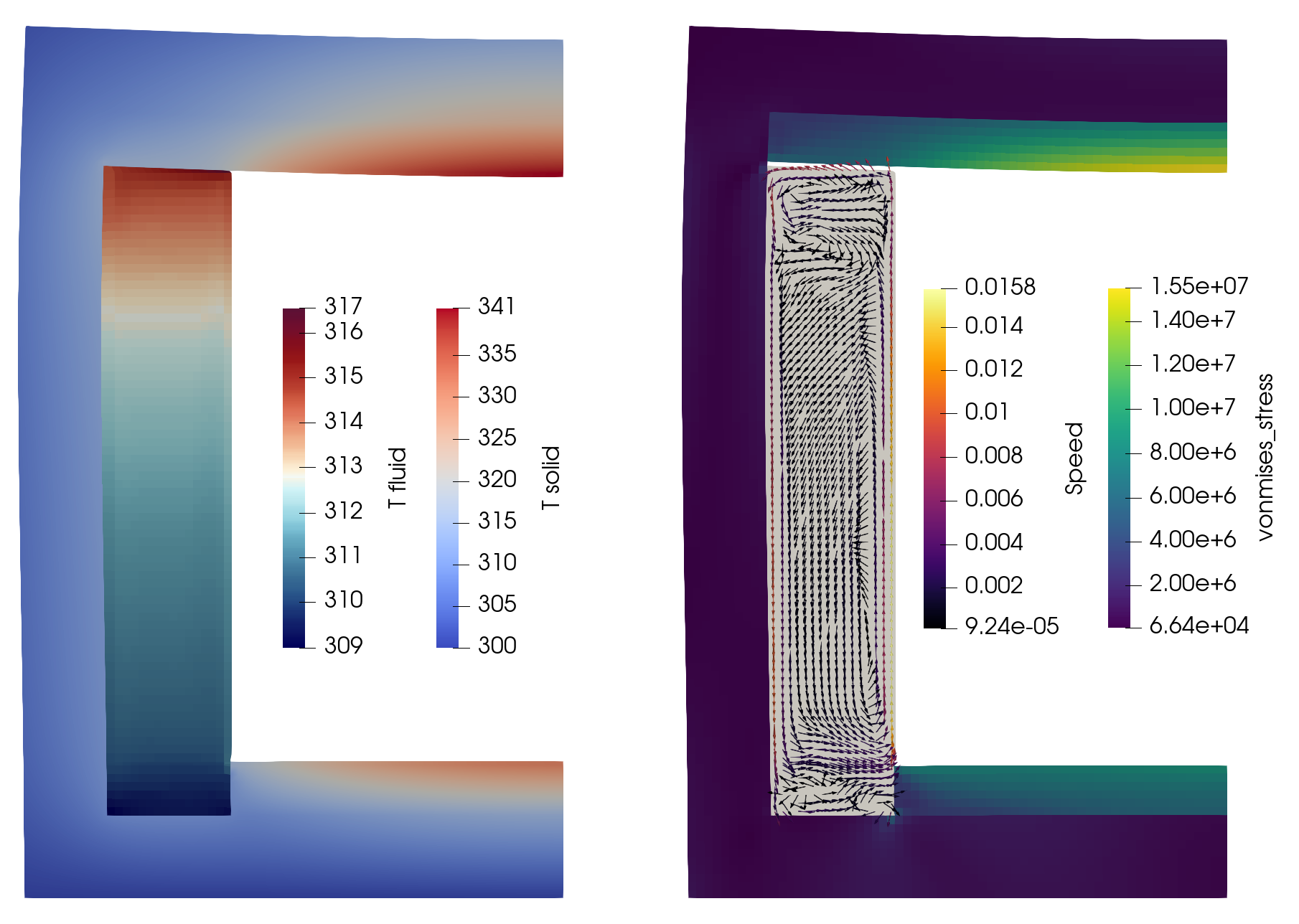
Restart and Recovery System
Definitions
Restart
Running a simulation that uses data from a previous simulation, using different input files
Recover
Resuming an existing simulation after a premature termination
Solution file
A mesh format containing field data in addition to the mesh (i.e. a normal output file)
Checkpoint
A snapshot of the simulation including all meshes, solutions, and stateful data
N to N
In a restart context, this means the number of processors for the previous and current simulations match
N to M
In a restart context, different numbers of processors may be used for the previous and current simulations
Variable Initialization
This method is best suited for restarting a simulation when the mesh in the previous simulation exactly matches the mesh in the current simulation and only initial conditions need to be set for one more variables.
This method requires only a valid solution file
MOOSE supports N to M restart when using this method
Variable Initialization Example
[Mesh]
  # MOOSE supports reading field data from ExodusII, XDA/XDR, and mesh checkpoint files (.e, .xda, .xdr, .cp)
  file = previous.e
  # This method of restart is only supported on serial meshes
  distribution = serial
[]

[Variables/nodal]
  family = LAGRANGE
  order = FIRST
  initial_from_file_var = nodal
  initial_from_file_timestep = 10
[]

[AuxVariables/elemental]
  family = MONOMIAL
  order = CONSTANT
  initial_from_file_var = elemental
  initial_from_file_timestep = 10
[]
Checkpoints
Advanced restart and recovery in MOOSE require checkpoint files
Checkpoints are automatically enabled by default and are output every 1 hour of wall time, but can be disabled with:
[Outputs]
  checkpoint = false
[]
To enable automatic checkpoints using the default options (every time step, and keep last two) in a simulation simply add the following flag to your input file:
[Outputs]
  checkpoint = true
[]
For more control over the checkpoint system, create a sub-block in the input file that will allow you to change the file format, suffix, frequency of output, the number of checkpoint files to keep, etc.
Set
num_filesto at least 2 to minimize the chance of ending up with a corrupt restart file
(test/tests/outputs/checkpoint/checkpoint_interval.i)[Outputs] exodus = true [out] type = Checkpoint time_step_interval = 3 num_files = 2 wall_time_interval = 3600 # seconds [] []
Advanced Restart
This method is best suited for situations when the mesh from the previous simulation and the current simulation match and the variables and stateful data should be loaded from the pervious simulation.
Support for modifying some variables is supported such as
dtandtime_step. By default, MOOSE will automatically use the last values found in the checkpoint filesOnly N to N restarts are supported using this method
[Mesh]
  # Serial number should match corresponding Executioner parameter
  file = out_cp/0010-mesh.cpr
  # This method of restart is only supported on serial meshes
  distribution = serial
[]

[Problem]
  # Note that the suffix is left off in the parameter below.
  restart_file_base = out_cp/LATEST  # You may also use a specific number here
[]
Reloading Data
It is possible to load and project data onto a different mesh from a solution file usually as an initial condition in a new simulation.
MOOSE supports this through the use of a SolutionUserObject
Recover
A simulation that has terminated due to a fault can be recovered simply by using the --recover command-line flag, but it requires a checkpoint file.
./frog-opt -i input.i --recover
Multiapp Restart
When running a multiapp simulation you do not need to enable checkpoint output in each sub app input file. The parent app stores the restart data for all sub apps in its file.
Step 13: Recover, restart and initialization hands-on
Step 13: Recover from Checkpoint
MOOSE can save the exact and entire state of the simulation using a Checkpoint.
[Outputs]
  checkpoint = true
Recover lets us start from the last checkpoint before the simulation stopped.
moose-opt -i step13a_base_calc.i
# Use Ctrl+C / Cmd+C to cancel the calculation
# Recover from the last valid checkpoint
moose-opt -i step13a_base_calc.i --recover
Step 13: Restart from a Checkpoint
[Outputs]
  exodus = true
  checkpoint = true
[]
 @@ -1,13 +1,15 @@
 [Mesh]
   [fmg]
     type = FileMeshGenerator
-    file = '../step03_boundary_conditions/mesh_in.e'
+    file = 'step13a_base_calc_out_cp/LATEST'
   []
 []

 [Problem]
+  # all variables, both nonlinear and auxiliary, are 'restarted'
+  restart_file_base = 'step13a_base_calc_out_cp/LATEST'
   # No kernels on the water domain
   kernel_coverage_check = false
   # No materials on the water domain
   material_coverage_check = false
 []
(+ tutorials/shield_multiphysics/inputs/step13_restart/step13c_restart_from_checkpoint.i)
initial conditions specified in the input override any restarted fields. This must be allowed in the Problem block to avoid unintentional behavior.
moose-opt -i step13a_base_calc.i
moose-opt -i step13c_restart_from_checkpoint.i
Step 13: Initialization from Exodus file
 @@ -1,23 +1,25 @@
 [Mesh]
   [fmg]
     type = FileMeshGenerator
-    file = '../step03_boundary_conditions/mesh_in.e'
+    file = 'step13a_base_calc_out.e'
+    use_for_exodus_restart = true
   []
 []

 [Variables]
   [T]
     # Adds a Linear Lagrange variable by default
     block = 'concrete_hd concrete Al'
-    initial_condition = 300
+    initial_from_file_var = 'T'
   []
 []

 [Executioner]
   type = Transient
-  num_steps = 4
+  start_time = '${units 2 day -> s}'
+  num_steps = 6
   dt = '${units 12 h -> s}'
   solve_type = NEWTON
   petsc_options_iname = '-pc_type -pc_hypre_type'
   petsc_options_value = 'hypre boomeramg'
 []
(+ tutorials/shield_multiphysics/inputs/step13_restart/step13b_initialization_from_exodus.i)
only variables with
initial_from_file_varset will be initializedreading exodus files is a replicated operation, meaning the file is loaded by every process in parallel. Use checkpoint files or a pre-split mesh for parallel mesh reading.
Variables are output to exodus files as linear lagrange or constant monomial, this can create a projection error when restarting.
cd ~/projects/moose/tutorials/shield_multiphysics/inputs/step13_restart
# Generate the initialization file
moose-opt -i step13a_base_calc.i
# Use the exodus file to initialize some variables
moose-opt -i step13b_initialization_from_exodus.i
MOOSE Pluggable Systems
Action System
A system for the programmatic creation of simulation objects and input file syntax.
Auxiliary System
A system for direct calculation of field variables ("AuxVariables") that is designed for postprocessing, coupling, and proxy calculations.
Boundary Condition System
System for computing residual contributions from boundary terms of a PDE.
Constraint System
A system for imposing constraints within a simulation, such as limiting the heat flux across a gap or fixing solution variables across an interface using mortar methods.
Control System
A system for programmatically modifying the input parameters of objects during a simulation.
For example, turning objects on and off:
[Controls]
  [integral_value]
    type = PIDTransientControl
    postprocessor = integral
    target = 1.5
    parameter = 'BCs/left/value'
    K_integral = -1
    K_proportional = -1
    K_derivative = -0.1
    execute_on = 'initial timestep_begin'
  []
[]
Damper System
A system to limit the computed change to the solution during each non-linear iteration to prevent the solver from dramatically changing the solution from one iteration to the next. This may prevent, for example, the solver from attempting to evaluate non-physical values such as negative temperature.
Debug System
A system for debugging a simulation from the input files. It offers several summaries of the objects used, as well as an execution log of Actions and objects during the simulation.
DGKernel System
A system for computing residual contributions for volume terms for the discontinuous Galerkin finite element method.
DiracKernel System
A system for computing residual calculations from point sources.
Distribution System
A system for defining statistical distribution (e.g., uniform, normal, Weibull) functions for use with the stochastic tools module.
Executioner System
A system for dictating the simulation solving strategy.
Executor System
Executors are an experimental system to build composed numerical schemes. Current Executioners can be replaced with their equivalent Executor
Function System
A system for defining analytic expressions based on the spatial location (, , ) and time, .
A Function can depend an other functions, but not on material properties or variables.
Finite Volume Boundary Conditions (FVBCs) System
System for computing residual contributions from boundary terms of a PDE using the finite volume method.
Split between finite volume Dirichlet and flux boundary conditions.
Finite Volume Interface Kernels (FVIKs) System
System for computing residual contributions from interface terms of a PDE using the finite volume method.
The contribution is usually a flux term, identical on both sides of the interface for conservation.
Finite Volume Kernels System
A system for computing the residual contribution of a term within a PDE using the finite volume method.
Finite volume elemental kernels are typically used for volumetric terms (e.g. source, reaction).
Finite volume flux kernels are used for terms integrated by parts (e.g. diffusion) or various fluxes from neighbor cells (e.g. advection).
Geometric Search System
A system for locating geometric elements within a simulation such as the nearest node across a gap.
Initial Condition System
A system for initializing field variables (non-linear and auxiliary) prior to execution of a simulation.
Indicator System
A system for computing an error estimation for use with automatic mesh refinement and coarsening.
InterfaceKernel System
A system to assist in coupling different physics across sub-domains, such as setting the flux of two species to be equivalent across a boundary between two domains.
Kernel System
A system for computing the residual contribution from a volumetric term within a PDE using the Galerkin finite element method.
Line Search System
This system is meant for creating custom line searches for use during the non-linear solve.
Line searches determine the update vector between Newton-Krylov solve iterations.
Marker System
A system for setting status of an element to refine, coarsen, or remain the same for automatic mesh adaptivity.
Material System
A system for defining material properties to be used by multiple systems and allow for variable coupling.
Mesh System
A system for defining a finite element / volume mesh.
Mesh Generator System
A system for generating a finite element mesh using successive geometric construction routines such as building a 2D grid and then extruding into 3D space.
MultiApp System
A system for performing multiple simulations within a main simulation.
Nodal Kernel System
A system for computing a residual contribution of a PDE at nodes within the finite element mesh.
Output System
A system for outputting simulation data to the screen or files.
Parser System
A system for converting input data into MOOSE objects for creating a simulation.
Partitioner System
A system for partitioning a finite element mesh for parallel execution of a simulation.
Positions System
A system for keeping track of the Positions of objects within the mesh during a simulation. It can be leveraged to spawn MultiApps at these locations, to group data near these positions for transfers, and for postprocessing around them.
Postprocessor System
A system for computing a "reduction" or "aggregation" calculation based on the solution variables that results in a single scalar value.
Preconditioner System
A system for defining the preconditioning matrix for use with the non-linear solver.
Predictor System
A system for predicting the next iteration of a simulation based on previous solution iterates.
Problem System
A system for defining the numerical systems that comprise a simulation.
Relationship Manager System
A system for defining geometric or algebraic information needed to perform a calculation in parallel.
This information is then "ghosted", which means it is replicated across all the processes that need it. The information is often ghosted in "layers", for the first few elements near a process' domain boundary.
Reporter System
An advanced system for postprocessing. It is based on a producer/consumer paradigm. Objects may produce reporters, which they declare to the Problem, and other objects may retrieve them from the Problem.
The reporter data can be of very many different types, from a single scalar to maps, vectors and points.
Vectorpostprocessors are an example of reporters, using std::vector<Real> for the reporter data. Reporters include automatic json output.
Sampler System
A system for defining distribution sampling strategies for use with the stochastic tools module.
Split System
A system for splitting the preconditioning matrix to optimize the non-linear solving for multiphysics problems.
Time Integrator System
A system for defining schemes for numerical integration in time.
Time Stepper System
A system for computing time steps for transient executioners.
Transfer System
A system to move data to and from the "parent application" and "sub-applications" of a MultiApp.
New Feature: Transfers can now send data between sub-applications. We refer to this capability as 'siblings' transfer.
UserObject System
A system for defining an arbitrary interface between MOOSE objects.
VectorPostprocessor System
A system for "reduction" or "aggregation" calculations based on the solution variables that results in one or many vectors of values.
References
- Eric B Becker, Graham F Carey, and John Tinsley Oden. Finite Elements, An Introduction: Volume I. Prentice Hall, 6 edition, 1981.
- Jan Flusser, Tomáš Suk, and Barbara Zitová. 2D & 3D image analysis by moments. John Wiley & Sons, Inc., 2016. ISBN 1119039355.
- Luanjing Guo, Hai Huang, Derek R Gaston, Cody J Permann, David Andrs, George D Redden, Chuan Lu, Don T Fox, and Yoshiko Fujita. A parallel, fully coupled, fully implicit solution to reactive transport in porous media using the preconditioned Jacobian-Free Newton-Krylov Method. Advances in Water Resources, 53:101–108, 2013.
- Hrvoje Jasak. Error analysis and estimation for the finite volume method with applications to fluid flows. PhD Thesis, 1996.
- Leslie Kerby, Aaron G Tumulak, Jaakko Leppänen, and Ville Valtavirta. Preliminary Serpent—MOOSE Coupling and Implementation of Functional Expansion Tallies in Serpent. In International Conference on Mathematics & Computational Methods Applied to Nuclear Science and Engineering (M&C 2017). 2017.
- Fadl Moukalled, L Mangani, Marwan Darwish, and others. The finite volume method in computational fluid dynamics. Volume 6. Springer, 2016.
- Brycen Wendt and Leslie Kerby. Multiapp transfers in the moose framework based on functional expansions. Transactions of the American Nuclear Society, 117(1):735–738, October 2017.
- Brycen Wendt, April Novak, Leslie Kerby, and Paul Romano. Integration of functional expansion methodologies as a moose module. In PHYSOR 2018: Reactor Physics paving the way towards more efficient systems. April 2018.