Fracture flow using a MultiApp approach: Porous flow in a simple fracture-matrix system
Background
PorousFlow can be used to simulate flow through fractured porous media in the case when the fracture network is so complicated it cannot be incorporated into the porous-media mesh. The fundamental premise is the fractures can be considered as lower dimensional entities within the higher-dimensional porous media. This page is part of a set that describes a MOOSE MultiApp approach to simulating such models:
MultiApp primer: the diffusion equation with no fractures, and quantifying the errors introduced by the MultiApp approach
Porous flow through a 3D fracture network
A sample PorousFlow simulation through the small 3D fracture network shown in Figure 1 is presented in this section. The methodology is described in the above pages. It is assumed that
the physics is fully-saturated, non-isothermal porous flow with heat conduction and convection;
the porepressure is initially hydrostatic, around 10MPa corresponding to a depth of around 1km;
the temperature is 200C;
injection is into the fracture network only, through one point, at a rate of kg.s and temperature of 100C;
production is from the fracture network only, through one point, at a rate of approximately kg.s (it cannot be exactly kg.s initially because this causes large porepressure reductions due to thermal contraction of water and because the aperture increases in response to the injection);
the fracture aperture dilates elastically in response to enhanced porepressure;
only heat energy is transferred between the fracture and the matrix: the matrix heats the cool water injected into the fracture network.
Figure 1: Fracture network. The injection point is coloured green. The production point is red.
No heat transfer
Before introducing the matrix, consider a model containing just the fracture network.
Physics
The physics is captured by the PorousFlowFullySaturated Action:
[PorousFlowFullySaturated<<<{"href": "../../syntax/PorousFlowFullySaturated/index.html"}>>>]
  coupling_type<<<{"description": "The type of simulation.  For simulations involving Mechanical deformations, you will need to supply the correct Biot coefficient.  For simulations involving Thermal flows, you will need an associated ConstantThermalExpansionCoefficient Material"}>>> = ThermoHydro
  porepressure<<<{"description": "The name of the porepressure variable"}>>> = frac_P
  temperature<<<{"description": "For isothermal simulations, this is the temperature at which fluid properties (and stress-free strains) are evaluated at.  Otherwise, this is the name of the temperature variable.  Units = Kelvin"}>>> = frac_T
  fp<<<{"description": "The name of the user object for fluid properties. Only needed if fluid_properties_type = PorousFlowSingleComponentFluid"}>>> = water
  pressure_unit<<<{"description": "The unit of the pressure variable used everywhere in the input file except for in the FluidProperties-module objects.  This can be set to the non-default value only for fluid_properties_type = PorousFlowSingleComponentFluid"}>>> = MPa
[]Kuzmin-Turek stabilization cannot typically be used for the fracture flow. This is because multiple fracture elements will meet along a single finite-element edge when fracture planes intersect, while for performance reasons, libMesh assumes only one or two elements share an edge. This prevents the KT approach from quantifying flows in all neighboring elements, which prevents the scheme from working.
Because large changes of temperature and pressure are experienced in this model, the Water97 equation of state is employed:
[FluidProperties<<<{"href": "../../syntax/FluidProperties/index.html"}>>>]
  [true_water]
    type = Water97FluidProperties<<<{"description": "Fluid properties for water and steam (H2O) using IAPWS-IF97", "href": "../../source/fluidproperties/Water97FluidProperties.html"}>>>
  []
  [water]
    type = TabulatedBicubicFluidProperties<<<{"description": "Fluid properties using bicubic interpolation on tabulated values provided", "href": "../../source/fluidproperties/TabulatedBicubicFluidProperties.html"}>>>
    fp = true_water
    temperature_min<<<{"description": "Minimum temperature for tabulated data."}>>> = 275 # K
    temperature_max<<<{"description": "Maximum temperature for tabulated data."}>>> = 600
    interpolated_properties<<<{"description": "Properties to interpolate. If unspecified and a data file is provided, the properties from the data file will be used. If specified, some properties from the data file can be ignored."}>>> = 'density viscosity enthalpy internal_energy'
    fluid_property_output_file<<<{"description": "Name of the CSV file which can be output with the tabulation. This file can then be read as a 'fluid_property_file'"}>>> = water97_tabulated.csv
    # Comment out the fp parameter and uncomment below to use the newly generated tabulation
    # fluid_property_file = water97_tabulated.csv
  []
[]Material properties
The insitu fracture aperture is assumed to be mm for all the fracture planes. The fractures are assumed to dilate due to increasing porepressure:
(1)
where m.MPa. Eq. (1) could easily be generalised to include a temperature-dependent term (which would still be modelled using PorousFlowPorosityLinear), or more complicated physics introduced through the use of other PorousFlow porosity classes. Using m.MPa means that a pressure increase of 1MPa dilates the fracture by 1mm.
The page on mathematics and physical interpretation demonstrated that the porosity in the 2D fracture simulation should be multiplied by . Assuming that the porosity of the fracture is 1, the simulation's porosity is :
[Materials<<<{"href": "../../syntax/Materials/index.html"}>>>]
  [porosity]
    type = PorousFlowPorosityLinear<<<{"description": "This Material calculates the porosity in PorousFlow simulations using the relationship porosity_ref + P_coeff * (P - P_ref) + T_coeff * (T - T_ref) + epv_coeff * (epv - epv_ref), where P is the effective porepressure, T is the temperature and epv is the volumetric strain", "href": "../../source/materials/PorousFlowPorosityLinear.html"}>>>
    porosity_ref<<<{"description": "The porosity at reference effective porepressure, temperature and volumetric strain.  This must be a real number or a constant monomial variable (not a linear lagrange or other type of variable)"}>>> = 1E-4 # fracture porosity = 1.0, but must include fracture aperture of 1E-4 at P = insitu_pp
    P_ref<<<{"description": "The reference effective porepressure.  This should usually be a linear-lagrange variable"}>>> = insitu_pp
    P_coeff<<<{"description": "Effective porepressure coefficient"}>>> = 1E-3 # this is in metres/MPa, ie for P_ref = 1/P_coeff, the aperture becomes 1 metre
    porosity_min<<<{"description": "Minimum allowed value of the porosity: if the linear relationship gives values less than this value, then porosity is set to this value instead"}>>> = 1E-5
  []
[]The insitu fracture permeability is assumed to be m. It is assumed that this is , where is a factor capturing the roughness of the fracture surfaces. It is also assumed that when the fracture dilates, this becomes . Because of the multiplication by (see here), the value of permeability used in the simulations is :
(2)
Hence a PorousFlowPermeabilityKozenyCarman Material can be used:
[Materials<<<{"href": "../../syntax/Materials/index.html"}>>>]
  [permeability]
    type = PorousFlowPermeabilityKozenyCarman<<<{"description": "This Material calculates the permeability tensor from a form of the Kozeny-Carman equation based on the spatially constant initial permeability and porosity or grain size.", "href": "../../source/materials/PorousFlowPermeabilityKozenyCarman.html"}>>>
    k0<<<{"description": "The permeability scalar value (usually in m^2) at the reference porosity, required for kozeny_carman_phi0"}>>> = 1E-15 # fracture perm = 1E-11 m^2, but must include fracture aperture of 1E-4
    poroperm_function<<<{"description": "Function relating porosity and permeability. The options are: kozeny_carman_fd2 = f d^2 phi^n/(1-phi)^m (where phi is porosity, f is a scalar constant with typical values 0.01-0.001, and d is grain size). kozeny_carman_phi0 = k0 (1-phi0)^m/phi0^n * phi^n/(1-phi)^m (where phi is porosity, and k0 is the permeability at porosity phi0)  kozeny_carman_A = A for directly supplying the permeability multiplying factor."}>>> = kozeny_carman_phi0
    m<<<{"description": "(1-porosity) exponent"}>>> = 0
    n<<<{"description": "Porosity exponent"}>>> = 3
    phi0<<<{"description": "The reference porosity, required for kozeny_carman_phi0"}>>> = 1E-4
  []
[]PorousFlow's "matrix internal energy" quantifies the internal energy of the rock material. Since there is essentially no rock material within the fracture, the matrix internal energy for the fracture App is zero. It is assumed that the thermal conductivity is constant and independent of (in reality, this too should increase with , but PorousFlow currently lacks this capability, and thermal conductivity is unlikely to be important within the fracture):
[Materials<<<{"href": "../../syntax/Materials/index.html"}>>>]
  [internal_energy]
    type = PorousFlowMatrixInternalEnergy<<<{"description": "This Material calculates the internal energy of solid rock grains, which is specific_heat_capacity * density * temperature.  Kernels multiply this by (1 - porosity) to find the energy density of the porous rock in a rock-fluid system", "href": "../../source/materials/PorousFlowMatrixInternalEnergy.html"}>>>
    density<<<{"description": "Density of the rock grains"}>>> = 2700 # kg/m^3
    specific_heat_capacity<<<{"description": "Specific heat capacity of the rock grains (J/kg/K)."}>>> = 0 # basically no rock inside the fracture
  []
[][Materials<<<{"href": "../../syntax/Materials/index.html"}>>>]
[aq_thermal_conductivity]
type = PorousFlowThermalConductivityIdeal<<<{"description": "This Material calculates rock-fluid combined thermal conductivity by using a weighted sum. Thermal conductivity = dry_thermal_conductivity + S^exponent * (wet_thermal_conductivity - dry_thermal_conductivity), where S is the aqueous saturation", "href": "../../source/materials/PorousFlowThermalConductivityIdeal.html"}>>>
dry_thermal_conductivity<<<{"description": "The thermal conductivity of the rock matrix when the aqueous saturation is zero"}>>> = '0.6E-4 0 0 0 0.6E-4 0 0 0 0.6E-4' # thermal conductivity of water times fracture aperture. This should increase linearly with aperture, but is set constant in this model
[]
[]Injection and production
The Thiem equation may be used to estimate flows to and from the fracture network. Imagine a single well piercing the fracture network in a normal direction to a fracture plane. The Thiem equation is
Here
Q is the flow rate to the well, with SI units kg.s.
is the fluid density: in this case kg.m.
is the fracture permeability: in this case (it is not the 2D version with the "extra" factor of )
is the length of well piercing the fracture network: in this case .
is the change in pressure resulting from the well pumping: .
is the fluid viscosity: in this case MPa.s
is the radius of influence of the well: in this case it is appropriate to choose m since that is the size of the fracture network
is the radius of the borehole. Assume this is m
Eq. (1) may be used to write in terms of . This analysis is only approximate, but it provides a rough idea of the flow rates to expect, as shown in Table 1.
Table 1: Indicative flow rate, aperture and permeability, depending on well pressure
| (MPa) | Q (kg.s) | a (mm) | permeability (m) |
|---|---|---|---|
| 0.1 | 0.004 | 0.2 | |
| 0.2 | 0.03 | 0.3 | |
| 0.5 | 0.5 | 0.6 | |
| 1 | 7 | 1 | |
| 2 | 90 | 2 |
Economically-viable flow rates are usually greater than about 10kg.s, which is the amount prescribed in the MOOSE input file, below. This means a pressure change of MPa is expected, and apertures will be around 1mm. Note that the porepressure around the producer should be around 1MPa higher than insitu, in order for the fluid to flow from the fracture to the production well. If the production well reduces pressure too much, then according to Eq. (1), the fracture will close in its vicinity, resulting in limited fluid production. Therefore, the numerical model relies on the injector increasing the porepressure throughout the system (by greater than 1MPa in most places) and the producer removes excess fluid.
PorousFlow has many different types of sinks and boundary conditions that can be used to model injection and production wells. To most accurately represent the physics around these points, appropriate boundary conditions should be chosen that closely match the operating parameters of the pump infrastructure employed. However, before obsessing over such details, it is worth noting that the fundamental assumption underpinning the PorousFlow module — that the flow is slow — is likely to be violated close to the wells. For instance, if 10kg.s (approximately m.s) is injected into a fracture of aperture 2mm through a borehole of diameter 15cm, the fluid velocity is approximately m.s, which is certainly turbulent and not laminar Darcy flow. This also means that the injection and production pressures predicted by the PorousFlow model are likely to be inaccurate (the true injection pressure is likely to be higher).
For this reason, the current model implements the injection and production rather simply. The injection is implemented using a DirichletBC for the temperature at the injection node:
[BCs<<<{"href": "../../syntax/BCs/index.html"}>>>]
  [inject_heat]
    type = DirichletBC<<<{"description": "Imposes the essential boundary condition $u=g$, where $g$ is a constant, controllable value.", "href": "../../source/bcs/DirichletBC.html"}>>>
    boundary<<<{"description": "The list of boundary IDs from the mesh where this object applies"}>>> = injection_node
    variable<<<{"description": "The name of the variable that this residual object operates on"}>>> = frac_T
    value<<<{"description": "Value of the BC"}>>> = 373
  []
[]and a PorousFlowPointSourceFromPostprocessor DiracKernel for the fluid injection:
[DiracKernels<<<{"href": "../../syntax/DiracKernels/index.html"}>>>]
  [inject_fluid]
    type = PorousFlowPointSourceFromPostprocessor<<<{"description": "Point source (or sink) that adds (or removes) fluid at a mass flux rate specified by a postprocessor.", "href": "../../source/dirackernels/PorousFlowPointSourceFromPostprocessor.html"}>>>
    mass_flux<<<{"description": "The postprocessor name holding the mass flux at this point in kg/s (positive is flux in, negative is flux out)"}>>> = ${injection_rate}
    point<<<{"description": "The x,y,z coordinates of the point source (or sink)"}>>> = '58.8124 0.50384 74.7838'
    variable<<<{"description": "The name of the variable that this residual object operates on"}>>> = frac_P
  []
[]As noted above, the production cannot always be 10kg.s (although it assumes this value at steady-state) so it is implemented using two PorousFlowPeacemanBoreholes: one withdrawing fluid and the other heat energy. There is a minor subtlety that can arise when using PorousFlowPeacemanBoreholes in lower-dimensional input files. Peaceman write the flux as
The prefactor, is automatically included when use_mobility = true, but Peaceman's "well constant", , is
Here is the "3D" permeability, and is the length of borehole that is piercing the fracture system. Hence
is the appropriate lower-dimensional form. This is easily obtained in the MOOSE model by setting line_length = 1 in the input file, and then MOOSE will compute the well constant correctly:
[DiracKernels<<<{"href": "../../syntax/DiracKernels/index.html"}>>>]
  [inject_fluid]
    type = PorousFlowPointSourceFromPostprocessor<<<{"description": "Point source (or sink) that adds (or removes) fluid at a mass flux rate specified by a postprocessor.", "href": "../../source/dirackernels/PorousFlowPointSourceFromPostprocessor.html"}>>>
    mass_flux<<<{"description": "The postprocessor name holding the mass flux at this point in kg/s (positive is flux in, negative is flux out)"}>>> = ${injection_rate}
    point<<<{"description": "The x,y,z coordinates of the point source (or sink)"}>>> = '58.8124 0.50384 74.7838'
    variable<<<{"description": "The name of the variable that this residual object operates on"}>>> = frac_P
  []
  [withdraw_fluid]
    type = PorousFlowPeacemanBorehole<<<{"description": "Approximates a borehole in the mesh using the Peaceman approach, ie using a number of point sinks with given radii whose positions are read from a file.  NOTE: if you are using PorousFlowPorosity that depends on volumetric strain, you should set strain_at_nearest_qp=true in your GlobalParams, to ensure the nodal Porosity Material uses the volumetric strain at the Dirac quadpoints, and can therefore be computed", "href": "../../source/dirackernels/PorousFlowPeacemanBorehole.html"}>>>
    SumQuantityUO<<<{"description": "User Object of type=PorousFlowSumQuantity in which to place the total outflow from the line sink for each time step."}>>> = kg_out_uo
    bottom_p_or_t<<<{"description": "For function_of=pressure, this function is the pressure at the bottom of the borehole, otherwise it is the temperature at the bottom of the borehole."}>>> = 10.6 # 1MPa + approx insitu at production point, to prevent aperture closing due to low porepressures
    character<<<{"description": "If zero then borehole does nothing.  If positive the borehole acts as a sink (production well) for porepressure > borehole pressure, and does nothing otherwise.  If negative the borehole acts as a source (injection well) for porepressure < borehole pressure, and does nothing otherwise.  The flow rate to/from the borehole is multiplied by |character|, so usually character = +/- 1, but you can specify other quantities to provide an overall scaling to the flow if you like."}>>> = 1
    line_length<<<{"description": "Line length.  Note this is only used if there is only one point in the point_file."}>>> = 1
    point_file<<<{"description": "The file containing the coordinates of the points and their weightings that approximate the line sink.  The physical meaning of the weightings depend on the scenario, eg, they may be borehole radii.  Each line in the file must contain a space-separated weight and coordinate, viz r x y z.  For boreholes, the last point in the file is defined as the borehole bottom, where the borehole pressure is bottom_pressure.  If your file contains just one point, you must also specify the line_length and line_direction parameters.  Note that you will get segementation faults if your points do not lie within your mesh!"}>>> = production.xyz
    unit_weight<<<{"description": "(fluid_density*gravitational_acceleration) as a vector pointing downwards.  Note that the borehole pressure at a given z position is bottom_p_or_t + unit_weight*(q - q_bottom), where q=(x,y,z) and q_bottom=(x,y,z) of the bottom point of the borehole.  The analogous formula holds for function_of=temperature.  If you don't want bottomhole pressure (or temperature) to vary in the borehole just set unit_weight=0.  Typical value is = (0,0,-1E4), for water"}>>> = '0 0 0'
    fluid_phase<<<{"description": "The fluid phase whose pressure (and potentially mobility, enthalpy, etc) controls the flux to the line sink.  For p_or_t=temperature, and without any use_*, this parameter is irrelevant"}>>> = 0
    use_mobility<<<{"description": "Multiply the flux by the fluid mobility"}>>> = true
    variable<<<{"description": "The name of the variable that this residual object operates on"}>>> = frac_P
  []
  [withdraw_heat]
    type = PorousFlowPeacemanBorehole<<<{"description": "Approximates a borehole in the mesh using the Peaceman approach, ie using a number of point sinks with given radii whose positions are read from a file.  NOTE: if you are using PorousFlowPorosity that depends on volumetric strain, you should set strain_at_nearest_qp=true in your GlobalParams, to ensure the nodal Porosity Material uses the volumetric strain at the Dirac quadpoints, and can therefore be computed", "href": "../../source/dirackernels/PorousFlowPeacemanBorehole.html"}>>>
    SumQuantityUO<<<{"description": "User Object of type=PorousFlowSumQuantity in which to place the total outflow from the line sink for each time step."}>>> = J_out_uo
    bottom_p_or_t<<<{"description": "For function_of=pressure, this function is the pressure at the bottom of the borehole, otherwise it is the temperature at the bottom of the borehole."}>>> = 10.6 # 1MPa + approx insitu at production point, to prevent aperture closing due to low porepressures
    character<<<{"description": "If zero then borehole does nothing.  If positive the borehole acts as a sink (production well) for porepressure > borehole pressure, and does nothing otherwise.  If negative the borehole acts as a source (injection well) for porepressure < borehole pressure, and does nothing otherwise.  The flow rate to/from the borehole is multiplied by |character|, so usually character = +/- 1, but you can specify other quantities to provide an overall scaling to the flow if you like."}>>> = 1
    line_length<<<{"description": "Line length.  Note this is only used if there is only one point in the point_file."}>>> = 1
    point_file<<<{"description": "The file containing the coordinates of the points and their weightings that approximate the line sink.  The physical meaning of the weightings depend on the scenario, eg, they may be borehole radii.  Each line in the file must contain a space-separated weight and coordinate, viz r x y z.  For boreholes, the last point in the file is defined as the borehole bottom, where the borehole pressure is bottom_pressure.  If your file contains just one point, you must also specify the line_length and line_direction parameters.  Note that you will get segementation faults if your points do not lie within your mesh!"}>>> = production.xyz
    unit_weight<<<{"description": "(fluid_density*gravitational_acceleration) as a vector pointing downwards.  Note that the borehole pressure at a given z position is bottom_p_or_t + unit_weight*(q - q_bottom), where q=(x,y,z) and q_bottom=(x,y,z) of the bottom point of the borehole.  The analogous formula holds for function_of=temperature.  If you don't want bottomhole pressure (or temperature) to vary in the borehole just set unit_weight=0.  Typical value is = (0,0,-1E4), for water"}>>> = '0 0 0'
    fluid_phase<<<{"description": "The fluid phase whose pressure (and potentially mobility, enthalpy, etc) controls the flux to the line sink.  For p_or_t=temperature, and without any use_*, this parameter is irrelevant"}>>> = 0
    use_mobility<<<{"description": "Multiply the flux by the fluid mobility"}>>> = true
    use_enthalpy<<<{"description": "Multiply the flux by the fluid enthalpy"}>>> = true
    variable<<<{"description": "The name of the variable that this residual object operates on"}>>> = frac_T
  []
[]As mentioned above bottom_p_or_t is chosen so that the borehole doesn't "suck" water: instead they rely on the injection to increase the porepressure and pump water into the production borehole. The reason for this is that if the porepressure reduces around the production well (due to a "suck") then the fracture aperture reduces, making it increasingly difficult to extract water.
Results
Typically 3-5 fracture time-steps are taken in a single matrix step in this model. In other models this number could be quite different, but here the fracture and matrix are both approaching steady-state at a similar rate.
The pressure at the injection point rises from its insitu value of around 9.4MPa to around 12.2MPa: an increase of 3MPa, which results in a fracture aperture of around 3mm according to Eq. (1). This results in permeability increasing by a factor of around 27000.
Some results are shown in Figure 2, Figure 3 and Figure 4. Production commences around 1.75 hours after injection starts. These simulations were run using different mesh sizes (by choosing Mesh/uniform_refine appropriately) to illustrate the impact of different meshes in this problem. A straightforward analysis of simulation error as a function of mesh size is not possible, because each simulation also uses a different time-step size. Nevertheless, some observations are:
There is an interesting increase of temperature around the production well in the finer-resolution cases. The reason for this is that a thin layer of insitu hot fluid is "squashed" against the fracture ends as the cold fluid invades the fracture (the thin layer is not resolved in the low-resolution cases). This is also clearly seen in Figure 5. The hot fluid cannot escape, and it becomes pressurized, leading to an increase in temperature. Eventually the porepressure increases to 10.6MPa and the production well activates (indicated by the dot in the figures), withdrawing the hot fluid, and the near-well area cools. In regions where there is no production well, the high temperature eventually diffuses. If the production well were in the middle of a fracture, this interesting phenomenon wouldn't be seen.
As mesh resolution is increased, the results appear to be converging to an "infinite-resolution" case. Given the likely uncertainties in parameter values and the physics of aperture dilation, a mesh with element side-lengths of 10m is likely to be perfectly adequate for this type of problem.
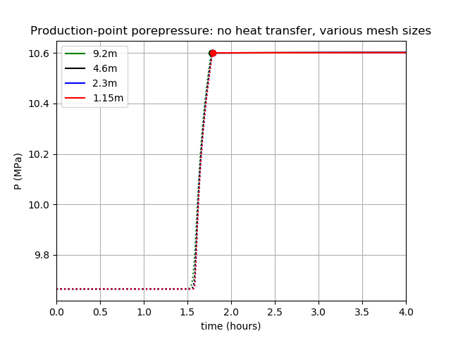
Figure 2: Porepressure at the production point in the case where there is no matrix. The legend's numbers indicate the size of elements used in the simulation. Dotted lines: before production commences. Dot: production commences. Solid lines: during production.
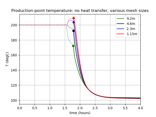
Figure 3: Temperature at the production point in the case where there is no matrix. The legend's numbers indicate the size of elements used in the simulation. Dotted lines: before production commences. Dot: production commences. Solid lines: during production.
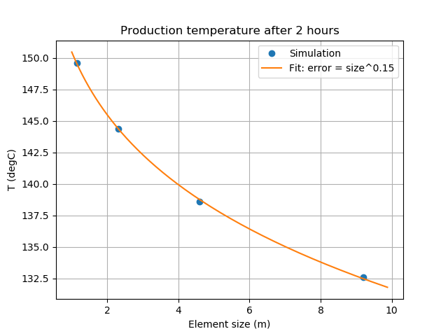
Figure 4: Temperature at the production point 2 hours after injection commences, in the case where there is no matrix, for meshes with different-sized elements. A straightforward error analysis is not possible because each simulation takes different time-steps.
Some animations are shown in Figure 5 and Figure 6. One month is simulated, but steady state is rapidly approached within the first few hours of simulation. The cold injectate invades most of the fracture network: hot pockets of fluid only remain at the tops of some fractures, due to buoyancy.
Figure 5: Temperature in the fracture for the case where there is no matrix, during the first month of simulation. The cold injectate invades most of the fracture network: hot pockets of fluid only remain at the tops of some fractures, due to buoyancy. Time is indicated by the green bar: most of the temperature changes occur within the first few hours
Figure 6: Fracture aperture for the case where there is no matrix, during the first month of simulation. Time is indicated by the green bar: most of the dilation occurs within the first few hours
Including the matrix
Matrix physics and material properties
Most of the matrix input file is standard by now. The physics is governed by PorousFlowFullySaturated
[PorousFlowFullySaturated<<<{"href": "../../syntax/PorousFlowFullySaturated/index.html"}>>>]
  coupling_type<<<{"description": "The type of simulation.  For simulations involving Mechanical deformations, you will need to supply the correct Biot coefficient.  For simulations involving Thermal flows, you will need an associated ConstantThermalExpansionCoefficient Material"}>>> = ThermoHydro
  porepressure<<<{"description": "The name of the porepressure variable"}>>> = matrix_P
  temperature<<<{"description": "For isothermal simulations, this is the temperature at which fluid properties (and stress-free strains) are evaluated at.  Otherwise, this is the name of the temperature variable.  Units = Kelvin"}>>> = matrix_T
  fp<<<{"description": "The name of the user object for fluid properties. Only needed if fluid_properties_type = PorousFlowSingleComponentFluid"}>>> = water
  gravity<<<{"description": "Gravitational acceleration vector downwards (m/s^2)"}>>> = '0 0 -9.81E-6' # Note the value, because of pressure_unit
  pressure_unit<<<{"description": "The unit of the pressure variable used everywhere in the input file except for in the FluidProperties-module objects.  This can be set to the non-default value only for fluid_properties_type = PorousFlowSingleComponentFluid"}>>> = MPa
[]along with the familiar ReporterPointSource:
[DiracKernels<<<{"href": "../../syntax/DiracKernels/index.html"}>>>]
  [heat_from_fracture]
    type = ReporterPointSource<<<{"description": "Apply a point load defined by Reporter.", "href": "../../source/dirackernels/ReporterPointSource.html"}>>>
    variable<<<{"description": "The name of the variable that this residual object operates on"}>>> = matrix_T
    value_name<<<{"description": "reporter value name.  This uses the reporter syntax <reporter>/<name>."}>>> = heat_transfer_rate/transferred_joules_per_s
    x_coord_name<<<{"description": "reporter x-coordinate name.  This uses the reporter syntax <reporter>/<name>."}>>> = heat_transfer_rate/x
    y_coord_name<<<{"description": "reporter y-coordinate name.  This uses the reporter syntax <reporter>/<name>."}>>> = heat_transfer_rate/y
    z_coord_name<<<{"description": "reporter z-coordinate name.  This uses the reporter syntax <reporter>/<name>."}>>> = heat_transfer_rate/z
  []
[]It is assumed the rock matrix has small porosity of 0.1 and permeability of m. The rock density is 2700kg.m with specific heat capacity of 800J.kg.K and isotropic thermal conductivity of 5W.m.K. Hence, the Materials block is:
[Materials<<<{"href": "../../syntax/Materials/index.html"}>>>]
  [porosity]
    type = PorousFlowPorosityConst<<<{"description": "This Material calculates the porosity assuming it is constant", "href": "../../source/materials/PorousFlowPorosityConst.html"}>>>
    porosity<<<{"description": "The porosity (assumed indepenent of porepressure, temperature, strain, etc, for this material).  This should be a real number, or a constant monomial variable (not a linear lagrange or other kind of variable)."}>>> = 1E-3 # small porosity of rock
  []
  [permeability]
    type = PorousFlowPermeabilityConst<<<{"description": "This Material calculates the permeability tensor assuming it is constant", "href": "../../source/materials/PorousFlowPermeabilityConst.html"}>>>
    permeability<<<{"description": "The permeability tensor (usually in m^2), which is assumed constant for this material"}>>> = '1E-18 0 0   0 1E-18 0   0 0 1E-18'
  []
  [internal_energy]
    type = PorousFlowMatrixInternalEnergy<<<{"description": "This Material calculates the internal energy of solid rock grains, which is specific_heat_capacity * density * temperature.  Kernels multiply this by (1 - porosity) to find the energy density of the porous rock in a rock-fluid system", "href": "../../source/materials/PorousFlowMatrixInternalEnergy.html"}>>>
    density<<<{"description": "Density of the rock grains"}>>> = 2700 # kg/m^3
    specific_heat_capacity<<<{"description": "Specific heat capacity of the rock grains (J/kg/K)."}>>> = 800 # rough guess at specific heat capacity
  []
  [aq_thermal_conductivity]
    type = PorousFlowThermalConductivityIdeal<<<{"description": "This Material calculates rock-fluid combined thermal conductivity by using a weighted sum.  Thermal conductivity = dry_thermal_conductivity + S^exponent * (wet_thermal_conductivity - dry_thermal_conductivity), where S is the aqueous saturation", "href": "../../source/materials/PorousFlowThermalConductivityIdeal.html"}>>>
    dry_thermal_conductivity<<<{"description": "The thermal conductivity of the rock matrix when the aqueous saturation is zero"}>>> = '5 0 0  0 5 0  0 0 5'
  []
[]The matrix input file transfers data to the same fracture input file used in the previous section for the fully insulated fracture.
Heat transfer coefficients, matrix mesh sizes and time scales
As mentioned in the mathematical and physical introduction the use of heat transfer coefficients such as
(3)
is only justified if the matrix element sizes are small enough to resolve the physics of interest. (For large elements, not enough heat will be transferred between the fracture and matrix, but the correct short-term behavior could be produced by choosing a larger heat-transfer coefficient than Eq. (3). Naturally, this will result in incorrect long-term behaviour.) The time taken for a pulse of heat to travel through the matrix over half-element distance is
This equation provides a rough idea of the element size needed to accurately resolve physical phenomena. (It also suggests a time-step size: perhaps might be a good choice, but it is likely that the fracture App will need smaller time-steps.) Table 2 enumerates the time-scales for the case in hand: if is smaller than the enumerated time-scale then Eq. (3) is inappropriate, so other choices must be made, or the matrix mesh made finer. (If the matrix mesh is made finer then small time-steps will be needed.)
Table 2: Minimum time-scales for which Eq. (3) will be appropriate, as a function of matrix mesh size
| (m) | matrix mesh size (m) | time scale (days) |
|---|---|---|
| 10 | 20 | 500 |
| 5 | 10 | 125 |
| 2.5 | 5 | 30 |
The heat-transfer is implemented as a PorousFlowHeatMassTransfer Kernel in the fracture input file:
[Kernels<<<{"href": "../../syntax/Kernels/index.html"}>>>]
  [toMatrix]
    type = PorousFlowHeatMassTransfer<<<{"description": "Calculate heat or mass transfer from a coupled variable v to the variable u. No mass lumping is performed here.", "href": "../../source/kernels/PorousFlowHeatMassTransfer.html"}>>>
    variable<<<{"description": "The name of the variable that this residual object operates on"}>>> = frac_T
    v<<<{"description": "The variable which is tranfsered to u using a transfer coefficient"}>>> = transferred_matrix_T
    transfer_coefficient<<<{"description": "Transfer coefficient for heat or mass transferred between variables"}>>> = heat_transfer_coefficient
    save_in<<<{"description": "The name of auxiliary variables to save this Kernel's residual contributions to.  Everything about that variable must match everything about this variable (the type, what blocks it's on, etc.)"}>>> = joules_per_s
  []
[]with being calculated by the following AuxKernel that implements Eq. (3):
[AuxKernels<<<{"href": "../../syntax/AuxKernels/index.html"}>>>]
  [heat_transfer_coefficient_auxk]
    type = ParsedAux<<<{"description": "Sets a field variable value to the evaluation of a parsed expression.", "href": "../../source/auxkernels/ParsedAux.html"}>>>
    variable<<<{"description": "The name of the variable that this object applies to"}>>> = heat_transfer_coefficient
    coupled_variables<<<{"description": "Vector of coupled variable names"}>>> = 'enclosing_element_normal_length enclosing_element_normal_thermal_cond'
    constant_names<<<{"description": "Vector of constants used in the parsed function (use this for kB etc.)"}>>> = h_s
    constant_expressions<<<{"description": "Vector of values for the constants in constant_names (can be an FParser expression)"}>>> = 1E3 # should be much bigger than thermal_conductivity / L ~ 1
    expression<<<{"description": "Parsed function expression to compute"}>>> = 'if(enclosing_element_normal_length = 0, 0, h_s * enclosing_element_normal_thermal_cond * 2 * enclosing_element_normal_length / (h_s * enclosing_element_normal_length * enclosing_element_normal_length + enclosing_element_normal_thermal_cond * 2 * enclosing_element_normal_length))'
  []
[]Coupling and transfers
The simulation's coupling involves the following steps (see also the page on transfers).
Each fracture element must be prescribed with a normal direction, using a ElementNormalAux (formerly
PorousFlowElementNormal) AuxKernel, such as
[AuxKernels<<<{"href": "../../syntax/AuxKernels/index.html"}>>>]
  [normal_dirn_x_auxk]
    type = PorousFlowElementNormal<<<{"description": "AuxKernel to compute components of the element normal.  This is mostly designed for 2D elements living in 3D space, however, the 1D-element and 3D-element cases are handled as special cases.  The Variable for this AuxKernel must be an elemental Variable", "href": "../../source/auxkernels/ElementNormalAux.html"}>>>
    variable<<<{"description": "The name of the variable that this object applies to"}>>> = normal_dirn_x
    component<<<{"description": "The component to compute"}>>> = x
  []
[]Each matrix element must retrieve the fracture-normal information from the nearest fracture element, which is implemented using a MultiAppNearestNodeTransfer Transfer.
[Transfers<<<{"href": "../../syntax/Transfers/index.html"}>>>]
  [normal_x_from_fracture]
    type = MultiAppNearestNodeTransfer<<<{"description": "Transfer the value to the target domain from the nearest node in the source domain.", "href": "../../source/transfers/MultiAppNearestNodeTransfer.html"}>>>
    from_multi_app<<<{"description": "The name of the MultiApp to receive data from"}>>> = fracture_app
    source_variable<<<{"description": "The variable to transfer from."}>>> = normal_dirn_x
    variable<<<{"description": "The auxiliary variable to store the transferred values in."}>>> = fracture_normal_x
  []
[]Each matrix element must be prescribed with a normal length, , using a PorousFlowElementLength AuxKernel and the fracture-normal direction sent to it. As described in the mathematical theory page, this procedure assumes . If then this procedure corresponds to making a shift of the fracture position by an amount less than the finite-element size. Since the accuracy of the finite-element scheme is governed by the element size, such small shifts introduce errors that are smaller than the finite-element error. If a matrix element contains multiple fractures then this procedure only chooses one of their directions. In that case, if the thermal conductivity is anisotropic then the incorrect would be used for all but one of the fractures.
[AuxKernels<<<{"href": "../../syntax/AuxKernels/index.html"}>>>]
  [element_normal_length_auxk]
    type = PorousFlowElementLength<<<{"description": "AuxKernel to compute the 'length' of elements along a given direction.  A plane is constructed through the element's centroid, with normal equal to the direction given.  The average of the distance of the nodal positions to this plane is the 'length' returned.  The Variable for this AuxKernel must be an elemental Variable", "href": "../../source/auxkernels/PorousFlowElementLength.html"}>>>
    variable<<<{"description": "The name of the variable that this object applies to"}>>> = element_normal_length
    direction<<<{"description": "Direction (3-component vector) along which to compute the length.  This may be 3 real numbers, or 3 variables."}>>> = 'fracture_normal_x fracture_normal_y fracture_normal_z'
  []
[]Each matrix element must be prescribed with a normal thermal conductivity, , using the fracture-normal direction, , received from the transfer using , where is the matrix material's anisotropic thermal conductivity tensor. The below input block assumes an isotropic matrix thermal conductivity.
[AuxKernels<<<{"href": "../../syntax/AuxKernels/index.html"}>>>]
  [normal_thermal_conductivity_auxk]
    type = ConstantAux<<<{"description": "Creates a constant field in the domain.", "href": "../../source/auxkernels/ConstantAux.html"}>>>
    variable<<<{"description": "The name of the variable that this object applies to"}>>> = normal_thermal_conductivity
    value<<<{"description": "Some constant value that can be read from the input file"}>>> = 5 # very simple in this case
  []
[]Each fracture element must retrieve and from its nearest matrix element using a MultiAppNearestNodeTransfer, with blocks such as
[Transfers<<<{"href": "../../syntax/Transfers/index.html"}>>>]
  [element_normal_length_to_fracture]
    type = MultiAppNearestNodeTransfer<<<{"description": "Transfer the value to the target domain from the nearest node in the source domain.", "href": "../../source/transfers/MultiAppNearestNodeTransfer.html"}>>>
    to_multi_app<<<{"description": "The name of the MultiApp to transfer the data to"}>>> = fracture_app
    source_variable<<<{"description": "The variable to transfer from."}>>> = element_normal_length
    variable<<<{"description": "The auxiliary variable to store the transferred values in."}>>> = enclosing_element_normal_length
  []
[]Each fracture element must calculate using Eq. (3).
[AuxKernels<<<{"href": "../../syntax/AuxKernels/index.html"}>>>]
  [heat_transfer_coefficient_auxk]
    type = ParsedAux<<<{"description": "Sets a field variable value to the evaluation of a parsed expression.", "href": "../../source/auxkernels/ParsedAux.html"}>>>
    variable<<<{"description": "The name of the variable that this object applies to"}>>> = heat_transfer_coefficient
    coupled_variables<<<{"description": "Vector of coupled variable names"}>>> = 'enclosing_element_normal_length enclosing_element_normal_thermal_cond'
    constant_names<<<{"description": "Vector of constants used in the parsed function (use this for kB etc.)"}>>> = h_s
    constant_expressions<<<{"description": "Vector of values for the constants in constant_names (can be an FParser expression)"}>>> = 1E3 # should be much bigger than thermal_conductivity / L ~ 1
    expression<<<{"description": "Parsed function expression to compute"}>>> = 'if(enclosing_element_normal_length = 0, 0, h_s * enclosing_element_normal_thermal_cond * 2 * enclosing_element_normal_length / (h_s * enclosing_element_normal_length * enclosing_element_normal_length + enclosing_element_normal_thermal_cond * 2 * enclosing_element_normal_length))'
  []
[]These steps could be performed during the simulation initialization, however, it is more convenient to perform them at each time-step. When these steps have been accomplished, each time-step involves the following (which is also used in the sections above).
The matrix temperature,
matrix_T, is sent to the fracture nodes using a MultiAppGeometricInterpolationTransfer Transfer.The fracture physics is solved.
The heat flowing between the fracture and matrix is transferred using a MultiAppReporterTransfer Transfer.
The matrix physics is solved.
The Transfers described above are:
[Transfers<<<{"href": "../../syntax/Transfers/index.html"}>>>]
  [element_normal_length_to_fracture]
    type = MultiAppNearestNodeTransfer<<<{"description": "Transfer the value to the target domain from the nearest node in the source domain.", "href": "../../source/transfers/MultiAppNearestNodeTransfer.html"}>>>
    to_multi_app<<<{"description": "The name of the MultiApp to transfer the data to"}>>> = fracture_app
    source_variable<<<{"description": "The variable to transfer from."}>>> = element_normal_length
    variable<<<{"description": "The auxiliary variable to store the transferred values in."}>>> = enclosing_element_normal_length
  []
  [element_normal_thermal_cond_to_fracture]
    type = MultiAppNearestNodeTransfer<<<{"description": "Transfer the value to the target domain from the nearest node in the source domain.", "href": "../../source/transfers/MultiAppNearestNodeTransfer.html"}>>>
    to_multi_app<<<{"description": "The name of the MultiApp to transfer the data to"}>>> = fracture_app
    source_variable<<<{"description": "The variable to transfer from."}>>> = normal_thermal_conductivity
    variable<<<{"description": "The auxiliary variable to store the transferred values in."}>>> = enclosing_element_normal_thermal_cond
  []
  [T_to_fracture]
    type = MultiAppGeometricInterpolationTransfer<<<{"description": "Transfers the value to the target domain from a combination/interpolation of the values on the nearest nodes in the source domain, using coefficients based on the distance to each node.", "href": "../../source/transfers/MultiAppGeometricInterpolationTransfer.html"}>>>
    to_multi_app<<<{"description": "The name of the MultiApp to transfer the data to"}>>> = fracture_app
    source_variable<<<{"description": "The variable to transfer from."}>>> = matrix_T
    variable<<<{"description": "The auxiliary variable to store the transferred values in."}>>> = transferred_matrix_T
  []
  [normal_x_from_fracture]
    type = MultiAppNearestNodeTransfer<<<{"description": "Transfer the value to the target domain from the nearest node in the source domain.", "href": "../../source/transfers/MultiAppNearestNodeTransfer.html"}>>>
    from_multi_app<<<{"description": "The name of the MultiApp to receive data from"}>>> = fracture_app
    source_variable<<<{"description": "The variable to transfer from."}>>> = normal_dirn_x
    variable<<<{"description": "The auxiliary variable to store the transferred values in."}>>> = fracture_normal_x
  []
  [normal_y_from_fracture]
    type = MultiAppNearestNodeTransfer<<<{"description": "Transfer the value to the target domain from the nearest node in the source domain.", "href": "../../source/transfers/MultiAppNearestNodeTransfer.html"}>>>
    from_multi_app<<<{"description": "The name of the MultiApp to receive data from"}>>> = fracture_app
    source_variable<<<{"description": "The variable to transfer from."}>>> = normal_dirn_y
    variable<<<{"description": "The auxiliary variable to store the transferred values in."}>>> = fracture_normal_y
  []
  [normal_z_from_fracture]
    type = MultiAppNearestNodeTransfer<<<{"description": "Transfer the value to the target domain from the nearest node in the source domain.", "href": "../../source/transfers/MultiAppNearestNodeTransfer.html"}>>>
    from_multi_app<<<{"description": "The name of the MultiApp to receive data from"}>>> = fracture_app
    source_variable<<<{"description": "The variable to transfer from."}>>> = normal_dirn_z
    variable<<<{"description": "The auxiliary variable to store the transferred values in."}>>> = fracture_normal_z
  []
  [heat_from_fracture]
    type = MultiAppReporterTransfer<<<{"description": "Transfers reporter data between two applications.", "href": "../../source/transfers/MultiAppReporterTransfer.html"}>>>
    from_multi_app<<<{"description": "The name of the MultiApp to receive data from"}>>> = fracture_app
    from_reporters<<<{"description": "List of the reporter names (object_name/value_name) to transfer the value from."}>>> = 'heat_transfer_rate/joules_per_s heat_transfer_rate/x heat_transfer_rate/y heat_transfer_rate/z'
    to_reporters<<<{"description": "List of the reporter names (object_name/value_name) to transfer the value to."}>>> = 'heat_transfer_rate/transferred_joules_per_s heat_transfer_rate/x heat_transfer_rate/y heat_transfer_rate/z'
  []
[]Results
Figure 7 and Figure 8 show the temperature at the production bore. It is clear that the matrix provides substantial heat-energy to the injectate, when these results are compared with Figure 3. However, as time proceeds, the cold injectate cools the surrounding matrix, leading to cooler production temperatures. These figures show how the results depend on the matrix and fracture mesh sizes. Keep in mind Table 2, which tabulates the time scale at which the results should become accurate (eg, the "20m, 9.2m" case is not expected to be accurate for time-scales less than about 500 days). Convergence to the infinite-resolution limit is obviously achieved.
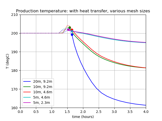
Figure 7: Short-term temperature at the production well. The first number in the legend is the mesh element size, while the second is the fracture element size.
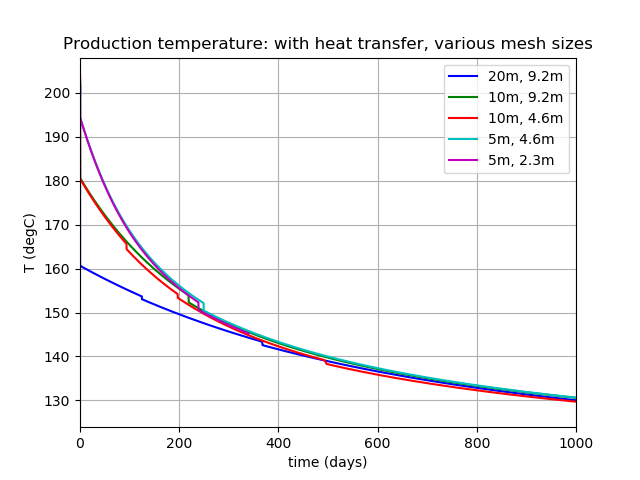
Figure 8: Long-term temperature at the production well. The first number in the legend is the mesh element size, while the second is the fracture element size.
Figure 9 shows the evolution of the cooled matrix material. By 1000 days, an envelope of 10–20m around the fracture system has cooled by more than 10degC. Some parts of the fracture are not cooled at all by the injectate, most particularly those at the top of the network.
Figure 9: Evolution of the cooled matrix material. Colors on the fracture system show fracture temperature. The small boxes are matrix elements that have cooled by more than 10degC. The green color-bar shows the time simulated.
Extensions and comments
This page has described a sample model and workflow for simulating mixed-dimensional, fractured porous systems with PorousFlow. Various simplifying assumptions have been made, and these may need to be modified in a more sophisticated approach.
One of the key assumptions is that fracture aperture is proportional to porepressure change, Eq. (1), and the value of m.MPa was simply chosen to make the results "look reasonable". Ideally, this assumption and value of should be checked experimentally. Alternatively, modellers may implement other well-known equations, which may require a small amount of code development in PorousFlow.
It is likely that the aperture is temperature-dependent, since when the cooled matrix contracts, the fracture will dilate. This effect (if linear) can easily be modelled using PorousFlowPorosityLinear.
No mechanical effects have been included, except via Eq. (1). A different approach would be to treat the matrix as a THM system, transferring the fracture porepressure as an "external" normal stress, , applied in matrix elements containing the fracture. This could be applied as ReporterPointSources. The matrix deforms in response to this as well as changes in matrix temperature. The normal component of the strain, , could be interpreted as an aperture changed, and transferred back to the fracture. This approach contains a few subtleties:
Is matrix strain a good measure of fracture opening?
The matrix element containing the fracture probably needs to be prescribed a modified stiffness, to ensure it adequately models a "fractured element"
Fracture porepressure is a nodal quantity, so for non-planar fractures the normal direction is undefined, so creating an elemental representation of porepressure might be advantageous
Careful consideration of fracture area contained by a matrix element might be advantageous.
Attributing strain in cases where a single matrix element contains multiple fracture elements might be complicated
If fracture elements are huge compared with matrix elements, only the matrix element that happens to contain a fracture node (or element centroid if using elemental porepressure) will experience the additional , while only the matrix element that lies nearest the fracture centroid will provide .
An alternate way of directly including mechanics could be to use the XFEM module and explicitly break matrix elements when they contain fracture elements. The advantage over the previous approach is that it's easy to attribute strain to fracture dilation, but the disadvantage is the complexity of this approach.
Only heat transfer between the fracture and matrix has been considered. Using the methodology outlined in the mathematics page, both fluid transfer and advective heat transfer could be included.
Each fracture has been assumed to have an insitu aperture of 0.1mm. Instead, each fracture could have a unique insitu aperture, and a unique scaling with pressure, by using different material blocks (subdomains).
Fracture porosity has been assumed to be independent of (and hence the 2D version is ), while permeability has been assumed to scale as (hence the 2D version is ). More elaborate versions are certainly possible, but possibly need to be coded into PorousFlow.
The matrix porosity and permeability have been assumed constant and isotropic. Instead, pressure, temperature and strain-dependent versions already coded into PorousFlow could be used.
It is likely that the near-well physics is not accurately captured by PorousFlow, and different physics could be used instead if near-well phenomena and accurate computations of pump pressures are of interest.
Table 2 and the results make it clear that large matrix elements result in "short"-time inaccuracies. It is therefore tempting to refine the matrix mesh around the fracture network. As described in the transfers page, it might be advantageous to use different Transfers if the relative mesh sizes are altered. In the case where matrix elements are smaller than fracture elements, only those few matrix elements that contain fracture nodes will receive heat energy from the fracture system, while only those that lie at the centroid of a fracture element contribute to the aperture calculation.
The injection and production pumps have been modelled in a very simplistic way, and they only act on the fracture system. It would be relatively straightforward to use different pumping strategies.