Fracture flow using a MultiApp approach: Porous flow in a single matrix system
Background
PorousFlow can be used to simulate flow through fractured porous media in the case when the fracture network is so complicated it cannot be incorporated into the porous-media mesh. The fundamental premise is the fractures can be considered as lower dimensional entities within the higher-dimensional porous media. This page is part of a set that describes a MOOSE MultiApp approach to simulating such models:
MultiApp primer: the diffusion equation with no fractures, and quantifying the errors introduced by the MultiApp approach
Porous flow in a single matrix system
Consider a single 1D planar fracture within a 2D mesh. Fluid flows along the fracture according to Darcy's equation, so may be modelled using PorousFlowFullySaturated
[PorousFlowFullySaturated<<<{"href": "../../syntax/PorousFlowFullySaturated/index.html"}>>>]
  coupling_type<<<{"description": "The type of simulation.  For simulations involving Mechanical deformations, you will need to supply the correct Biot coefficient.  For simulations involving Thermal flows, you will need an associated ConstantThermalExpansionCoefficient Material"}>>> = ThermoHydro
  porepressure<<<{"description": "The name of the porepressure variable"}>>> = frac_P
  temperature<<<{"description": "For isothermal simulations, this is the temperature at which fluid properties (and stress-free strains) are evaluated at.  Otherwise, this is the name of the temperature variable.  Units = Kelvin"}>>> = frac_T
  fp<<<{"description": "The name of the user object for fluid properties. Only needed if fluid_properties_type = PorousFlowSingleComponentFluid"}>>> = simple_fluid
  stabilization<<<{"description": "Numerical stabilization used.  'Full' means full upwinding.  'KT' means FEM-TVD stabilization of Kuzmin-Turek"}>>> = KT
  flux_limiter_type<<<{"description": "Type of flux limiter to use if stabilization=KT.  'None' means that no antidiffusion will be added in the Kuzmin-Turek scheme"}>>> = minmod
  gravity<<<{"description": "Gravitational acceleration vector downwards (m/s^2)"}>>> = '0 0 0'
  pressure_unit<<<{"description": "The unit of the pressure variable used everywhere in the input file except for in the FluidProperties-module objects.  This can be set to the non-default value only for fluid_properties_type = PorousFlowSingleComponentFluid"}>>> = MPa
  temperature_unit<<<{"description": "The unit of the temperature variable"}>>> = Celsius
  time_unit<<<{"description": "The unit of time used everywhere in the input file except for in the FluidProperties-module objects.  This can be set to the non-default value only for fluid_properties_type = PorousFlowSingleComponentFluid"}>>> = seconds
[]Kuzmin-Turek stabilization cannot typically be used for the fracture flow. This is because multiple fracture elements will meet along a single finite-element edge when fracture planes intersect, while for performance reasons, libMesh assumes only one or two elements share an edge. This prevents the KT approach from quantifying flows in all neighboring elements, which prevents the scheme from working. In the case at hand, KT stabilization is possible because there is just a single fracture.
The following assumptions are used (see Mathematics and physical interpretation).
The fracture aperture is m, and its porosity is . Therefore, the porosity required by PorousFlow is .
The permeability is given by the formula, modified by a roughness coefficient, , so the permeability required by PorousFlow (which includes the extra factor of ) is .
The fracture is basically filled with water, so the internal energy of any rock material within it may be ignored.
The thermal conductivity in the fracture is dominated by the water (which has thermal conductivity 0.6W.m.K), so the thermal conductivity required by PorousFlow is .
Hence, the Materials are
[Materials<<<{"href": "../../syntax/Materials/index.html"}>>>]
  [porosity]
    type = PorousFlowPorosityConst<<<{"description": "This Material calculates the porosity assuming it is constant", "href": "../../source/materials/PorousFlowPorosityConst.html"}>>>
    porosity<<<{"description": "The porosity (assumed indepenent of porepressure, temperature, strain, etc, for this material).  This should be a real number, or a constant monomial variable (not a linear lagrange or other kind of variable)."}>>> = 1E-2 # includes fracture aperture of 1E-2
  []
  [permeability]
    type = PorousFlowPermeabilityConst<<<{"description": "This Material calculates the permeability tensor assuming it is constant", "href": "../../source/materials/PorousFlowPermeabilityConst.html"}>>>
    permeability<<<{"description": "The permeability tensor (usually in m^2), which is assumed constant for this material"}>>> = '1E-8 0 0   0 1E-8 0   0 0 1E-8' # roughness times a^3/12
  []
  [internal_energy]
    type = PorousFlowMatrixInternalEnergy<<<{"description": "This Material calculates the internal energy of solid rock grains, which is specific_heat_capacity * density * temperature.  Kernels multiply this by (1 - porosity) to find the energy density of the porous rock in a rock-fluid system", "href": "../../source/materials/PorousFlowMatrixInternalEnergy.html"}>>>
    density<<<{"description": "Density of the rock grains"}>>> = 1
    specific_heat_capacity<<<{"description": "Specific heat capacity of the rock grains (J/kg/K)."}>>> = 0 # basically no rock inside the fracture
  []
  [aq_thermal_conductivity]
    type = PorousFlowThermalConductivityIdeal<<<{"description": "This Material calculates rock-fluid combined thermal conductivity by using a weighted sum.  Thermal conductivity = dry_thermal_conductivity + S^exponent * (wet_thermal_conductivity - dry_thermal_conductivity), where S is the aqueous saturation", "href": "../../source/materials/PorousFlowThermalConductivityIdeal.html"}>>>
    dry_thermal_conductivity<<<{"description": "The thermal conductivity of the rock matrix when the aqueous saturation is zero"}>>> = '0.6E-2 0 0  0 0.6E-2 0  0 0 0.6E-2' # thermal conductivity of water times fracture aperture
  []
[]The heat transfer between the fracture and matrix is encoded in the usual way (see the primer and the diffusion pages). The heat transfer coefficient is chosen to be 100, just so that an appreciable amount of heat energy is transferred, not because this is a realistic transfer coefficient for this case:
[Kernels<<<{"href": "../../syntax/Kernels/index.html"}>>>]
  [toMatrix]
    type = PorousFlowHeatMassTransfer<<<{"description": "Calculate heat or mass transfer from a coupled variable v to the variable u. No mass lumping is performed here.", "href": "../../source/kernels/PorousFlowHeatMassTransfer.html"}>>>
    variable<<<{"description": "The name of the variable that this residual object operates on"}>>> = frac_T
    v<<<{"description": "The variable which is tranfsered to u using a transfer coefficient"}>>> = transferred_matrix_T
    transfer_coefficient<<<{"description": "Transfer coefficient for heat or mass transferred between variables"}>>> = 1E2
    save_in<<<{"description": "The name of auxiliary variables to save this Kernel's residual contributions to.  Everything about that variable must match everything about this variable (the type, what blocks it's on, etc.)"}>>> = joules_per_s
  []
[]The boundary conditions correspond to injection of 100C water at a rate of 10kg.s at the left side of the model, and withdrawal of water at the same rate (and whatever temperature it is extracted at) at the right side:
      [left_injection]
        type = PorousFlowSinkBC
        boundary = left
        fluid_phase = 0
        T_in = 373 # Kelvin!
        fp = simple_fluid
        flux_function = -10 # 10 kg/s
[BCs<<<{"href": "../../syntax/BCs/index.html"}>>>]
  [mass_production]
    type = PorousFlowSink<<<{"description": "Applies a flux sink to a boundary.", "href": "../../source/bcs/PorousFlowSink.html"}>>>
    boundary<<<{"description": "The list of boundary IDs from the mesh where this object applies"}>>> = right
    variable<<<{"description": "The name of the variable that this residual object operates on"}>>> = frac_P
    flux_function<<<{"description": "The flux.  The flux is OUT of the medium: hence positive values of this function means this BC will act as a SINK, while negative values indicate this flux will be a SOURCE.  The functional form is useful for spatially or temporally varying sinks.  Without any use_*, this function is measured in kg.m^-2.s^-1 (or J.m^-2.s^-1 for the case with only heat and no fluids)"}>>> = 10
  []
  [heat_production]
    type = PorousFlowSink<<<{"description": "Applies a flux sink to a boundary.", "href": "../../source/bcs/PorousFlowSink.html"}>>>
    boundary<<<{"description": "The list of boundary IDs from the mesh where this object applies"}>>> = right
    variable<<<{"description": "The name of the variable that this residual object operates on"}>>> = frac_T
    flux_function<<<{"description": "The flux.  The flux is OUT of the medium: hence positive values of this function means this BC will act as a SINK, while negative values indicate this flux will be a SOURCE.  The functional form is useful for spatially or temporally varying sinks.  Without any use_*, this function is measured in kg.m^-2.s^-1 (or J.m^-2.s^-1 for the case with only heat and no fluids)"}>>> = 10
    fluid_phase<<<{"description": "If supplied, then this BC will potentially be a function of fluid pressure, and you can use mass_fraction_component, use_mobility, use_relperm, use_enthalpy and use_energy.  If not supplied, then this BC can only be a function of temperature"}>>> = 0
    use_enthalpy<<<{"description": "If true, then fluxes are multiplied by enthalpy.  In this case bare_flux is measured in kg.m^-2.s^-1 / (J.kg).  This can be used in conjunction with other use_*"}>>> = true
  []
[]The physics in the matrix is assumed to be the simple heat equation. Note that this has no stabilization, so there are overshoots and undershoots in the solution.
[Kernels<<<{"href": "../../syntax/Kernels/index.html"}>>>]
  [dot]
    type = CoefTimeDerivative<<<{"description": "The time derivative operator with the weak form of $(\\psi_i, \\frac{\\partial u_h}{\\partial t})$.", "href": "../../source/kernels/CoefTimeDerivative.html"}>>>
    variable<<<{"description": "The name of the variable that this residual object operates on"}>>> = matrix_T
    Coefficient<<<{"description": "The coefficient for the time derivative kernel"}>>> = 1E5
  []
  [matrix_diffusion]
    type = AnisotropicDiffusion<<<{"description": "Anisotropic diffusion kernel $\\nabla \\cdot -\\widetilde{k} \\nabla u$ with weak form given by $(\\nabla \\psi_i, \\widetilde{k} \\nabla u)$.", "href": "../../source/kernels/AnisotropicDiffusion.html"}>>>
    variable<<<{"description": "The name of the variable that this residual object operates on"}>>> = matrix_T
    tensor_coeff<<<{"description": "The Tensor to multiply the Diffusion operator by"}>>> = '1 0 0 0 1 0 0 0 1'
  []
[]The Transfers are identical to those used in the diffusion-equation case:
[Transfers<<<{"href": "../../syntax/Transfers/index.html"}>>>]
  [T_to_fracture]
    type = MultiAppGeometricInterpolationTransfer<<<{"description": "Transfers the value to the target domain from a combination/interpolation of the values on the nearest nodes in the source domain, using coefficients based on the distance to each node.", "href": "../../source/transfers/MultiAppGeometricInterpolationTransfer.html"}>>>
    to_multi_app<<<{"description": "The name of the MultiApp to transfer the data to"}>>> = fracture_app
    source_variable<<<{"description": "The variable to transfer from."}>>> = matrix_T
    variable<<<{"description": "The auxiliary variable to store the transferred values in."}>>> = transferred_matrix_T
  []
  [heat_from_fracture]
    type = MultiAppReporterTransfer<<<{"description": "Transfers reporter data between two applications.", "href": "../../source/transfers/MultiAppReporterTransfer.html"}>>>
    from_multi_app<<<{"description": "The name of the MultiApp to receive data from"}>>> = fracture_app
    from_reporters<<<{"description": "List of the reporter names (object_name/value_name) to transfer the value from."}>>> = 'heat_transfer_rate/joules_per_s heat_transfer_rate/x heat_transfer_rate/y heat_transfer_rate/z'
    to_reporters<<<{"description": "List of the reporter names (object_name/value_name) to transfer the value to."}>>> = 'heat_transfer_rate/transferred_joules_per_s heat_transfer_rate/x heat_transfer_rate/y heat_transfer_rate/z'
  []
[]The fracture-matrix-fracture-matrix-etc time-stepping procedure is the same as described in the primer. Remember that the MultiApp approach typically breaks the unconditional stability of MOOSE's implicit time-stepping scheme. This is because usually the fracture physics is "frozen" while the matrix physics is evolving, and vice-versa. This can easily lead to oscillations if the time-step is too big. For example, start with a cold matrix and hot fracture. When the fracture evolves, it could transfer a huge amount of heat energy to the cold matrix, since the matrix temperature is fixed. During its evolution, the matrix starts hot, so transfers the heat back to the fracture. This cycle continues.
After 100s of simulation, the matrix temperature is shown in Figure 1. The evolution of the temperatures is shown in Figure 2. Without any heat transfer, the fracture heats up to 100C, but when the fracture transfers heat energy to the matrix, the temperature evolution is retarded.
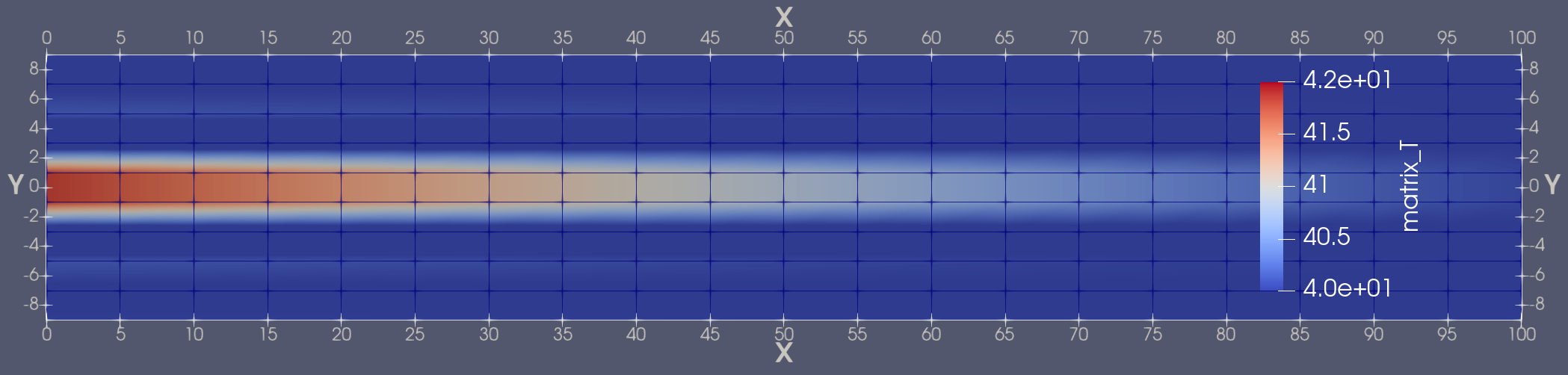
Figure 1: Heat conduction into the matrix (the matrix mesh is shown)
Figure 2: Temperature along the fracture, with heat transfer to the matrix and without heat transfer to the matrix. Fluid at 100degC is injected into the fracture at its left end, and fluid is withdrawn at the right end. With heat transfer, the matrix heats up a little.