Point and line sources/sinks
A number of sources/sinks are available in Porous Flow, implemented as DiracKernels. This page may be read in conjunction with the description of some Dirac Kernel tests. Descriptions of tests of point sources and sinks in multi-phase, multi-component scenarios may be found here.
Constant point source
PorousFlowSquarePulsePointSource implements a constant mass point source that adds (removes) fluid at a constant mass flux rate (kg.s) for times between the specified start and end times. If no start and end times are specified, the source (sink) starts at the start of the simulation and continues to act indefinitely. For instance:
[DiracKernels<<<{"href": "../../syntax/DiracKernels/index.html"}>>>]
  [sink1]
    type = PorousFlowSquarePulsePointSource<<<{"description": "Point source (or sink) that adds (removes) fluid at a constant mass flux rate for times between the specified start and end times.", "href": "../../source/dirackernels/PorousFlowSquarePulsePointSource.html"}>>>
    start_time<<<{"description": "The time at which the source will start (Default is 0)"}>>> = 100
    end_time<<<{"description": "The time at which the source will end (Default is 1e30)"}>>> = 300
    point<<<{"description": "The x,y,z coordinates of the point source (sink)"}>>> = '0.5 0.5 0'
    mass_flux<<<{"description": "The mass flux at this point in kg/s (positive is flux in, negative is flux out)"}>>> = -0.1
    variable<<<{"description": "The name of the variable that this residual object operates on"}>>> = pp
  []
  [sink]
    type = PorousFlowSquarePulsePointSource<<<{"description": "Point source (or sink) that adds (removes) fluid at a constant mass flux rate for times between the specified start and end times.", "href": "../../source/dirackernels/PorousFlowSquarePulsePointSource.html"}>>>
    start_time<<<{"description": "The time at which the source will start (Default is 0)"}>>> = 600
    end_time<<<{"description": "The time at which the source will end (Default is 1e30)"}>>> = 1400
    point<<<{"description": "The x,y,z coordinates of the point source (sink)"}>>> = '0.5 0.5 0'
    mass_flux<<<{"description": "The mass flux at this point in kg/s (positive is flux in, negative is flux out)"}>>> = -0.1
    variable<<<{"description": "The name of the variable that this residual object operates on"}>>> = pp
  []
  [source]
    point<<<{"description": "The x,y,z coordinates of the point source (sink)"}>>> = '0.5 0.5 0'
    start_time<<<{"description": "The time at which the source will start (Default is 0)"}>>> = 1500
    mass_flux<<<{"description": "The mass flux at this point in kg/s (positive is flux in, negative is flux out)"}>>> = 0.2
    end_time<<<{"description": "The time at which the source will end (Default is 1e30)"}>>> = 2000
    variable<<<{"description": "The name of the variable that this residual object operates on"}>>> = pp
    type = PorousFlowSquarePulsePointSource<<<{"description": "Point source (or sink) that adds (removes) fluid at a constant mass flux rate for times between the specified start and end times.", "href": "../../source/dirackernels/PorousFlowSquarePulsePointSource.html"}>>>
  []
[]Note that the parameter mass_flux is positive for a source and negative for a sink, which is dissimilar to the conventions used below for line-sink strength and flux .
Point source from postprocessor
A mass point source can be specified via a value computed by a postprocessor using PorousFlowPointSourceFromPostprocessor Dirac kernel. Users have to make sure that the postprocessor is evaluated at timestep_begin so that the correct value is used within the timestep.
Such example is shown here:
[DiracKernels<<<{"href": "../../syntax/DiracKernels/index.html"}>>>]
  [source]
    type = PorousFlowPointSourceFromPostprocessor<<<{"description": "Point source (or sink) that adds (or removes) fluid at a mass flux rate specified by a postprocessor.", "href": "../../source/dirackernels/PorousFlowPointSourceFromPostprocessor.html"}>>>
    variable<<<{"description": "The name of the variable that this residual object operates on"}>>> = pp
    mass_flux<<<{"description": "The postprocessor name holding the mass flux at this point in kg/s (positive is flux in, negative is flux out)"}>>> = mass_flux_in
    point<<<{"description": "The x,y,z coordinates of the point source (or sink)"}>>> = '0.5 0.5 0'
  []
[][Postprocessors<<<{"href": "../../syntax/Postprocessors/index.html"}>>>]
[total_mass]
type = PorousFlowFluidMass<<<{"description": "Calculates the mass of a fluid component in a region", "href": "../../source/postprocessors/PorousFlowFluidMass.html"}>>>
execute_on<<<{"description": "The list of flag(s) indicating when this object should be executed. For a description of each flag, see https://mooseframework.inl.gov/source/interfaces/SetupInterface.html."}>>> = 'initial timestep_end'
[]
[mass_flux_in]
type = FunctionValuePostprocessor<<<{"description": "Computes the value of a supplied function at a single point (scalable)", "href": "../../source/postprocessors/FunctionValuePostprocessor.html"}>>>
function<<<{"description": "The function which supplies the postprocessor value."}>>> = mass_flux_fn
execute_on<<<{"description": "The list of flag(s) indicating when this object should be executed. For a description of each flag, see https://mooseframework.inl.gov/source/interfaces/SetupInterface.html."}>>> = 'initial timestep_begin'
[]
[]Note that the parameter mass_flux is positive for a source and negative for a sink.
Injecting fluid at specified temperature
When injecting a fluid at specified temperature (also computed as a postprocessor), users can add another Dirac kernel PorousFlowPointEnthalpySourceFromPostprocessor. (Alternately, users can also fix the temperature of an injected fluid using a Dirichlet BC, but this adds/subtracts heat energy to entire nodal volumes of porous material and fluid, so may lead to unacceptable errors from the additional heat energies added/removed.)
Such example is shown here:
[DiracKernels<<<{"href": "../../syntax/DiracKernels/index.html"}>>>]
  [source]
    type = PorousFlowPointSourceFromPostprocessor<<<{"description": "Point source (or sink) that adds (or removes) fluid at a mass flux rate specified by a postprocessor.", "href": "../../source/dirackernels/PorousFlowPointSourceFromPostprocessor.html"}>>>
    variable<<<{"description": "The name of the variable that this residual object operates on"}>>> = pressure
    mass_flux<<<{"description": "The postprocessor name holding the mass flux at this point in kg/s (positive is flux in, negative is flux out)"}>>> = mass_flux_in
    point<<<{"description": "The x,y,z coordinates of the point source (or sink)"}>>> = '0.5 0.5 0'
  []
  [source_h]
    type = PorousFlowPointEnthalpySourceFromPostprocessor<<<{"description": "Point source that adds heat energy corresponding to injection of a fluid with specified mass flux rate (specified by a postprocessor) at given temperature (specified by a postprocessor)", "href": "../../source/dirackernels/PorousFlowPointEnthalpySourceFromPostprocessor.html"}>>>
    variable<<<{"description": "The name of the variable that this residual object operates on"}>>> = temperature
    mass_flux<<<{"description": "The postprocessor name holding the mass flux of injected fluid at this point in kg/s (please ensure this is positive so that this object acts like a source)"}>>> = mass_flux_in
    point<<<{"description": "The x,y,z coordinates of the point source"}>>> = '0.5 0.5 0'
    T_in<<<{"description": "The postprocessor name holding the temperature of injected fluid (measured in K)"}>>> = T_in
    pressure<<<{"description": "Pressure used to calculate the injected fluid enthalpy (measured in Pa)"}>>> = pressure
    fp<<<{"description": "The name of the user object used to calculate the fluid properties of the injected fluid"}>>> = simple_fluid
  []
[][Postprocessors<<<{"href": "../../syntax/Postprocessors/index.html"}>>>]
[total_mass]
type = PorousFlowFluidMass<<<{"description": "Calculates the mass of a fluid component in a region", "href": "../../source/postprocessors/PorousFlowFluidMass.html"}>>>
execute_on<<<{"description": "The list of flag(s) indicating when this object should be executed. For a description of each flag, see https://mooseframework.inl.gov/source/interfaces/SetupInterface.html."}>>> = 'initial timestep_end'
[]
[total_heat]
type = PorousFlowHeatEnergy<<<{"description": "Calculates the sum of heat energy of fluid phase(s) and/or the porous skeleton in a region", "href": "../../source/postprocessors/PorousFlowHeatEnergy.html"}>>>
[]
[mass_flux_in]
type = FunctionValuePostprocessor<<<{"description": "Computes the value of a supplied function at a single point (scalable)", "href": "../../source/postprocessors/FunctionValuePostprocessor.html"}>>>
function<<<{"description": "The function which supplies the postprocessor value."}>>> = mass_flux_in_fn
execute_on<<<{"description": "The list of flag(s) indicating when this object should be executed. For a description of each flag, see https://mooseframework.inl.gov/source/interfaces/SetupInterface.html."}>>> = 'initial timestep_end'
[]
[avg_temp]
type = ElementAverageValue<<<{"description": "Computes the volumetric average of a variable", "href": "../../source/postprocessors/ElementAverageValue.html"}>>>
variable<<<{"description": "The name of the variable that this object operates on"}>>> = temperature
execute_on<<<{"description": "The list of flag(s) indicating when this object should be executed. For a description of each flag, see https://mooseframework.inl.gov/source/interfaces/SetupInterface.html."}>>> = 'initial timestep_end'
[]
[T_in]
type = FunctionValuePostprocessor<<<{"description": "Computes the value of a supplied function at a single point (scalable)", "href": "../../source/postprocessors/FunctionValuePostprocessor.html"}>>>
function<<<{"description": "The function which supplies the postprocessor value."}>>> = T_in_fn
execute_on<<<{"description": "The list of flag(s) indicating when this object should be executed. For a description of each flag, see https://mooseframework.inl.gov/source/interfaces/SetupInterface.html."}>>> = 'initial timestep_end'
[]
[]PorousFlow polyline sinks in general
Two types of polyline sinks are implemented in PorousFlow: the PorousFlowPolyLineSink and the PorousFlowPeacemanBorehole. These are extensions and specialisations of the general PorousFlowLineSink (that is not available to use in an input file) which is described in this section.
Polyline sinks and sources are modelled as sequences of discrete points: The sink is (1) Here is a volume source, measured in kg.m.s (or J.m.s for heat flow), which when integrated over the finite element yields just the "sink strength", , which has units kg.s for fluid flow, or J.s for heat flow. The sink strength is the parameter that is specified by the user in the input file, and the parameters are convenient weights that are discussed below.
The strength, , is a function of porepressure and/or temperature, and may involve other quantities, as enumerated below. The convention followed is:
A sink has . This removes fluid or heat from the simulation domain;
A source has . This adds fluid or heat to the simulation domain.
There are two separate input formats for the PorousFlow polyline sink. The first requires the location for each point along the line length to be specified. The second is relevant for straight lines only, and requires a starting location, direction and length.
The first input format can be defined by either a plain text file or a reporter. In the plain text file, each point is specified by a line containing the following space-separated quantities: (2)
The weighting terms, , are for user convenience, but for the Peaceman borehole case they are the borehole radius at point .
The reporter format for point data supplies the same coordinate and weighting data using the following syntax:
    weight_reporter='pls02file/w'
    x_coord_reporter='pls02file/x'
    y_coord_reporter='pls02file/y'
z_coord_reporter='pls02file/z'where the polyline coordinates and weighting are defined in the following ConstantReporter:
[Reporters<<<{"href": "../../syntax/Reporters/index.html"}>>>]
  [pls02file]
    # contains contents from pls02.bh
    type = ConstantReporter<<<{"description": "Reporter with constant values to be accessed by other objects, can be modified using transfers.", "href": "../../source/reporters/ConstantReporter.html"}>>>
    real_vector_names<<<{"description": "Names for each vector of reals value."}>>> = 'w x y z'
    real_vector_values<<<{"description": "Values for vectors of reals."}>>> = '0.10 0.10;
                          0.00 0.00;
                          0.00 0.00;
                         -0.25 0.25'
  []
[]Reporter input provides an easy way to control polyline sink point locations from a Sampler multi-app. It is an error to supply both plaint text file and reporter input for the point data.
Rather than manually specifying each point via the separate points file or reporter, the second input format allows the line to be specified using the combination of the following parameters:
line_base = '[w] [x] [y] [z]': the base/start point for the lineline_direction = '[dx] [dy] [dz]': line direction (does not need to be unit-length)line_length = [length]: exactly what you expect - the line length.
It is an error to specify both a point (plain text file or reporter) parameter, and the line base parameter. When specifying the line this way, one point will be generated along the line for each element the line passes through. These points are automatically updated when the mesh changes due to adaptivity, displacement, etc. When using this mode of line-specification, the line end points must NOT ever lie on any mesh face or node during the entire simulation duration.
The basic sink may be multiplied by any or all of the following quantities
Fluid relative permeability (when
use_relative_permeability = true)Fluid mobility () (when
use_mobility = true)Fluid mass fraction (when
mass_fraction_componentis specified)Fluid enthalpy (when
use_enthalpy = true)Fluid internal energy (when
use_internal_energy = true)
That is, in Eq. (1) may be replaced by , , etc. (The units of , , etc, are kg.s for fluid flow, or J.s for heat flow.) All these additional multiplicative factors are evaluated at the nodal positions, not at point , to ensure superior numerical convergence (see upwinding).
Examples of these use_ parameters are provided below. They are usually used in coupled situations, for instance, a fluid sink may extract fluid at a given rate, and therefore in a simulation that includes, the same sink multiplied by fluid enthalpy should be applied to the temperature variable.
When creating the points for the line sink, it is important to ensure that every element the line passes through contains at least one (and ideally only one) point. When doing this, it is also important to keep in mind that Mesh displacement and adaptivity can affect the location and number of elements during the simulation.
When using the PorousFlow Dirac Kernels in conjunction with PorousFlowPorosity that depends on volumetric strain (mechanical = true) you should set strain_at_nearest_qp = true in your GlobalParams block. This ensures the nodal Porosity Material uses the volumetric strain at the Dirac quadpoint(s). Otherwise, a nodal Porosity Material evaluated at node in an element will attempt to use the member of volumetric strain, but volumetric strain will only be of size equal to the number of Dirac points in the element.
Polyline sinks as functions of porepressure and/or temperature
A PorousFlowPolyLineSink is a special case of the general polyline sink. The function, in Eq. (1) is assumed to be a piecewise linear function of porepressure and/or temperature. In addition, a multiplication by the line-length associated to is also performed. Specifically: (3) where the pre-factor of is the line-length associated to , and (kg.s.m or J.s.m) is a piecewise-linear function, specified by the user in the MOOSE input file (the weights premultiply this as in Eq. (1) before it is used by MOOSE).
For instance:
[DiracKernels<<<{"href": "../../syntax/DiracKernels/index.html"}>>>]
  [pls]
    # This defines a sink that has strength
    # f = L(P) * relperm * L_seg
    # where
    #    L(P) is a piecewise-linear function of porepressure
    #      that is zero at pp=0 and 1 at pp=1E7
    #    relperm is the relative permeability of the fluid
    #    L_seg is the line-segment length associated with
    #      the Dirac points defined in the file pls02.bh
    type = PorousFlowPolyLineSink<<<{"description": "Approximates a polyline sink by using a number of point sinks with given weighting whose positions are read from a file.  NOTE: if you are using PorousFlowPorosity that depends on volumetric strain, you should set strain_at_nearest_qp=true in your GlobalParams, to ensure the nodal Porosity Material uses the volumetric strain at the Dirac quadpoints, and can therefore be computed", "href": "../../source/dirackernels/PorousFlowPolyLineSink.html"}>>>

    # Because the Variable for this Sink is pp, and pp is associated
    # with the fluid-mass conservation equation, this sink is extracting
    # fluid mass (and not heat energy or something else)
    variable<<<{"description": "The name of the variable that this residual object operates on"}>>> = pp

    # The following specfies that the total fluid mass coming out of
    # the porespace via this sink in this timestep should be recorded
    # in the pls_total_outflow_mass UserObject
    SumQuantityUO<<<{"description": "User Object of type=PorousFlowSumQuantity in which to place the total outflow from the line sink for each time step."}>>> = pls_total_outflow_mass

    # The following file defines the polyline geometry
    # which is just two points in this particular example
    point_file<<<{"description": "The file containing the coordinates of the points and their weightings that approximate the line sink.  The physical meaning of the weightings depend on the scenario, eg, they may be borehole radii.  Each line in the file must contain a space-separated weight and coordinate, viz r x y z.  For boreholes, the last point in the file is defined as the borehole bottom, where the borehole pressure is bottom_pressure.  If your file contains just one point, you must also specify the line_length and line_direction parameters.  Note that you will get segementation faults if your points do not lie within your mesh!"}>>> = pls02.bh

    # Now define the piecewise-linear function, L

    # First, we want L to be a function of porepressure (and not
    # temperature or something else).  The following means that
    # p_or_t_vals should be intepreted by MOOSE as the zeroth-phase
    # porepressure
    function_of<<<{"description": "Modifying functions will be a function of either pressure and permeability (eg, for boreholes that pump fluids) or temperature and thermal conductivity (eg, for boreholes that pump pure heat with no fluid flow)"}>>> = pressure
    fluid_phase<<<{"description": "The fluid phase whose pressure (and potentially mobility, enthalpy, etc) controls the flux to the line sink.  For p_or_t=temperature, and without any use_*, this parameter is irrelevant"}>>> = 0

    # Second, define the piecewise-linear function, L
    # The following means
    #    flux=0 when pp=0  (and also pp<0)
    #    flux=1 when pp=1E7  (and also pp>1E7)
    #    flux=linearly intepolated between pp=0 and pp=1E7
    # When flux>0 this means a sink, while flux<0 means a source
    p_or_t_vals<<<{"description": "Tuple of pressure (or temperature) values.  Must be monotonically increasing."}>>> = '0 1E7'
    fluxes<<<{"description": "Tuple of flux values (measured in kg.m^-1.s^-1 if no 'use_*' are employed).  These flux values are multiplied by the line-segment length to achieve a flux in kg.s^-1.  A piecewise-linear fit is performed to the (p_or_t_vals,flux) pairs to obtain the flux at any arbitrary pressure (or temperature).  If a quad-point pressure is less than the first pressure value, the first flux value is used.  If quad-point pressure exceeds the final pressure value, the final flux value is used.  This flux is OUT of the medium: hence positive values of flux means this will be a SINK, while negative values indicate this flux will be a SOURCE."}>>> = '0 1'

    # Finally, in this case we want to always multiply
    # L by the fluid mobility (of the zeroth phase) and
    # use that in the sink strength instead of the bare L
    # computed above
    use_mobility<<<{"description": "Multiply the flux by the fluid mobility"}>>> = true
  []
[]The PorousFlowPolyLineSink is always accompanied by a PorousFlowSumQuantity UserObject and often by a PorousFlowPlotQuantity Postprocessor
  [pls_total_outflow_mass]
    type = PorousFlowSumQuantity
[] [pls_report]
type = PorousFlowPlotQuantity
uo = pls_total_outflow_mass
[]These types of sinks are useful in describing groundwater-surface water interactions via streams and swamps. Often a riverbed conductance, measured in kg.Pa.s is defined, which is Here is the vertical component of the permeability tensor, is the fluid density, is the fluid viscosity, and is a distance variable related to the riverbed thickness. The other parameters are and , which are, respectively, the length and width of the segment of river that the point is representing. The multiplication by is already handled by Eq. (3), and the other terms of will enter into the piecewise linear function, . Three standard types of are used in groundwater models.
A perennial stream, where fluid can seep from the porespace to the stream, and vice versa. Then , where involves the river stage height;
An ephemeral stream, where fluid can only seep from the porespace to the stream, but not vice versa has if , and zero otherwise. This is a pure sink since always;
A rate-limited stream, where fluid can exchange between the groundwater and stream, but the rate is limited. This can be modelled by using a piecewise linear that does not exceed given limits (viz, use one of the above cases, but define the
p_or_t_valsandfluxesto limit the fluxes).
Peaceman Boreholes
Wellbores are implemented in PorousFlowPeacemanBorehole using the method first described by Peaceman (1983). Here is a special function (measured in kg.s in standard units) defined in terms of the pressure at a point at the wall of the wellbore.
The wellbore pressure
The wellbore pressure is an input into Peaceman's formula. For any along the wellbore, the wellbore pressure is defined as Here
is an input parameter,
bottom_p_or_t. It is the pressure at the bottom of the wellbore.is the position (a point in 3D) of the bottom of the wellbore. It is defined to be the last point in the
point_file.is a weight vector pointing downwards (product of fluid density and gravity),
unit_weight. This means that will be the pressure at point in the wellbore, due to gravitational head. If these gravitational effects are undesirable, the user may simply specify (unit_weight = '0 0 0').
Although unusual, PorousFlow also allows to represent a temperature, by setting function_of = temperature, which is useful for non-fluid models that contain polyline sources/sinks of heat.
Peaceman's fluid flux
Peaceman writes as (4) Let us discuss each term on the RHS separately. For boreholes that involve heat only (with function_of = temperature) the in the above expression and the discussion below should be replaced by the temperature.
The mobility
Eq. (4) contains , , and , which are the fluid relative permeability, density and viscosity. Hence the term is the mobility, so users should choose to multiply by the mobility (use_mobility = true) when using PorousFlowPeacemanBorehole. Recall that all the multiplicative factors, including mobility, are evaluated at the nodal positions, not the position . This ensures superior numerical convergence.
You should almost always set use_mobility=true. The exceptions are when using the volumetric version of PorousFlow (when multiply_by_density = false appears in your input file) or in non-fluid simulations (function_of = temperature).
The character
The in Eq. (4) is called the character of the wellbore. There are two standard choices (note that depends only on the absolute value ).
With
character = 1then for , and zero otherwise. In this case the wellbore is called a production wellbore, and it acts as a sink, removing fluid from the porespace.With
character=-1, for , and zero otherwise. In this case the wellbore is called an injection wellbore, and it acts as a source, adding fluid to the porespace.
Generalising, character may be chosen to be different from , which is useful for time-varying borehole strengths. The above two choices are generalised to:
if the wellbore is active only for (and has zero strength otherwise);
if the wellbore is active only for .
The well constant
The function is called the well_constant of the wellbore, and is measured in units of length. Usually it is computed automatically by PorousFlow using Peaceman's formulae, below.
Peaceman described the form of by performing 2D analytical and numerical calculations to obtain the following formula
In this formula:
the borehole is oriented along the direction (this is generalised in PorousFlow: the direction is defined by the plaintext file of points mentioned in Eq. (2));
and are the diagonal components of the permeability tensor in the plane (defined by a PorousFlow Material, and generalised in PorousFlow to consider the components normal to the borehole direction);
is the length of the borehole (defined by the plaintext file of points in Eq. (2));
is the borehole radius (an input parameter, which is encoded in the plaintext file of points as the first entry in each row: see Eq. (2));
is the effective borehole radius.
For a cell-centred finite-difference approach, Peaceman (1983) found that Here and are the finite-difference spatial sizes.
Other authors have generalised Peaceman's approach to writing for different geometrical situations. Some of these are contained in Chen and Zhang (2009), where they show that for a finite element situation with square elements of size , the borehole at a nodal position, and isotropic permeability
Note that the 0.113 is substantially different to Peaceman's 0.2, demonstrating that this method of introducing wellbores dependent on the geometry. The user may specify this quantity via the re_constant input parameter (which defaults to Peaceman's 0.28).
Simple examples
In the following examples, a vertical borehole is placed through the centre of a single element, and fluid flow to the borehole as a function of porepressure is measured. The borehole geometry is
0.1 0 0 0.5
0.1 0 0 -0.5
meaning that the borehole radius is 0.1m and it is 1m long.
These examples are part of the MOOSE test suite, and they are testing that Eq. (4) is encoded correctly. The parameters common to each of these tests are:
Table 1: Common parameters in the tests
| Parameter | Value |
|---|---|
| Borehole radius, | 0.1 m |
| Bottomhole pressure, | 0 |
| Gravity | 0 |
| Unit fluid weight | 0 |
| Element size | m |
| Isotropic permeability | m |
| Fluid reference density | 1000 kg.m |
| Fluid bulk modulus | 2 GPa |
| Fluid viscosity | Pa.s |
| Van Genuchten | Pa |
| Van Genuchten | 0.8 |
| Residual saturation | 0 |
| FLAC relperm | 2 |
It is remotely possible that the MOOSE implementation applies the borehole flux incorrectly, but records it as a Postprocessor correctly as specified by Eq. (4). Therefore, these simulations also record the fluid mass and mass-balance error in order to check that the fluid mass is indeed being correctly changed by the borehole.
A production wellbore:
[DiracKernels<<<{"href": "../../syntax/DiracKernels/index.html"}>>>]
  [bh]
    type = PorousFlowPeacemanBorehole<<<{"description": "Approximates a borehole in the mesh using the Peaceman approach, ie using a number of point sinks with given radii whose positions are read from a file.  NOTE: if you are using PorousFlowPorosity that depends on volumetric strain, you should set strain_at_nearest_qp=true in your GlobalParams, to ensure the nodal Porosity Material uses the volumetric strain at the Dirac quadpoints, and can therefore be computed", "href": "../../source/dirackernels/PorousFlowPeacemanBorehole.html"}>>>

    # Because the Variable for this Sink is pp, and pp is associated
    # with the fluid-mass conservation equation, this sink is extracting
    # fluid mass (and not heat energy or something else)
    variable<<<{"description": "The name of the variable that this residual object operates on"}>>> = pp

    # The following specfies that the total fluid mass coming out of
    # the porespace via this sink in this timestep should be recorded
    # in the pls_total_outflow_mass UserObject
    SumQuantityUO<<<{"description": "User Object of type=PorousFlowSumQuantity in which to place the total outflow from the line sink for each time step."}>>> = borehole_total_outflow_mass

    # The following file defines the polyline geometry
    # which is just two points in this particular example
    point_file<<<{"description": "The file containing the coordinates of the points and their weightings that approximate the line sink.  The physical meaning of the weightings depend on the scenario, eg, they may be borehole radii.  Each line in the file must contain a space-separated weight and coordinate, viz r x y z.  For boreholes, the last point in the file is defined as the borehole bottom, where the borehole pressure is bottom_pressure.  If your file contains just one point, you must also specify the line_length and line_direction parameters.  Note that you will get segementation faults if your points do not lie within your mesh!"}>>> = bh02.bh

    # First, we want Peacemans f to be a function of porepressure (and not
    # temperature or something else).  So bottom_p_or_t is actually porepressure
    function_of<<<{"description": "Modifying functions will be a function of either pressure and permeability (eg, for boreholes that pump fluids) or temperature and thermal conductivity (eg, for boreholes that pump pure heat with no fluid flow)"}>>> = pressure
    fluid_phase<<<{"description": "The fluid phase whose pressure (and potentially mobility, enthalpy, etc) controls the flux to the line sink.  For p_or_t=temperature, and without any use_*, this parameter is irrelevant"}>>> = 0

    # The bottomhole pressure
    bottom_p_or_t<<<{"description": "For function_of=pressure, this function is the pressure at the bottom of the borehole, otherwise it is the temperature at the bottom of the borehole."}>>> = 0

    # In this example there is no increase of the wellbore pressure
    # due to gravity:
    unit_weight<<<{"description": "(fluid_density*gravitational_acceleration) as a vector pointing downwards.  Note that the borehole pressure at a given z position is bottom_p_or_t + unit_weight*(q - q_bottom), where q=(x,y,z) and q_bottom=(x,y,z) of the bottom point of the borehole.  The analogous formula holds for function_of=temperature.  If you don't want bottomhole pressure (or temperature) to vary in the borehole just set unit_weight=0.  Typical value is = (0,0,-1E4), for water"}>>> = '0 0 0'

    # PeacemanBoreholes should almost always have use_mobility = true
    use_mobility<<<{"description": "Multiply the flux by the fluid mobility"}>>> = true

    # This is a production wellbore (a sink of fluid that removes fluid from porespace)
    character<<<{"description": "If zero then borehole does nothing.  If positive the borehole acts as a sink (production well) for porepressure > borehole pressure, and does nothing otherwise.  If negative the borehole acts as a source (injection well) for porepressure < borehole pressure, and does nothing otherwise.  The flow rate to/from the borehole is multiplied by |character|, so usually character = +/- 1, but you can specify other quantities to provide an overall scaling to the flow if you like."}>>> = 1
  []
[]with an initially fully-saturated medium yields the correct result (Figure 1 and Figure 2):
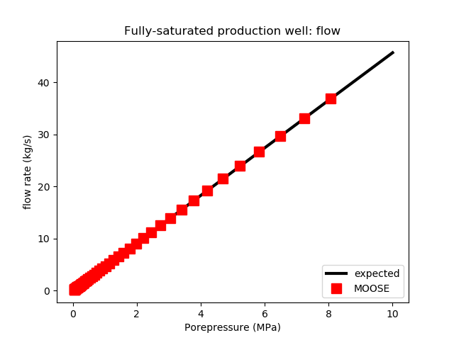
Figure 1: The flow to a production wellbore in MOOSE agrees with the expected result.
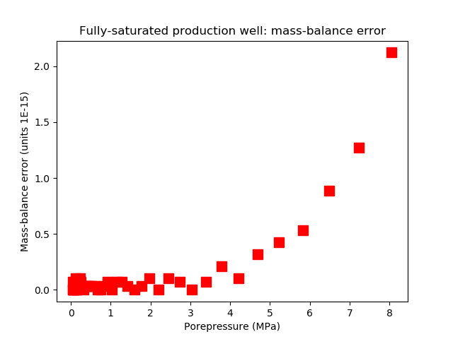
Figure 2: The mass-balance error is virtually zero.
An injection wellbore:
[DiracKernels<<<{"href": "../../syntax/DiracKernels/index.html"}>>>]
  [bh]
    type = PorousFlowPeacemanBorehole<<<{"description": "Approximates a borehole in the mesh using the Peaceman approach, ie using a number of point sinks with given radii whose positions are read from a file.  NOTE: if you are using PorousFlowPorosity that depends on volumetric strain, you should set strain_at_nearest_qp=true in your GlobalParams, to ensure the nodal Porosity Material uses the volumetric strain at the Dirac quadpoints, and can therefore be computed", "href": "../../source/dirackernels/PorousFlowPeacemanBorehole.html"}>>>
    variable<<<{"description": "The name of the variable that this residual object operates on"}>>> = pp
    SumQuantityUO<<<{"description": "User Object of type=PorousFlowSumQuantity in which to place the total outflow from the line sink for each time step."}>>> = borehole_total_outflow_mass
    point_file<<<{"description": "The file containing the coordinates of the points and their weightings that approximate the line sink.  The physical meaning of the weightings depend on the scenario, eg, they may be borehole radii.  Each line in the file must contain a space-separated weight and coordinate, viz r x y z.  For boreholes, the last point in the file is defined as the borehole bottom, where the borehole pressure is bottom_pressure.  If your file contains just one point, you must also specify the line_length and line_direction parameters.  Note that you will get segementation faults if your points do not lie within your mesh!"}>>> = bh03.bh
    function_of<<<{"description": "Modifying functions will be a function of either pressure and permeability (eg, for boreholes that pump fluids) or temperature and thermal conductivity (eg, for boreholes that pump pure heat with no fluid flow)"}>>> = pressure
    fluid_phase<<<{"description": "The fluid phase whose pressure (and potentially mobility, enthalpy, etc) controls the flux to the line sink.  For p_or_t=temperature, and without any use_*, this parameter is irrelevant"}>>> = 0
    bottom_p_or_t<<<{"description": "For function_of=pressure, this function is the pressure at the bottom of the borehole, otherwise it is the temperature at the bottom of the borehole."}>>> = 'insitu_pp'
    unit_weight<<<{"description": "(fluid_density*gravitational_acceleration) as a vector pointing downwards.  Note that the borehole pressure at a given z position is bottom_p_or_t + unit_weight*(q - q_bottom), where q=(x,y,z) and q_bottom=(x,y,z) of the bottom point of the borehole.  The analogous formula holds for function_of=temperature.  If you don't want bottomhole pressure (or temperature) to vary in the borehole just set unit_weight=0.  Typical value is = (0,0,-1E4), for water"}>>> = '0 0 0'
    use_mobility<<<{"description": "Multiply the flux by the fluid mobility"}>>> = true
    character<<<{"description": "If zero then borehole does nothing.  If positive the borehole acts as a sink (production well) for porepressure > borehole pressure, and does nothing otherwise.  If negative the borehole acts as a source (injection well) for porepressure < borehole pressure, and does nothing otherwise.  The flow rate to/from the borehole is multiplied by |character|, so usually character = +/- 1, but you can specify other quantities to provide an overall scaling to the flow if you like."}>>> = -1
  []
[]with a fully-saturated medium yields the correct result (Figure 3 and Figure 4):
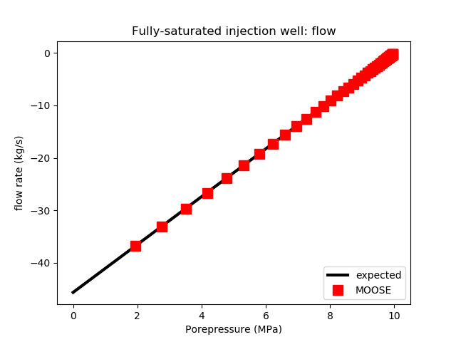
Figure 3: The flow from an injection wellbore in MOOSE agrees with the expected result.
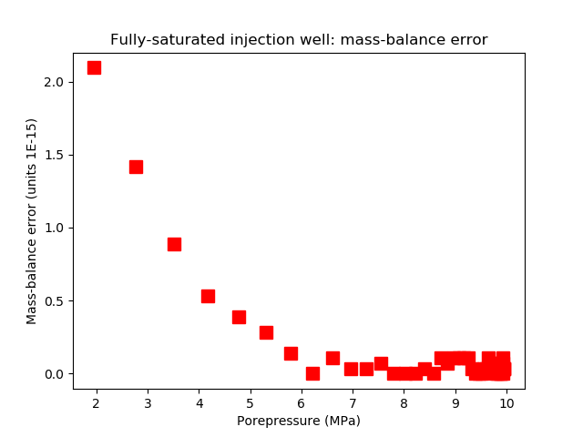
Figure 4: The mass-balance error is virtually zero.
A production wellbore with bottomhole porepressure MPa so it forces desaturation of an initially-saturated medium:
[DiracKernels<<<{"href": "../../syntax/DiracKernels/index.html"}>>>]
  [bh]
    type = PorousFlowPeacemanBorehole<<<{"description": "Approximates a borehole in the mesh using the Peaceman approach, ie using a number of point sinks with given radii whose positions are read from a file.  NOTE: if you are using PorousFlowPorosity that depends on volumetric strain, you should set strain_at_nearest_qp=true in your GlobalParams, to ensure the nodal Porosity Material uses the volumetric strain at the Dirac quadpoints, and can therefore be computed", "href": "../../source/dirackernels/PorousFlowPeacemanBorehole.html"}>>>
    variable<<<{"description": "The name of the variable that this residual object operates on"}>>> = pp
    SumQuantityUO<<<{"description": "User Object of type=PorousFlowSumQuantity in which to place the total outflow from the line sink for each time step."}>>> = borehole_total_outflow_mass
    point_file<<<{"description": "The file containing the coordinates of the points and their weightings that approximate the line sink.  The physical meaning of the weightings depend on the scenario, eg, they may be borehole radii.  Each line in the file must contain a space-separated weight and coordinate, viz r x y z.  For boreholes, the last point in the file is defined as the borehole bottom, where the borehole pressure is bottom_pressure.  If your file contains just one point, you must also specify the line_length and line_direction parameters.  Note that you will get segementation faults if your points do not lie within your mesh!"}>>> = bh02.bh
    fluid_phase<<<{"description": "The fluid phase whose pressure (and potentially mobility, enthalpy, etc) controls the flux to the line sink.  For p_or_t=temperature, and without any use_*, this parameter is irrelevant"}>>> = 0
    bottom_p_or_t<<<{"description": "For function_of=pressure, this function is the pressure at the bottom of the borehole, otherwise it is the temperature at the bottom of the borehole."}>>> = -1E6
    unit_weight<<<{"description": "(fluid_density*gravitational_acceleration) as a vector pointing downwards.  Note that the borehole pressure at a given z position is bottom_p_or_t + unit_weight*(q - q_bottom), where q=(x,y,z) and q_bottom=(x,y,z) of the bottom point of the borehole.  The analogous formula holds for function_of=temperature.  If you don't want bottomhole pressure (or temperature) to vary in the borehole just set unit_weight=0.  Typical value is = (0,0,-1E4), for water"}>>> = '0 0 0'
    use_mobility<<<{"description": "Multiply the flux by the fluid mobility"}>>> = true
    character<<<{"description": "If zero then borehole does nothing.  If positive the borehole acts as a sink (production well) for porepressure > borehole pressure, and does nothing otherwise.  If negative the borehole acts as a source (injection well) for porepressure < borehole pressure, and does nothing otherwise.  The flow rate to/from the borehole is multiplied by |character|, so usually character = +/- 1, but you can specify other quantities to provide an overall scaling to the flow if you like."}>>> = 1
  []
[]yields the correct result (Figure 5 and Figure 6):
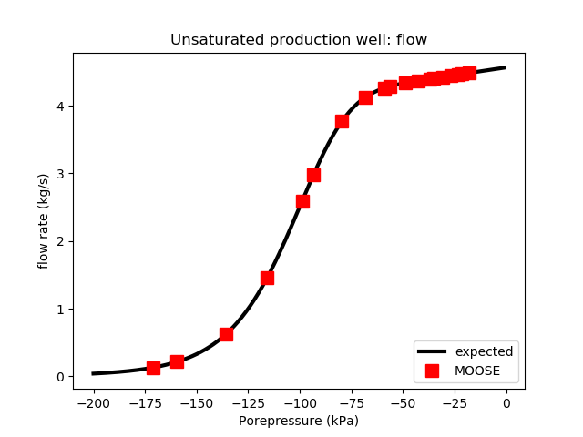
Figure 5: The flow to a production wellbore in MOOSE agrees with the expected result.
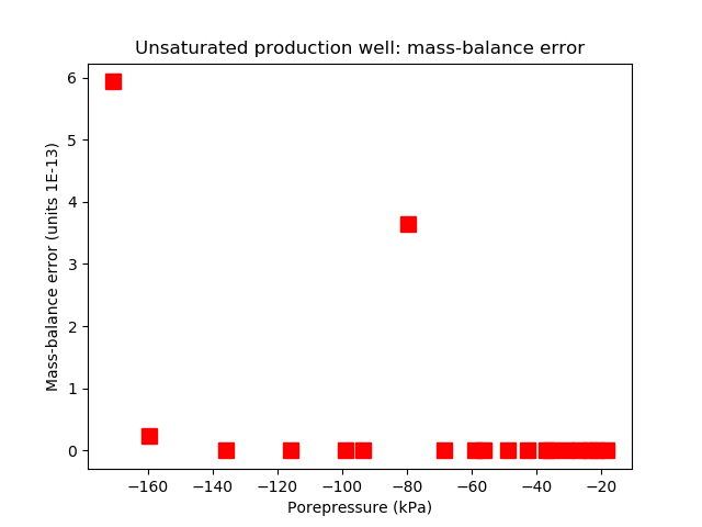
Figure 6: The mass-balance error is virtually zero.
An injection wellbore with so it is only active when the rock porepressure is negative:
[DiracKernels<<<{"href": "../../syntax/DiracKernels/index.html"}>>>]
  [bh]
    type = PorousFlowPeacemanBorehole<<<{"description": "Approximates a borehole in the mesh using the Peaceman approach, ie using a number of point sinks with given radii whose positions are read from a file.  NOTE: if you are using PorousFlowPorosity that depends on volumetric strain, you should set strain_at_nearest_qp=true in your GlobalParams, to ensure the nodal Porosity Material uses the volumetric strain at the Dirac quadpoints, and can therefore be computed", "href": "../../source/dirackernels/PorousFlowPeacemanBorehole.html"}>>>
    variable<<<{"description": "The name of the variable that this residual object operates on"}>>> = pp
    SumQuantityUO<<<{"description": "User Object of type=PorousFlowSumQuantity in which to place the total outflow from the line sink for each time step."}>>> = borehole_total_outflow_mass
    point_file<<<{"description": "The file containing the coordinates of the points and their weightings that approximate the line sink.  The physical meaning of the weightings depend on the scenario, eg, they may be borehole radii.  Each line in the file must contain a space-separated weight and coordinate, viz r x y z.  For boreholes, the last point in the file is defined as the borehole bottom, where the borehole pressure is bottom_pressure.  If your file contains just one point, you must also specify the line_length and line_direction parameters.  Note that you will get segementation faults if your points do not lie within your mesh!"}>>> = bh03.bh
    fluid_phase<<<{"description": "The fluid phase whose pressure (and potentially mobility, enthalpy, etc) controls the flux to the line sink.  For p_or_t=temperature, and without any use_*, this parameter is irrelevant"}>>> = 0
    bottom_p_or_t<<<{"description": "For function_of=pressure, this function is the pressure at the bottom of the borehole, otherwise it is the temperature at the bottom of the borehole."}>>> = 0
    unit_weight<<<{"description": "(fluid_density*gravitational_acceleration) as a vector pointing downwards.  Note that the borehole pressure at a given z position is bottom_p_or_t + unit_weight*(q - q_bottom), where q=(x,y,z) and q_bottom=(x,y,z) of the bottom point of the borehole.  The analogous formula holds for function_of=temperature.  If you don't want bottomhole pressure (or temperature) to vary in the borehole just set unit_weight=0.  Typical value is = (0,0,-1E4), for water"}>>> = '0 0 0'
    use_mobility<<<{"description": "Multiply the flux by the fluid mobility"}>>> = true
    character<<<{"description": "If zero then borehole does nothing.  If positive the borehole acts as a sink (production well) for porepressure > borehole pressure, and does nothing otherwise.  If negative the borehole acts as a source (injection well) for porepressure < borehole pressure, and does nothing otherwise.  The flow rate to/from the borehole is multiplied by |character|, so usually character = +/- 1, but you can specify other quantities to provide an overall scaling to the flow if you like."}>>> = -1
  []
[]yields the correct result for an initially unsaturated medium (Figure 7 and Figure 8):
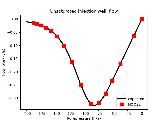
Figure 7: The flow from an injection wellbore in MOOSE agrees with the expected result.
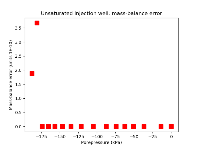
Figure 8: The mass-balance error is virtually zero.
Each of these record the total fluid flux (kg) injected by or produced by the borehole in a PorousFlowSumQuantity UserObject and outputs this result using a PorousFlowPlotQuantity Postprocessor:
  [borehole_total_outflow_mass]
    type = PorousFlowSumQuantity
[] [bh_report]
type = PorousFlowPlotQuantity
uo = borehole_total_outflow_mass
[]Reproducing the steady-state 2D analytical solution
The PorousFlow fluid equation (see governing equations) for a fully-saturated medium with and large constant bulk modulus becomes Darcy's equation where , with notation described in the nomenclature. In the isotropic case (where ), the steadystate equation is just Laplace's equation
Place a borehole of radius and infinite length oriented along the axis. Then the situation becomes 2D and can be solved in cylindrical coordinates, with and independent of . If the pressure at the borehole wall is , then the fluid density is . Assume that at the fluid pressure is held fixed at , or equivalently the density is held fixed at . Then the solution of Laplace's equation is well-known to be (5) This is the fundamental solution used by Peaceman and others to derive expressions for by comparing with numerical expressions resulting from Eq. (4).
Chen and Zhang Chen and Zhang (2009) have derived an expression for in the case where this borehole is placed at a node in a square mesh. This test compares the MOOSE steadystate solution with a single borehole with defined by Chen and Zhang's formula (specifically, the re_constant needs to be changed from its default value) is compared with Eq. (5) to illustrate that the MOOSE implementation of a borehole is correct.
The PorousFlowPeacemanBorehole is:
[DiracKernels<<<{"href": "../../syntax/DiracKernels/index.html"}>>>]
  [bh]
    type = PorousFlowPeacemanBorehole<<<{"description": "Approximates a borehole in the mesh using the Peaceman approach, ie using a number of point sinks with given radii whose positions are read from a file.  NOTE: if you are using PorousFlowPorosity that depends on volumetric strain, you should set strain_at_nearest_qp=true in your GlobalParams, to ensure the nodal Porosity Material uses the volumetric strain at the Dirac quadpoints, and can therefore be computed", "href": "../../source/dirackernels/PorousFlowPeacemanBorehole.html"}>>>
    variable<<<{"description": "The name of the variable that this residual object operates on"}>>> = pp
    SumQuantityUO<<<{"description": "User Object of type=PorousFlowSumQuantity in which to place the total outflow from the line sink for each time step."}>>> = borehole_total_outflow_mass
    point_file<<<{"description": "The file containing the coordinates of the points and their weightings that approximate the line sink.  The physical meaning of the weightings depend on the scenario, eg, they may be borehole radii.  Each line in the file must contain a space-separated weight and coordinate, viz r x y z.  For boreholes, the last point in the file is defined as the borehole bottom, where the borehole pressure is bottom_pressure.  If your file contains just one point, you must also specify the line_length and line_direction parameters.  Note that you will get segementation faults if your points do not lie within your mesh!"}>>> = bh07.bh
    fluid_phase<<<{"description": "The fluid phase whose pressure (and potentially mobility, enthalpy, etc) controls the flux to the line sink.  For p_or_t=temperature, and without any use_*, this parameter is irrelevant"}>>> = 0
    bottom_p_or_t<<<{"description": "For function_of=pressure, this function is the pressure at the bottom of the borehole, otherwise it is the temperature at the bottom of the borehole."}>>> = 0
    unit_weight<<<{"description": "(fluid_density*gravitational_acceleration) as a vector pointing downwards.  Note that the borehole pressure at a given z position is bottom_p_or_t + unit_weight*(q - q_bottom), where q=(x,y,z) and q_bottom=(x,y,z) of the bottom point of the borehole.  The analogous formula holds for function_of=temperature.  If you don't want bottomhole pressure (or temperature) to vary in the borehole just set unit_weight=0.  Typical value is = (0,0,-1E4), for water"}>>> = '0 0 0'
    use_mobility<<<{"description": "Multiply the flux by the fluid mobility"}>>> = true
    re_constant<<<{"description": "The dimensionless constant used in evaluating the borehole effective radius.  This depends on the meshing scheme.  Peacemann finite-difference calculations give 0.28, while for rectangular finite elements the result is closer to 0.1594.  (See  Eqn(4.13) of Z Chen, Y Zhang, Well flow models for various numerical methods, Int J Num Analysis and Modeling, 3 (2008) 375-388.)"}>>> = 0.1594 # use Chen and Zhang version
    character<<<{"description": "If zero then borehole does nothing.  If positive the borehole acts as a sink (production well) for porepressure > borehole pressure, and does nothing otherwise.  If negative the borehole acts as a source (injection well) for porepressure < borehole pressure, and does nothing otherwise.  The flow rate to/from the borehole is multiplied by |character|, so usually character = +/- 1, but you can specify other quantities to provide an overall scaling to the flow if you like."}>>> = 2 # double the strength because bh07.bh only fills half the mesh
  []
[]The mesh used is shown in Figure 9.
![The mesh used in the comparison with [eq:log_bh], with the green dot indicating the position of the borehole. The central elements are $10\times 10\,$m$^{2}$, and the outer boundary is at radius 300m.](../../media/porous_flow/bh07_mesh.png)
Figure 9: The mesh used in the comparison with Eq. (5), with the green dot indicating the position of the borehole. The central elements are m, and the outer boundary is at radius 300m.
Figure 10 show the comparison between the MOOSE result and Eq. (5). Most parameters in this study are identical to those given in the Table 1 with the following exceptions: the mesh is shown in Figure 9; the permeability is m; the borehole radius is 1 m; the borehole pressure is ; the outer radius is m; and the outer pressure is MPa.
![Comparison of the MOOSE results (dots) with the analytical solution [eq:log_bh] for the steadystate porepressure distribution surrounding single borehole.](../../media/porous_flow/bh07.png)
Figure 10: Comparison of the MOOSE results (dots) with the analytical solution Eq. (5) for the steadystate porepressure distribution surrounding single borehole.
Injecting and producing in thermo-hydro simulations
The PorousFlowPeacemanBorehole may be used to model injection and production in thermo-hydro simulations. Suppose that cool water is being injected into an initially hot reservoir via a vertical injection well, and that water is being removed from the system via a vertical production well. In this example we shall study an essentially 2D situation without gravity with parameters defined in Table 2
Table 2: Injection-production parameters
| Parameter | Value |
|---|---|
| Injection borehole radius | 0.2 m |
| Injection borehole vertical length | 10 m |
| Injection bottomhole pressure | 21 MPa |
| Injection temperature | 300 K |
| Production borehole radius | 0.25 m |
| Production borehole vertical length | 10 m |
| Production bottomhole pressure | 20 MPa |
| Injection-production well separation | 30 m |
| Reservoir initial porepressure | 20 MPa |
| Reservoir initial temperature | 400 K |
| Gravity | 0 |
| Unit fluid weight | 0 |
The fluid properties are defined as:
[FluidProperties<<<{"href": "../../syntax/FluidProperties/index.html"}>>>]
  [the_simple_fluid]
    type = SimpleFluidProperties<<<{"description": "Fluid properties for a simple fluid with a constant bulk density", "href": "../../source/fluidproperties/SimpleFluidProperties.html"}>>>
    thermal_expansion<<<{"description": "Constant coefficient of thermal expansion (1/K)"}>>> = 2E-4
    bulk_modulus<<<{"description": "Constant bulk modulus (Pa)"}>>> = 2E9
    viscosity<<<{"description": "Constant dynamic viscosity (Pa.s)"}>>> = 1E-3
    density0<<<{"description": "Density at zero pressure and zero temperature"}>>> = 1000
    cv<<<{"description": "Constant specific heat capacity at constant volume (J/kg/K)"}>>> = 4000.0
    cp<<<{"description": "Constant specific heat capacity at constant pressure (J/kg/K)"}>>> = 4000.0
  []
[]The fluid injection and production is implemented in a way that is now familiar:
  [fluid_injection]
    type = PorousFlowPeacemanBorehole
    variable = porepressure
    SumQuantityUO = injected_mass
    point_file = injection.bh
    function_of = pressure
    fluid_phase = 0
    bottom_p_or_t = 21E6
    unit_weight = '0 0 0'
    use_mobility = true
    character = -1
  []
  [fluid_production]
    type = PorousFlowPeacemanBorehole
    variable = porepressure
    SumQuantityUO = produced_mass
    point_file = production.bh
    function_of = pressure
    fluid_phase = 0
    bottom_p_or_t = 20E6
    unit_weight = '0 0 0'
    use_mobility = true
    character = 1
[]The injection temperature is set via:
[BCs<<<{"href": "../../syntax/BCs/index.html"}>>>]
  [injection_temperature]
    type = DirichletBC<<<{"description": "Imposes the essential boundary condition $u=g$, where $g$ is a constant, controllable value.", "href": "../../source/bcs/DirichletBC.html"}>>>
    variable<<<{"description": "The name of the variable that this residual object operates on"}>>> = temperature
    value<<<{"description": "Value of the BC"}>>> = 300
    boundary<<<{"description": "The list of boundary IDs from the mesh where this object applies"}>>> = central_nodes
  []
[]Alternatively, the heat energy of the injected fluid could be worked out and injected into the heat-conservation equation via a borehole.
The production of fluid means that heat energy must be removed at exactly the rate associated with the fluid-mass removal. This is implemented by using an identical PorousFlowPeacemanBorehole to the fluid production situation but associating it with the temperature variable and with use_enthalpy = true:
  [remove_heat_at_production_well]
    type = PorousFlowPeacemanBorehole
    variable = temperature
    SumQuantityUO = produced_heat
    point_file = production.bh
    function_of = pressure
    fluid_phase = 0
    bottom_p_or_t = 20E6
    unit_weight = '0 0 0'
    use_mobility = true
    use_enthalpy = true
    character = 1
Here the heat energy per timestep is saved into a PorousFlowSumQuantity UserObject which may be extracted using a PorousFlowPlotQuantity Postprocessor, which would be an important quantity in a geothermal application:
[Postprocessors<<<{"href": "../../syntax/Postprocessors/index.html"}>>>]
  [heat_joules_extracted_this_timestep]
    type = PorousFlowPlotQuantity<<<{"description": "Extracts the value from the PorousFlowSumQuantity UserObject", "href": "../../source/postprocessors/PorousFlowPlotQuantity.html"}>>>
    uo<<<{"description": "PorousFlowSumQuantity user object name that holds the required information"}>>> = produced_heat
  []
[]Scaling of the variables ensures good convergence:
[Variables<<<{"href": "../../syntax/Variables/index.html"}>>>]
  [porepressure]
    initial_condition<<<{"description": "Specifies a constant initial condition for this variable"}>>> = 20E6
  []
  [temperature]
    initial_condition<<<{"description": "Specifies a constant initial condition for this variable"}>>> = 400
    scaling<<<{"description": "Specifies a scaling factor to apply to this variable"}>>> = 1E-6 # fluid enthalpy is roughly 1E6
  []
[]Some results (run on a fine mesh) are shown in Figure 11 and Figure 12.
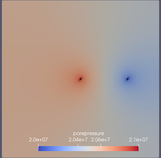
Figure 11: Porepressure after s of injection and production. The black spots indicate the wells.
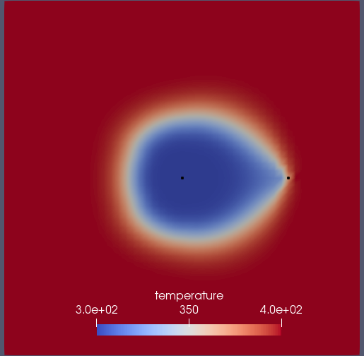
Figure 12: Temperature after s of injection and production. the black spots indicate the wells.
References
- Z. Chen and Y. Zhang.
Well flow models for various numerical methods.
International Journal of Numerical Analysis and Modelling, 6:375–388, 2009.[Export]
- D. W. Peaceman.
Interpretation of well-block pressures in numerical reservoir simulation with nonsquare grid blocks and anisotropic permeability.
SPE J., 23:531–543, 1983.[Export]