Boundary conditions
MOOSE's Dirichlet and Neumann boundary conditions enable simulation of simple scenarios. The Porous Flow module includes flexible boundary conditions that allow many different scenarios to be modelled. There are two classes of boundary conditions:
Those based on PorousFlowSink. These are typically used to add or remove fluid or heat-energy through the boundary. The basic sink adds/removes a fixed flux, but more elaborate sources/sinks add time-dependent fluxes, or fluxes dependent on fluid pressure or temperature, fluid mobility, enthalpy, etc. These boundary conditions may also be used to control porepressure, temperature, or mass fractions on the boundary by adding/removing fluid or heat through interaction with an external environment. It is often physically more correct and numerically advantageous to use these boundary conditions instead of DirichletBC.
Those based on PorousFlowOutflowBC, which is an "outflow" boundary condition that removes fluid components or heat energy as they flow to the boundary. This models a "free" boundary that is "invisible" to the simulation. Please see below for more description and warnings.
This page may be read in conjunction with the description of some of the tests of the PorousFlow sinks.
Class 1: Basic sink formulation
The basic sink is where is a MOOSE Function of time and position on the boundary.
If then the boundary condition will act as a sink, while if the boundary condition acts as a source. If applied to a fluid-component equation, the function has units kg.m.s. If applied to the heat equation, the function has units J.m.s. The units of are potentially modified if the extra building blocks enumerated below are used (but the units of the final result, , will always be kg.m.s or J.m.s).
If the fluid flow through the boundary is required, use the save_in command which will save the sink strength to an AuxVariable. This AuxVariable will be the flux (kg.s or J.s) from each node on the boundary, which is the product of and the area attributed to that node. If the total flux (kg.s or J.s) through the boundary is required, integrate the AuxVariable over the boundary using a NodalSum Postprocessor.
This basic sink boundary condition is implemented in PorousFlowSink.
Class 1: More elaborate options
The basic sink may be multiplied by a MOOSE Function of the pressure of a fluid phase or the temperature: (1) Here the units of are kg.m.s (for fluids) or J.m.s (for heat). and are reference values, that may be AuxVariables to allow spatial and temporal variance. Some commonly use forms have been hard-coded into the Porous Flow module for ease of use in simulations:
A piecewise linear function (for simulating fluid or heat exchange with an external environment via a conductivity term, for instance), implemented in
PorousFlowPiecewiseLinearSinkA half-gaussian (for simulating evapotranspiration, for instance), implemented in
PorousFlowHalfGaussianSinkA half-cubic (for simulating evapotranspiration, for example), implemented in
PorousFlowHalfCubicSink
In addition, the sink may be multiplied by any or all of the following quantities
Fluid relative permeability
Fluid mobility (, where is the normal vector to the boundary)
Fluid mass fraction
Fluid internal energy
Thermal conductivity
Class 1: Fixing fluid porepressures using the PorousFlowSink
Frequently in PorousFlow simulations fixing fluid porepressures using Dirichlet conditions is inappropriate.
Physically a Dirichlet condition corresponds to an environment outside a model providing a limitless source (or sink) of fluid and that does not happen in reality.
The Variables used may not be porepressure, so a straightforward translation to "fixing porepressure" is not easy.
The Dirichlet condition can lead to extremely poor convergence as it forces areas near the boundary close to unphysical or unlikely regions in parameter space.
Physical Intuition Behind PorousFlowSink
It is advantageous to think of what the boundary condition is physically trying to represent before using Dirichlet conditions, and often a PorousFlowSink is more appropriate to use. For instance, at the top of a groundwater-gas model, gas can freely enter the model from the atmosphere, and escape the model to the atmosphere, which may be modelled using a PorousFlowSink. Water can exit the model if the water porepressure increases above atmospheric pressure, but the recharge if porepressure is lowered may be zero. Again this may be modelled using a PorousFlowSink.
When fixing porepressures (or temperatures) using a PorousFlowSink, what should the "conductance" be? Consider an imaginary environment that sits at distance from the model. The imaginary environment provides a limitless source or sink of fluid, but that fluid must travel through the distance between the model and the imaginary environment. The flux of fluid from the model to this environment is (approximately) (2) A similar equation holds for temperature (but in PorousFlow simulations the heat is sometimes supplied by the fluid, in which case the appropriate equation to use for the heat may be the above equation multiplied by the enthalpy). Here is the permeability of the region between the model and the imaginary environment (which can also be thought of as the permeability of the adjacent element), is the relative permeability in this region, and are the fluid density and viscosity. The environment porepressure is and the boundary porepressure is .
If this effectively fixes the porepressure to , since the flux is very large otherwise (physically: fluid is rapidly removed or added to the system by the environment to ensure ). If the boundary flux is almost zero and does nothing.
Numerical Implementation
The PorousFlowSink is implemented in a fairly general way that allows for flexibility in setting combinations of pressure and temperature boundary conditions. Due to its implementation, it is difficult to draw a perfect analogy to the physical flux. Nevertheless, Eq. (2) may be implemented in a number of ways, and one of the most common involves a PorousFlowPiecewiseLinearSink that follows the format of Eq. (1) using and as a piecewise linear function between ordered pairs of pt_vals (on the x-axis) and multiplier (on the y-axis). An example of the function is shown in the figure below. It accepts as an input and returns a value that ends up multiplying to give a flux (as in Eq. (1)). can be thought of as the conductance and is specified with flux_function = C. Its numerical value is discussed below. can be specified using an AuxVariable or set to a constant value using PT_shift = Pe.
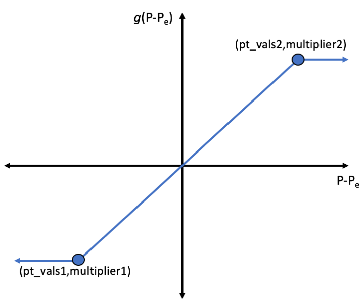
Figure 1: Depiction of for PorousFlowPiecewiseLinearSink. The function accepts as an input (i.e. the difference between a specified environment pressure and the pressure on the boundary element) and returns a value that multiplies to give the flux out of the domain.
To set a Dirichlet boundary condition , either or the slope of should be very large. It is usually convenient to make the slope of equal to 1 by setting pt_vals = '-1E9 1E9' and multipliers = '-1E9 1E9', and then can be selected appropriately. The range for pt_vals should be sufficiently large that the simulation always occupies the region between the values specified (-1E9 1E9 is a typical choice because porepressures encountered in many simulations are ). This ensures good convergence, and if in doubt set the pt_vals at a higher value than you expect. If falls outside of the range defined in pt_vals, then the slope of . This can be useful to set a boundary condition that will only allow for outflow (e.g. by using pt_vals = '0 1E9', multipliers = '0 1E9').`
The numerical value of the conductance, , is , must be set at an appropriate value for the model. Alternately, a PorousFlowPiecewiseLinearSink may be constructed with the same pt_vals, multipliers and PT_shift, but with use_mobility = true and use_relperm =
true, and then . This has three advantages: (1) the MOOSE input file is simpler; (2) MOOSE automatically chooses the correct mobility and relative permeability to use; (3) these parameters are appropriate to the model so it reduces the potential for difficult numerical situations occurring.
Also note, if is too large, the boundary residual will be much larger than residuals within the domain. This results in poor convergence.
So what value should be assigned to ? In the example below, , kg/m, m, , and Pa-s. Therefore m. This value of is small enough to ensure that the Dirichlet boundary condition is satisfied. If is increased to , m, and the simulation has difficulty converging. If , m, and the boundary acts like a source of fluid from a distant reservoir (i.e. it no longer acts like a Dirichlet boundary condition). The value of is simply if use_mobility = true and use_relperm = true.
[BCs<<<{"href": "../../syntax/BCs/index.html"}>>>]
  [in_left]
    type = PorousFlowPiecewiseLinearSink<<<{"description": "Applies a flux sink to a boundary. The base flux defined by PorousFlowSink is multiplied by a piecewise linear function.", "href": "../../source/bcs/PorousFlowPiecewiseLinearSink.html"}>>>
    variable<<<{"description": "The name of the variable that this residual object operates on"}>>> = porepressure
    boundary<<<{"description": "The list of boundary IDs from the mesh where this object applies"}>>> = 'left'
    pt_vals<<<{"description": "Tuple of pressure values (for the fluid_phase specified).  Must be monotonically increasing.  For heat fluxes that don't involve fluids, these are temperature values"}>>> = '-1e9 1e9' # x coordinates defining g
    multipliers<<<{"description": "Tuple of multiplying values.  The flux values are multiplied by these."}>>> = '-1e9 1e9' # y coordinates defining g
    PT_shift<<<{"description": "Whenever the sink is an explicit function of porepressure (such as a PiecewiseLinear function) the argument of the function is set to P - PT_shift instead of simply P.  Similarly for temperature.  PT_shift does not enter into any use_* calculations."}>>> = 2.E6   # BC pressure
    flux_function<<<{"description": "The flux.  The flux is OUT of the medium: hence positive values of this function means this BC will act as a SINK, while negative values indicate this flux will be a SOURCE.  The functional form is useful for spatially or temporally varying sinks.  Without any use_*, this function is measured in kg.m^-2.s^-1 (or J.m^-2.s^-1 for the case with only heat and no fluids)"}>>> = 1E-5 # Variable C
    fluid_phase<<<{"description": "If supplied, then this BC will potentially be a function of fluid pressure, and you can use mass_fraction_component, use_mobility, use_relperm, use_enthalpy and use_energy.  If not supplied, then this BC can only be a function of temperature"}>>> = 0
    save_in<<<{"description": "The name of auxiliary variables to save this BC's residual contributions to.  Everything about that variable must match everything about this variable (the type, what blocks it's on, etc.)"}>>> = fluxes_out
  []
  [out_right]
    type = PorousFlowPiecewiseLinearSink<<<{"description": "Applies a flux sink to a boundary. The base flux defined by PorousFlowSink is multiplied by a piecewise linear function.", "href": "../../source/bcs/PorousFlowPiecewiseLinearSink.html"}>>>
    variable<<<{"description": "The name of the variable that this residual object operates on"}>>> = porepressure
    boundary<<<{"description": "The list of boundary IDs from the mesh where this object applies"}>>> = 'right'
    pt_vals<<<{"description": "Tuple of pressure values (for the fluid_phase specified).  Must be monotonically increasing.  For heat fluxes that don't involve fluids, these are temperature values"}>>> = '-1e9 1e9' # x coordinates defining g
    multipliers<<<{"description": "Tuple of multiplying values.  The flux values are multiplied by these."}>>> = '-1e9 1e9' # y coordinates defining g
    PT_shift<<<{"description": "Whenever the sink is an explicit function of porepressure (such as a PiecewiseLinear function) the argument of the function is set to P - PT_shift instead of simply P.  Similarly for temperature.  PT_shift does not enter into any use_* calculations."}>>> = 1.E6   # BC pressure
    flux_function<<<{"description": "The flux.  The flux is OUT of the medium: hence positive values of this function means this BC will act as a SINK, while negative values indicate this flux will be a SOURCE.  The functional form is useful for spatially or temporally varying sinks.  Without any use_*, this function is measured in kg.m^-2.s^-1 (or J.m^-2.s^-1 for the case with only heat and no fluids)"}>>> = 1E-6 # Variable C
    fluid_phase<<<{"description": "If supplied, then this BC will potentially be a function of fluid pressure, and you can use mass_fraction_component, use_mobility, use_relperm, use_enthalpy and use_energy.  If not supplied, then this BC can only be a function of temperature"}>>> = 0
    save_in<<<{"description": "The name of auxiliary variables to save this BC's residual contributions to.  Everything about that variable must match everything about this variable (the type, what blocks it's on, etc.)"}>>> = fluxes_in
  []
[]Class 1: Injection of fluid at a fixed temperature
A boundary condition corresponding to injection of fluid at a fixed temperature could involve: (1) using a Dirichlet condition for temperature; (2) using without any multiplicative factors. More complicated examples with heat and fluid injection and production are detailed in the test suite documentation.
Class 1: Fluids that both enter and exit the boundary
Commonly, if fluid or heat is exiting the porous material, multiplication by relative permeability, mobility, mass fraction, enthalpy or thermal conductivity is necessary, while if fluid or heat is entering the porous material this multiplication is not necessary. Two sinks can be constructed in a MOOSE input file: one involving production which is only active for using a Piecewise-linear sink (here is the environmental pressure); and one involving injection, which is only active for using a piecewise-linear sink multiplied by the appropriate factors.
Class 1: A 2-phase example
To illustrate that the "sink" part of the PorousFlowSink boundary condition works as planned, consider 2-phase flow along a line. (A similar problem using the PorousFlowOutflowBCs is described below.) The simulation is initially saturated with water, and CO is injected at the left-side. The CO front moves towards the right, but what boundary conditions should be placed on the right so that they don't interfere with the flow?
The answer is that two PorousFlowPiecewiseLinearSink are needed. One pulls out water and the other pulls out CO. They extract the fluids in proportion to their mass fractions, mobilities and relative permeabilities, in the way described above. Let us explore the input file a little.
In this example there are two fluid components:
fluid component 0 is water
fluid component 1 is CO
and two phases:
phase 0 is liquid
phase 1 is gas
The water component only exists in the liquid phase and the CO component only exists in the gaseous phase (the fluids are immiscible). The Variables are the water and gas porepressures:
[Variables<<<{"href": "../../syntax/Variables/index.html"}>>>]
  [pwater]
    initial_condition<<<{"description": "Specifies a constant initial condition for this variable"}>>> = 20E6
  []
  [pgas]
    initial_condition<<<{"description": "Specifies a constant initial condition for this variable"}>>> = 20.1E6
  []
[]The pwater Variable is associated with the water component, while the pgas Variable is associated with the CO component:
[Kernels<<<{"href": "../../syntax/Kernels/index.html"}>>>]
  [mass0]
    type = PorousFlowMassTimeDerivative<<<{"description": "Derivative of fluid-component mass with respect to time.  Mass lumping to the nodes is used.", "href": "../../source/kernels/PorousFlowMassTimeDerivative.html"}>>>
    fluid_component<<<{"description": "The index corresponding to the component for this kernel"}>>> = 0
    variable<<<{"description": "The name of the variable that this residual object operates on"}>>> = pwater
  []
  [flux0]
    type = PorousFlowAdvectiveFlux<<<{"description": "Fully-upwinded advective flux of the component given by fluid_component", "href": "../../source/kernels/PorousFlowAdvectiveFlux.html"}>>>
    fluid_component<<<{"description": "The index corresponding to the fluid component for this kernel"}>>> = 0
    variable<<<{"description": "The name of the variable that this residual object operates on"}>>> = pwater
  []
  [mass1]
    type = PorousFlowMassTimeDerivative<<<{"description": "Derivative of fluid-component mass with respect to time.  Mass lumping to the nodes is used.", "href": "../../source/kernels/PorousFlowMassTimeDerivative.html"}>>>
    fluid_component<<<{"description": "The index corresponding to the component for this kernel"}>>> = 1
    variable<<<{"description": "The name of the variable that this residual object operates on"}>>> = pgas
  []
  [flux1]
    type = PorousFlowAdvectiveFlux<<<{"description": "Fully-upwinded advective flux of the component given by fluid_component", "href": "../../source/kernels/PorousFlowAdvectiveFlux.html"}>>>
    fluid_component<<<{"description": "The index corresponding to the fluid component for this kernel"}>>> = 1
    variable<<<{"description": "The name of the variable that this residual object operates on"}>>> = pgas
  []
[]A van Genuchten capillary pressure is used
  [pc]
    type = PorousFlowCapillaryPressureVG
    alpha = 1E-6
    m = 0.6
The remainder of the input file is pretty standard, save for the important BCs block:
[BCs<<<{"href": "../../syntax/BCs/index.html"}>>>]
  [co2_injection]
    type = PorousFlowSink<<<{"description": "Applies a flux sink to a boundary.", "href": "../../source/bcs/PorousFlowSink.html"}>>>
    boundary<<<{"description": "The list of boundary IDs from the mesh where this object applies"}>>> = left
    variable<<<{"description": "The name of the variable that this residual object operates on"}>>> = pgas # pgas is associated with the CO2 mass balance (fluid_component = 1 in its Kernels)
    flux_function<<<{"description": "The flux.  The flux is OUT of the medium: hence positive values of this function means this BC will act as a SINK, while negative values indicate this flux will be a SOURCE.  The functional form is useful for spatially or temporally varying sinks.  Without any use_*, this function is measured in kg.m^-2.s^-1 (or J.m^-2.s^-1 for the case with only heat and no fluids)"}>>> = -1E-2 # negative means a source, rather than a sink
  []

  [right_water]
    type = PorousFlowPiecewiseLinearSink<<<{"description": "Applies a flux sink to a boundary. The base flux defined by PorousFlowSink is multiplied by a piecewise linear function.", "href": "../../source/bcs/PorousFlowPiecewiseLinearSink.html"}>>>
    boundary<<<{"description": "The list of boundary IDs from the mesh where this object applies"}>>> = right

    # a sink of water, since the Kernels given to pwater are for fluid_component = 0 (the water)
    variable<<<{"description": "The name of the variable that this residual object operates on"}>>> = pwater

    # this Sink is a function of liquid porepressure
    # Also, all the mass_fraction, mobility and relperm are referenced to the liquid phase now
    fluid_phase<<<{"description": "If supplied, then this BC will potentially be a function of fluid pressure, and you can use mass_fraction_component, use_mobility, use_relperm, use_enthalpy and use_energy.  If not supplied, then this BC can only be a function of temperature"}>>> = 0

    # Sink strength = (Pwater - 20E6)
    pt_vals<<<{"description": "Tuple of pressure values (for the fluid_phase specified).  Must be monotonically increasing.  For heat fluxes that don't involve fluids, these are temperature values"}>>> = '0 1E9'
    multipliers<<<{"description": "Tuple of multiplying values.  The flux values are multiplied by these."}>>> = '0 1E9'
    PT_shift<<<{"description": "Whenever the sink is an explicit function of porepressure (such as a PiecewiseLinear function) the argument of the function is set to P - PT_shift instead of simply P.  Similarly for temperature.  PT_shift does not enter into any use_* calculations."}>>> = 20E6

    # multiply Sink strength computed above by mass fraction of water at the boundary
    mass_fraction_component<<<{"description": "The index corresponding to a fluid component.  If supplied, the flux will be multiplied by the nodal mass fraction for the component"}>>> = 0

    # also multiply Sink strength by mobility of the liquid
    use_mobility<<<{"description": "If true, then fluxes are multiplied by (density*permeability_nn/viscosity), where the '_nn' indicates the component normal to the boundary.  In this case bare_flux is measured in Pa.m^-1.  This can be used in conjunction with other use_*"}>>> = true

    # also multiply Sink strength by the relperm of the liquid
    use_relperm<<<{"description": "If true, then fluxes are multiplied by relative permeability.  This can be used in conjunction with other use_*"}>>> = true

    # also multiplly Sink strength by 1/L, where L is the distance to the fixed-porepressure external environment
    flux_function<<<{"description": "The flux.  The flux is OUT of the medium: hence positive values of this function means this BC will act as a SINK, while negative values indicate this flux will be a SOURCE.  The functional form is useful for spatially or temporally varying sinks.  Without any use_*, this function is measured in kg.m^-2.s^-1 (or J.m^-2.s^-1 for the case with only heat and no fluids)"}>>> = 10 # 1/L
  []

  [right_co2]
    type = PorousFlowPiecewiseLinearSink<<<{"description": "Applies a flux sink to a boundary. The base flux defined by PorousFlowSink is multiplied by a piecewise linear function.", "href": "../../source/bcs/PorousFlowPiecewiseLinearSink.html"}>>>
    boundary<<<{"description": "The list of boundary IDs from the mesh where this object applies"}>>> = right
    variable<<<{"description": "The name of the variable that this residual object operates on"}>>> = pgas
    fluid_phase<<<{"description": "If supplied, then this BC will potentially be a function of fluid pressure, and you can use mass_fraction_component, use_mobility, use_relperm, use_enthalpy and use_energy.  If not supplied, then this BC can only be a function of temperature"}>>> = 1
    pt_vals<<<{"description": "Tuple of pressure values (for the fluid_phase specified).  Must be monotonically increasing.  For heat fluxes that don't involve fluids, these are temperature values"}>>> = '0 1E9'
    multipliers<<<{"description": "Tuple of multiplying values.  The flux values are multiplied by these."}>>> = '0 1E9'
    PT_shift<<<{"description": "Whenever the sink is an explicit function of porepressure (such as a PiecewiseLinear function) the argument of the function is set to P - PT_shift instead of simply P.  Similarly for temperature.  PT_shift does not enter into any use_* calculations."}>>> = 20.1E6
    mass_fraction_component<<<{"description": "The index corresponding to a fluid component.  If supplied, the flux will be multiplied by the nodal mass fraction for the component"}>>> = 1
    use_mobility<<<{"description": "If true, then fluxes are multiplied by (density*permeability_nn/viscosity), where the '_nn' indicates the component normal to the boundary.  In this case bare_flux is measured in Pa.m^-1.  This can be used in conjunction with other use_*"}>>> = true
    use_relperm<<<{"description": "If true, then fluxes are multiplied by relative permeability.  This can be used in conjunction with other use_*"}>>> = true
    flux_function<<<{"description": "The flux.  The flux is OUT of the medium: hence positive values of this function means this BC will act as a SINK, while negative values indicate this flux will be a SOURCE.  The functional form is useful for spatially or temporally varying sinks.  Without any use_*, this function is measured in kg.m^-2.s^-1 (or J.m^-2.s^-1 for the case with only heat and no fluids)"}>>> = 10 # 1/L
  []
[]Below are shown some outputs. Evidently the boundary condition satisfies the requirements.
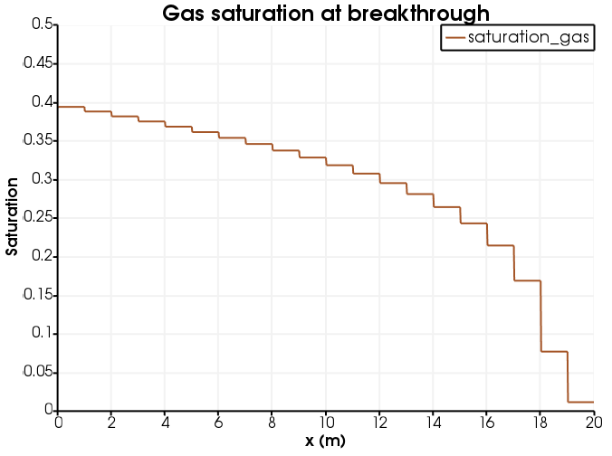
Figure 2: Gas saturation at breakthrough (the jaggedness of the line is because gas saturation is an elemental variable).
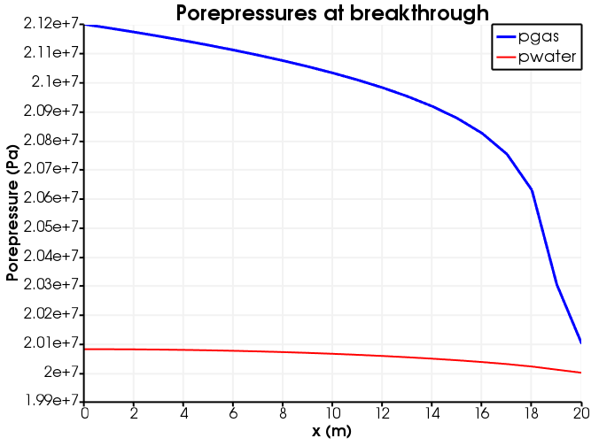
Figure 3: Porepressures at breakthrough.
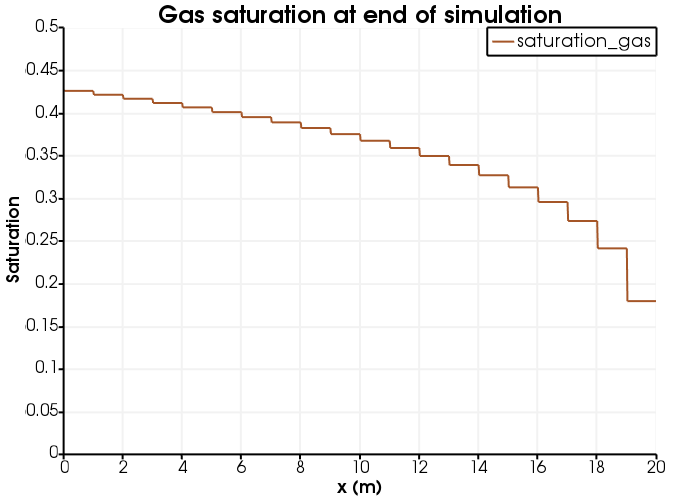
Figure 4: Gas saturation at the end of simulation.
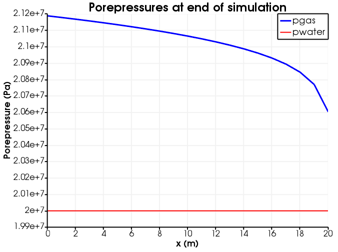
Figure 5: Porepressures at the end of simulation.
Figure 6: Evolution of gas saturation (the jaggedness of the line is because gas saturation is an elemental variable).
Class 2: Boundary terms for advection-diffusion equations
The theoretical background concerning boundary fluxes is developed in this section. The initial part of the presentation is general and not specific to Porous Flow. The variable may represent temperature, fluid mass, mass-density of a species, number-density of a species, etc. The flux quantified below has units depending on the physical meaning of : if is temperature then the flux has units J.s; if is fluid mass then the flux has units kg.s, etc. For sake or argument, is referred to as "fluid" in the discussion below.
The advection equation
The advection equation for is The velocity field advects , meaning that follows the streamlines of . The weak form of this equation reads (3) In a MOOSE input file, the second term is typically represented by a ConservativeAdvection Kernel, while the final term is the flux out through the surface and can be represented by an Outflow or Inflow BC.
The flux out through an area is Here is the outward normal to . If is an arbitrary internal area, this equation is always correct, but if is on the boundary of the simulation, the flux out is dictated by the boundary condition used.
There are various common boundary conditions. For the sake of the arguments below, imagine being an outside boundary of the MOOSE numerical model.
If then fluid is moving from the numerical model through the boundary towards the outside of the model. If no BC is used then there is no term in the system of equations that is removing fluid from the boundary. That is, no fluid is allowed out of the model through , and fluid builds up at the boundary. (Even though , does not have to be zero on the boundary.)
If then fluid is moving from the numerical model through the boundary towards the outside of the model. An
OutflowBC is exactly the final term in Eq. (3). This removes fluid through at exactly the rate specified by the advection equation, so this is a "free" boundary that is "invisible" to the simulation.If then fluid is moving from outside the model through the boundary and into the model. However, if no BC is used then no fluid enters the domain through (and will reduce).
If then fluid is moving from outside the model through the boundary and into the model. An
InflowBC, which is exactly the last term in Eq. (3) with fixed, may be used to specify an injection rate through this boundary ( has units kg.s.m).
The diffusion equation
The diffusion equation for (representing temperature, fluid mass, mass-density of a species, etc) is with weak form (4) The second is typically represented in MOOSE using the Diffusion Kernel, while the last term is the DiffusionFluxBC BC (assuming ). This last term is the flux out (kg.s, or J.s, or whatever are appropriate units associated with ) through an area .
The flux out through an arbitrary area is Here is the outward normal to . If is an arbitrary internal area, this equation is always correct, but if is on the boundary of the simulation, the flux out is dictated by the boundary condition used.
Inclusion of a BC for in a MOOSE input file will specify something about the flux from the boundary. Some examples are:
A
NeumannBCsimply adds a constant value (kg.s.m) to the Residual and integrates it over the boundary. Adding this constant value corresponds to adding a constant flux of fluid and MOOSE will find the solution that has . The value is the flux into the domain (negative of the out-going flux mentioned above).Using no BC at all on means that there is no boundary term in Eq. (4) so no fluid gets removed from this boundary: it is impermeable. MOOSE will find the solution that has .
Using a
DirichletBCfixes on the boundary. The physical interpretation is that an external source or sink is providing or removing fluid at the correct rate so that remains fixed.Using a
DiffusionFluxBCwill remove fluid at exactly the rate specified by the diffusion equation (assuming : otherwise an extension to the DiffusionFluxBC class needs to be encoded into MOOSE). This boundary condition is a "free" boundary that is "invisible" to the simulation.
The advection-diffusion equation
The advection-diffusion equation for (representing temperature, fluid mass, mass-density of a species, etc) is just a combination of the above: with weak form (5)
The flux out (kg.s, or J.s, or whatever are appropriate units associated with ) through an area is Here is the outward normal to .
Inclusion of a BC for in a MOOSE input file will specify something about the flux from the boundary. Some examples are.
Using no BCs means the final term Eq. (5) is missing from the system of equations that MOOSE solves. This means that no fluid is entering or exiting the domain from this boundary: the boundary is "impermeable". The fluid will "pile up" at the boundary, if is such that it is attempting to "blow" fluid out of the boundary (). Conversely, the fluid will deplete at the boundary, if is attempting to "blow" fluid from the boundary into the model domain ().
A
NeumannBCadds a constant value (kg.s.m) to the Residual and integrates it over the boundary. Adding this constant value corresponds to adding a constant flux of fluid and MOOSE will find the solution that has . The value of is the flux into the domain (negative of the out-going flux mentioned above).Using an
OutflowBCtogether with aDiffusionFluxBCremoves fluid through at exactly the rate specified by the advection-diffusion equation, so this is a "free" boundary that is "invisible" to the simulation.
The PorousFlow mass flux
The governing equation for mass conservation of fluid species is The standard PorousFlow nomenclature as been used here. The weak form is (6) The flux of species out through an arbitrary area is This has SI units kg.s.
Inclusion of a BC for porepressure or mass fraction in a MOOSE input file will specify something about the flux from the boundary.
Using no BCs means the final term Eq. (6) is missing from the system of equations that MOOSE solves, in other words, it is zero. Hence, no fluid is entering or exiting the domain from this boundary: the boundary is "impermeable", and MOOSE will find the solution .
A
NeumannBCadds a constant value, , (kg.s.m) to the Residual and integrates it over the boundary. Adding this constant value corresponds to adding a constant flux of fluid species, and MOOSE will find the solution that has . The value of is the flux into the domain (negative of the out-going flux mentioned above).Any of the PorousFlowSink variants mentioned above act in the same way as the NeumannBC by adding a value to the Residual and integrating it over the boundary, thereby allowing flux through the boundary to be specified. However, the PorousFlowSink variants are much more flexible than any of the NeumannBC variants that are coded into the MOOSE framework, so should be preferred in PorousFlow simulations.
Fixing the porepressure or mass fraction with a DirichletBC is also possible. This corresponds to adding/removing fluid species to keep the porepressure or mass fraction fixed, which can lead to severe numerical problems (for instance, trying to remove a fluid species that has zero mass fraction) so DirichletBC should be used with caution in PorousFlow simulations. Instead, one of the PorousFlowSink variants should usually be used, as described in detail above.
Using a PorousFlowOutflowBC removes fluid species through at exactly the rate specified by the Darcy equation Eq. (6), so this is a "free" boundary that is "invisible" to the simulation. More details are given below.
The PorousFlow heat flux
The governing equation for heat-energy conservation is The standard PorousFlow nomenclature as been used here. The weak form is (7) The flux of heat energy out through an arbitrary area is This has SI units J.s. Analogous remarks to the mass-flow case can be made concerning possible different types of BC.
Class 2: The PorousFlowOutflowBC
The PorousFlowOutflowBC adds the following term to the residual Various forms of may be chosen, as discussed in the PorousFlowOutflowBC documentation, so that this BC removes fluid species or heat energy through at exactly the rate specified by the Darcy equation Eq. (6) or the heat equation Eq. (7). Therefore, this BC can be used to represent a "free" boundary through which fluid or heat can freely flow: the boundary is "invisible" to the simulation.
Ensure your normal vector points out of the model, otherwise your fluxes will have the wrong sign.
PorousFlowOutflowBC does not model the interface of the model with "empty space". Imagine a model of a porous-media pipe containing water. PorousFlowOutflowBC does not model the situation where the pipe has an end through which the water flows into empty space. Instead, PorousFlowOutflowBC allows only part of the pipe to be modelled: when water exits the model it continues freely into the unmodelled section of the pipe. In this sense, the model's boundary is "invisible" to the simulation. This has a further consequence: if there is a sink in the modelled section, PorousFlowOutflowBC will allow water to flow from the unmodelled section into the modelled section.
The rate of outflow is limited by the permeability, the viscosity of the fluid, etc, in exactly the same way that the Darcy velocity is limited by these quantities. This means, for instance, if you inject a lot of fluid or heat into the model, it will take the PorousFlowOutflowBC some time to "suck" it all out.
Example: a 2-phase model
This example is similar to the 2-phase model employing a set of PorousFlowPiecewiseLinearSinks described above. Consider 2-phase flow along a line. This time, both water and CO are injected from the left boundary, while the right boundary has two PorousFlowOutflowBCs.
In this example there are two fluid components:
fluid component 0 is water
fluid component 1 is CO
and two phases:
phase 0 is liquid
phase 1 is gas
The water component only exists in the liquid phase and the CO component only exists in the gaseous phase (the fluids are immiscible). The Variables are the water and gas porepressures:
[Variables<<<{"href": "../../syntax/Variables/index.html"}>>>]
  [pwater]
    initial_condition<<<{"description": "Specifies a constant initial condition for this variable"}>>> = 20E6
  []
  [pgas]
    initial_condition<<<{"description": "Specifies a constant initial condition for this variable"}>>> = 21E6
  []
[]The pwater Variable is associated with the water component, while the pgas Variable is associated with the CO component:
[Kernels<<<{"href": "../../syntax/Kernels/index.html"}>>>]
  [mass0]
    type = PorousFlowMassTimeDerivative<<<{"description": "Derivative of fluid-component mass with respect to time.  Mass lumping to the nodes is used.", "href": "../../source/kernels/PorousFlowMassTimeDerivative.html"}>>>
    fluid_component<<<{"description": "The index corresponding to the component for this kernel"}>>> = 0
    variable<<<{"description": "The name of the variable that this residual object operates on"}>>> = pwater
  []
  [flux0]
    type = PorousFlowAdvectiveFlux<<<{"description": "Fully-upwinded advective flux of the component given by fluid_component", "href": "../../source/kernels/PorousFlowAdvectiveFlux.html"}>>>
    fluid_component<<<{"description": "The index corresponding to the fluid component for this kernel"}>>> = 0
    variable<<<{"description": "The name of the variable that this residual object operates on"}>>> = pwater
  []
  [mass1]
    type = PorousFlowMassTimeDerivative<<<{"description": "Derivative of fluid-component mass with respect to time.  Mass lumping to the nodes is used.", "href": "../../source/kernels/PorousFlowMassTimeDerivative.html"}>>>
    fluid_component<<<{"description": "The index corresponding to the component for this kernel"}>>> = 1
    variable<<<{"description": "The name of the variable that this residual object operates on"}>>> = pgas
  []
  [flux1]
    type = PorousFlowAdvectiveFlux<<<{"description": "Fully-upwinded advective flux of the component given by fluid_component", "href": "../../source/kernels/PorousFlowAdvectiveFlux.html"}>>>
    fluid_component<<<{"description": "The index corresponding to the fluid component for this kernel"}>>> = 1
    variable<<<{"description": "The name of the variable that this residual object operates on"}>>> = pgas
  []
[]The remainder of the input file is pretty standard, save for the important BCs block, where it is seen that water is injected with a rate of g.s and CO at a rate of g.s, and water and CO are allowed to freely exit from the model using the PorousFlowOutflowBCs:
[BCs<<<{"href": "../../syntax/BCs/index.html"}>>>]
  [water_injection]
    type = PorousFlowSink<<<{"description": "Applies a flux sink to a boundary.", "href": "../../source/bcs/PorousFlowSink.html"}>>>
    boundary<<<{"description": "The list of boundary IDs from the mesh where this object applies"}>>> = left
    variable<<<{"description": "The name of the variable that this residual object operates on"}>>> = pwater # pwater is associated with the water mass balance (fluid_component = 0 in its Kernels)
    flux_function<<<{"description": "The flux.  The flux is OUT of the medium: hence positive values of this function means this BC will act as a SINK, while negative values indicate this flux will be a SOURCE.  The functional form is useful for spatially or temporally varying sinks.  Without any use_*, this function is measured in kg.m^-2.s^-1 (or J.m^-2.s^-1 for the case with only heat and no fluids)"}>>> = -1E-5 # negative means a source, rather than a sink
  []
  [co2_injection]
    type = PorousFlowSink<<<{"description": "Applies a flux sink to a boundary.", "href": "../../source/bcs/PorousFlowSink.html"}>>>
    boundary<<<{"description": "The list of boundary IDs from the mesh where this object applies"}>>> = left
    variable<<<{"description": "The name of the variable that this residual object operates on"}>>> = pgas # pgas is associated with the CO2 mass balance (fluid_component = 1 in its Kernels)
    flux_function<<<{"description": "The flux.  The flux is OUT of the medium: hence positive values of this function means this BC will act as a SINK, while negative values indicate this flux will be a SOURCE.  The functional form is useful for spatially or temporally varying sinks.  Without any use_*, this function is measured in kg.m^-2.s^-1 (or J.m^-2.s^-1 for the case with only heat and no fluids)"}>>> = -2E-5 # negative means a source, rather than a sink
  []

  [right_water_component0]
    type = PorousFlowOutflowBC<<<{"description": "Applies an 'outflow' boundary condition, which allows fluid components or heat energy to flow freely out of the boundary as if it weren't there.  This is fully upwinded", "href": "../../source/bcs/PorousFlowOutflowBC.html"}>>>
    boundary<<<{"description": "The list of boundary IDs from the mesh where this object applies"}>>> = right
    variable<<<{"description": "The name of the variable that this residual object operates on"}>>> = pwater
    mass_fraction_component<<<{"description": "The index corresponding to a fluid component.  If supplied, the residual contribution will be multiplied by the mass fraction, corresponding to allowing the given mass fraction to flow freely from the boundary.  This is ignored if flux_type = heat"}>>> = 0
    save_in<<<{"description": "The name of auxiliary variables to save this BC's residual contributions to.  Everything about that variable must match everything about this variable (the type, what blocks it's on, etc.)"}>>> = water_kg_per_s
  []
  [right_co2_component1]
    type = PorousFlowOutflowBC<<<{"description": "Applies an 'outflow' boundary condition, which allows fluid components or heat energy to flow freely out of the boundary as if it weren't there.  This is fully upwinded", "href": "../../source/bcs/PorousFlowOutflowBC.html"}>>>
    boundary<<<{"description": "The list of boundary IDs from the mesh where this object applies"}>>> = right
    variable<<<{"description": "The name of the variable that this residual object operates on"}>>> = pgas
    mass_fraction_component<<<{"description": "The index corresponding to a fluid component.  If supplied, the residual contribution will be multiplied by the mass fraction, corresponding to allowing the given mass fraction to flow freely from the boundary.  This is ignored if flux_type = heat"}>>> = 1
    save_in<<<{"description": "The name of auxiliary variables to save this BC's residual contributions to.  Everything about that variable must match everything about this variable (the type, what blocks it's on, etc.)"}>>> = co2_kg_per_s
  []
[]The outflow rates are plotted in Figure 7, where it can be seen that the asymptotic values are correct.
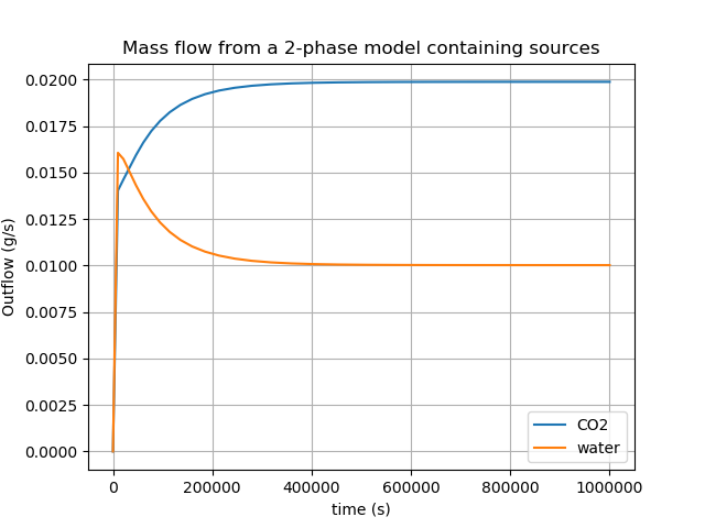
Figure 7: Mass flow rates from the two-phase model that contains a 0.01g/s source of water and a 0.02g/s source of gas, as well as PorousFlowOutflowBC boundary conditions that allow the fluids to freely exit the model.