Verification
In the context of large simulation codes solving nonlinear partial differential equation (PDE), verification involves quantifying numerical errors between known and discrete solutions (Oberkampf and Roy, 2010). Verification is composed of three components: Software Quality Assurance (SQA), code verification, and solution verification.
SQA is used to eliminate coding errors and is comprised primarily of software engineering practices: version control, regression testing, defect testing, quantification of code coverage, and code-to-code comparisons. Note that some literature includes SQA as a part of code verification (Oberkampf and Roy, 2010; Salari and Knupp, 2000).
Code verification ensures that the computer code is a faithful representation of the underlying mathematical model. This is achieved through the comparison of code solutions to a known solution as its mesh is refined. Through comparison to the expected behavior of the discretization error, it can be ensured that the numerical algorithm is behaving correctly.
Solution verification focuses on the estimation of numerical errors that occur when a mathematical model is discretized and solved on a digital computer. Though solution verification and code verification have some similar methodology, solution verification uses problems which do not have a known solution. Therefore, numerical errors must be estimated and not simply evaluated. This includes all sources of numerical error: round-off, statistical sampling, iterative error, and discretization errors.
"Verification must precede Validation.... Attempting to validate a model using a code that may still contain (serious) errors can lead to a false conclusion about the validity of the model" (Schwer, 2007). In other words, verification is a prerequisite to validation. Here, the two activities are distinguished to clearly separate testing of the numerical algorithm from other testing activities. Verification is concerned only with computer science and mathematics. Validation activities are concerned with the actual behavior of real-world systems and comparisons to experimental data. To that end, considerable emphasis has been placed on verification in BISON (Toptan et al., 2020).
Software Quality Assurance
"Often verification and validation are parts of an overarching software quality assurance (SQA) program. SQA methods are enacted to guide the software development cycle and may include recommendations or requirements for software engineering tasks such as gathering and recording customer requirements, using revision control software, writing code, testing the software, documenting the software, and releasing the application, among others. It is common to measure the quality of the software development process by assessing how well the development team is fulfilling the requirements in each of these areas" (Hales et al., 2014).
Version control
The BISON software is kept in a Enterprise GitHub version control repository at INL. The MOOSE software is open-source and maintained in a similar version control repository know as GitHub. The BISON unit and regression tests, example problems, validation cases and documentation are maintained in the same BISON Enterprise GitHub repository. This enables traceability of each code, validation case or documentation change. The author, date, and details of the changes are recorded with each commit to GitHub. It is also possible to retrieve a copy of the software from any point in its history. Through the use of revision control software, developers are able to maintain the current copy of BISON on their local machines and make frequent changes to BISON without fear of undoing another's changes or of making irrecoverable changes.
Software configuration management
The BISON team relies on software configuration management tools and practices set up for MOOSE applications. Continuous integration is also accomplished through Enterprise GitHub. With each commit to BISON (or any MOOSE-based component), Enterprise GitHub interfaces with the CIVET system and automatically compiles the software across multiple computer platforms. If the compilation process is successful, the new version of the software runs the complete set of regression tests. This also happens on multiple computer platforms. This continuous integration, as it is called, helps ensure that the regression tests run correctly at all times. If a commit causes a test to fail, the failure is immediately noted through an electronic message to the developers who then correct the error.
Defect testing
After the initial coding of the new changes, it is important to ensure that the new code capabilities function as expected, are free of coding mistakes, and dynamically tested to prevent regression. To address this part of SQA, three types of defect tests are used (Oberkampf and Roy, 2010; Toptan et al., 2018).
Unit tests verify the execution of a single function or subroutine and prove that the tested section of the code is free of mistakes.
Component tests compare a specific submodel or algorithm to expected output, showing that an overall model is running as expected.
System tests address the whole code, which indicates that a new model is properly integrated into the overall code structure.
In addition, a selection of the above tests is integrated into the BISON regression test suite and run periodically to ensure that code capabilities are not lost.
Regression testing
As a matter of engineering practice, BISON developers are responsible for developing regression tests for all of the code they develop. This helps ensure that future code changes do not break existing functionality. Some tests exercise the interaction of various models, and many others are single-feature verification tests.
Code coverage
In addition to the testing that occurs with each commit, code coverage data is also automatically produced. This information includes line and function coverage at the file, directory, and library level. The development team regularly reviews this information to ensure that the code coverage remains high.
All of this information (commit history and details, build status, test status, and code coverage) is available at the BISON GitHub site and is thus easily available to developers and others.
Documentation
As mentioned above, the BISON team maintains its documentation in the same Enterprise GitHub Repository that holds the application software. The documentation includes user instructions, theory, an assessment document, a publication list or bibliography, and a set of workshop or training presentation slides.
Code Verification
Code verification ensures that a model represented in computer code calculates the correct results as defined by the mathematical definition of the model. Verification is accomplished through tests, specially designed, that exercise a particular feature of a given model. As an example, for heat conduction, we can verify that the finite element solution of a linear temperature field is in fact linear even when the mesh is composed of irregular elements. For solid mechanics, we can test that the proper stress field results when a uniform pressure is applied.
By way of example, consider the process followed to introduce a new thermal conductivity model for UO fuel. Having identified the particular form of the model (the mathematical description), the developer can identify the inputs to the model (e.g., temperature) as well as the outputs (thermal conductivity). The developer creates a test that will exercise the new model. This test will require specific boundary conditions and perhaps other carefully controlled inputs in order to produce the exact results expected through an independent, analytic calculation.
The developer must of course also encode the relevant equations in the BISON software and compile the new code. Having done so, the developer exercises the new capability on the new test. If the computed thermal conductivity does not match the analytic expression, the developer searches for errors in the code and in the test until the discrepancy is resolved. Note that more than one verification test may be, and often is, required to give confidence that the encoded model is mathematically correct.
It should be understood that much of the underlying software in use by BISON has its own set of verification tests. In particular, verification tests concerned with the correctness of the finite element formulation are maintained at the MOOSE and libMesh levels.
BISON has many verification tests, checking solid mechanics, heat conduction, gap heat transfer, material models, mechanical contact, thermal contact, large strain capabilities, boundary conditions, plenum pressure determination, output, and many other phenomena needed for nuclear fuel analysis. That these tests run properly is evidence that the models have been implemented correctly. BISON SQA processes require that all new code committed to the repository is supported by adequate unit testing.
A review of several of BISON's verification tests, along with an overview of verification in the context of nuclear fuel performance software in general and of BISON in particular, is in Hales et al. (2014) and Toptan et al. (2020).
Method of exact and manufactured solutions
In general, the code verification process ensures that the coded numerical algorithm is a faithful representation of the underlying mathematical model. Here, we notate the the intended mathematical model as some nonlinear system operator .
(1)
The known solution is a function of space and time . The first option for finding a known solution is to use the method of exact solutions (MES) (Salari and Knupp, 2000), which involves calculating an exact analytical solution to Eq. (1). However, finding a nontrivial analytic solution to a complex nonlinear equation is difficult. The solution of these equations often requires significant simplifying assumptions. For example, many analytic solutions require that one or more of the terms in the PDE are trivial and eliminated from the solution. This process becomes even more difficult when a system of nonlinear equations is considered. Often, only approximate solutions are possible, for example, the well-known Navier-Stokes equations only have analytic solutions for the most trivial boundary and initial conditions.
A complete set of code verification analyses would require that all features of a code are tested. At its best, application of MES to the verification of all code options is a laborious process; at its worst, it can preclude sufficient testing of one or more relevant code options. For example, many analytic solutions involve only a single equation of state, varying property, or nonlinear source, and no solution is possible with multiple combinations of these complex physics. However, many codes default setting is to use a variety of equations of states, many varying properties, and nonlinear sources.
To address thorough code verification, analysts can employ the method of manufactured solutions (MMS) (Oberkampf and Roy, 2010; Roache, 1998; Salari and Knupp, 2000; McHale and others, 2009). In this method, a particular problem is worked backwards. The analyst determines a particular form of the solution . Then one seeks the necessary space- and time-dependent sources that would result in the manufactured solution:
The source is implemented in the simulation tool, then the verification process is performed. This methodology requires that the manufactured solution is formulated using continuous and smooth functions. These functions must be sufficiently complex to reveal nonlinearity in the governing equations. The chosen manufactured solution can be physically unrealistic, as it is intended only to test the underlying numerical algorithms. As with other verification methods, the observed order of accuracy should be consistent with the formal order.
Any necessary boundary conditions or initial conditions can be derived directly from the manufactured solution . Any equations of state, varying properties, or nonlinear sources can be incorporated into the MMS process by implementing them in the nonlinear operator . This allows all relevant code options to be tested in different combinations. In addition, MMS does not require the complex analytic solutions formed for MES, which greatly reduces the labor required for the verification process.
A series of traditional MES problems are solved for BISON to establish a pedigree. For the conduction solution, these include steady state problems solved on one- and two-dimensional domains with a variety of properties and external sources. Once this baseline pedigree is established, the MMS capability in BISON is demonstrated using a few manufactured problems (Toptan et al., 2020).
Solution Verification
Solution verification ensures that all validation simulations are adequately resolved in terms of spatial and temporal discretization, and all accompanying iterative solutions are sufficiently converged. This is a very large task given that the BISON validation cases are expected to number in the hundreds. Since many problems share similar geometry, materials and loading conditions, a first and substantial step will be to develop a representative problem for a given fuel type upon which solution verification is demonstrated. Some examples of this are given in Williamson et al. (2016) and Toptan et al. (2020).
Order of Accuracy
In this section, the formal order of accuracy is established for spatial and temporal discretization in BISON.
Spatial Order
To establish the spatial formal order of accuracy of the BISON solution algorithm, we provide a heuristic derivation (Burnett, 1987; Zienkiewicz et al., 2013) and point the reader to more mathematically rigorous analyses with the same result (Oliveira, 1968; Aziz, 1972; Oden and Reddy, 1976; Babuska and Szabo, 1982). In this work, the convergence of the computed solution to the analytical solution is analyzed as the size of the FE approaches zero, e.g., -convergence. No effort is made to quantify -convergence, during which convergence is analyzed as the order of the basis functions is increased (Babuska et al., 1981).
For the problems in this work, there are no singularities in mesh, properties, or external sources. All analytical solutions are continuous, smooth, and infinitely differentiable. The mesh has constant spacing and is uniformly refined. Under these conditions, the analysis of the discretization error is relatively simple. Here, we will analyze the error behavior of the quantity of interest (QoI) at some specified point in the domain , and use the results to generalize about the entire domain. First, note that the exact solution to a specific problem can be represented by a Taylor series about some point in the FE that contains :
(2)
This expansion assumes that is infinitely differentiable, which is true for all solutions in this work. Here, we have used a Taylor series approximation, which corresponds to a polynomial basis function of degree . Note that this procedure is equally applicable to other basis functions. The approximate solution calculated by the simulation tool using the chosen basis function of degree is
The Taylor series coefficients have been collapsed into the arbitrary constant . We define the length of an element as and note that because is a point inside the element. As the mesh is uniformly refined, , the approximate solution approaches arbitrarily close to the terms of Eq. (2) which are degree or lower. In addition, the domain point approaches the FE point as the mesh is refined. Therefore, the remaining terms of and greater will form the error at point .
Note that is a constant which includes the coefficient and derivative term from Eq. (2). For a sufficiently small , higher order terms become negligible and the term will dominate.
(3)
Now we generalize the point error in Eq. (3) using a norm over all space:
(4) where is an arbitrary constant that is problem-dependent, and the MOOSE function ElementL2Error is used to compute the norm over the domain :
As Eq. (4) is an exponential function, the slope of error on a log-log plot is the observed order of accuracy . Note that the finite element degree is sometimes referred to as the finite element order; however, it is not equivalent to the order of accuracy for a particular numerical method, which we notate as . Using two different meshes, the observed order of accuracy can be approximated as
(5)
All of the above arguments can also be applied to the flux. Since the flux is the first derivative of the QoI, its asymptotic rate should be one order lower than that of the function, that is its formal order is the same as the degree of the chosen FE.
where is an arbitrary constant that is problem-dependent, and the MOOSE function ElementH1SemiError is used to calculate the norm.
Here, and denote norms and semi-norms, respectively. The semi-norms behave mathematically as the norms do, except they can give zero values for non-zero inputs.
Eq. (5) can also be used to estimate the observed order of accuracy for the flux.
Temporal order
The MOOSE framework provides eight time discretization options which can be used to solve the transient BISON conservation equations: implicit/backward Euler (default), explicit/forward Euler, Crank-Nicolson, two-step backward differentiation formula (BDF), explicit midpoint, diagonally implicit Runge-Kutta (DIRK), explicit total variation diminishing (TVD) two-stage Runge-Kutta, and Newmark-beta.
Here, we derive the formal order of accuracy for the implicit Euler method, which is the default option in BISON. Similar exercises can be completed for all methods. We notate the transient conservation equation for some QoI as
where is some function of space , time , and the QoI which includes the finite element treatment of . The implicit Euler scheme discretizes this equation as
(6)
The QoI at is expanded about to approximate the numerical error in time:
This is substituted into Eq. (6) and simplified, yielding:
The second term scales with , the implicit Euler method is first order in time. Note that additional numerical error is introduced by the remaining terms, but these errors will be first order or greater. Similar analyses performed on the other time integration schemes would indicate that three of the methods (implicit Euler, explicit Euler, and explicit midpoint) are first order and the rest are second order.
Verification Procedure
The purpose of code verification is to ensure that discretized equations solved on a computation system faithfully represent the underlying continuous equations. This is achieved by comparing the formal and observed orders of accuracy. For each problem, a practical prescribed process is followed.
Define and solve the mathematical model. For MES problems, this involves selecting the conservation terms to be tested, setting boundary conditions and/or initial conditions, and mathematically solving the analytic problem. For MMS, a manufactured solution is chosen and the corresponding source terms derived.

Figure 1: FE types used in the BISON/MOOSE solution algorithm.
Choose the numerical algorithm and establish formal order of accuracy. In BISON, a variety of FE types (Figure 1) and temporal discretization schemes are available; one or more methods must be selected before solving the numerical problem.
Obtain numerical solutions. After formulating the required mesh and input, a numerical representation of the mathematical model is solved on at least four meshes. In this work, many meshes are evaluated to examine the behavior outside the asymptotic region. For steady state problems, only the spatial mesh is refined; however, the spatial and temporal mesh can be refined simultaneously for transient problems. Such combined order analysis methodology has been analyzed in Kamm et al. (2003).
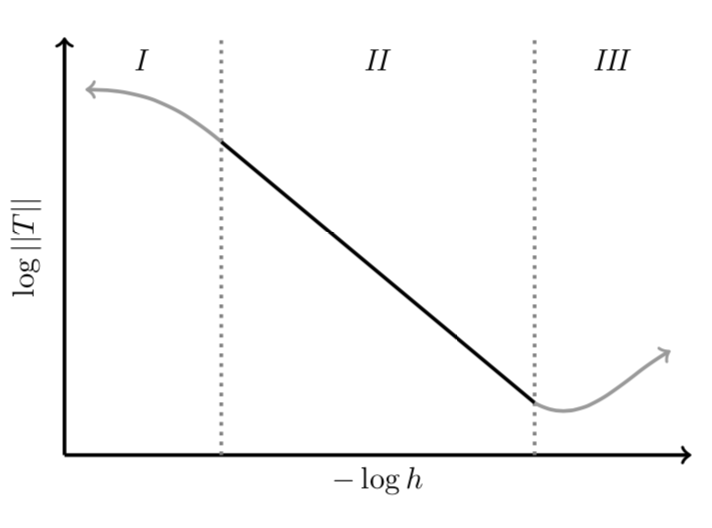
Figure 2: A pictorial representation of expected convergence behavior. Region I represents coarse meshes, region II is the asymptotic region, and region III is caused by round-off error.
Examine convergence behavior. The expected convergence behavior is shown in Figure 2 . When the mesh is coarse, higher order terms degrade the order of accuracy (region I). The region analyzed in the code verification process is the asymptotic region (region II), where the higher order terms are small enough that the observed order approximates the formal order. Finally, the numerical solution cannot converge to a tolerance finer than machine precision; therefore, as the mesh is refined further, there is a leveling-off of error and a slight increase as round-off error accumulates (region III). Finally, note that some problems will display hyper-convergent behavior. This is expected for problems where the FE order is high enough to exactly fit the analytic solution. For example, a first order method exactly approximates a linear solution and a second order method exactly approximates a quadratic solution. In these cases, the error plot starts in region III, as it immediately approximates the analytic solution to within numerical error.
Debug and correct errors if necessary. If the convergence behavior is significantly different than Figure 2, it indicates an error in the analytic solution, numerical model, or post-processing of the simulation results. Debugging and correcting these errors is an integral part of the verification process.
Document results. The numerical and analytic solutions will be plotted using different FE and meshes, then the convergence plot is created.
Once this process is complete and the observed order of accuracy matches the formal order of accuracy, the particular code verification problem is successful. The problem is added as evidence that the particular combination of physics, discretization, geometry, boundary conditions, and initial conditions is numerically free of coding mistakes.
Verification Problems
Contact
ECAR_131
ECAR_202
ECAR_5544
Mechanics
Other
TRISO_diffusion
Thermomechanics
thermal
References
- A K Aziz.
The Mathematical Foundations of The Finite Element Method with Applications to Partial Differential Equations.
Academic Press, New York, NY, 1972.[BibTeX]
- I Babuska and B Szabo.
On the rates of convergence of the finite element method.
Int J for Numerical Methods in Engineering, 18(3):323–341, 3 1982.
doi:10.1002/nme.1620180302.[BibTeX]
- I Babuska, B A Szabo, and I N Katz.
The $p$-version of the finite element method.
SAM J Numer Anal, 18(3):515–545, 6 1981.
doi:10.1137/0718033.[BibTeX]
- D S Burnett.
Finite Element Analysis from Concepts to Applications, chapter 9.
Addison-Wesley Publishing Company, Reading, MA, 1987.[BibTeX]
- E R de Arantes e Oliveira.
Theoretical foundations of the finite element method.
Int J Solids Struct, 4(10):929–952, 10 1968.
doi:10.1016/0020-7683(68)90014-0.[BibTeX]
- J.D. Hales, S.R. Novascone, B.W. Spencer, R.L. Williamson, G. Pastore, and D.M. Perez.
Verification of the BISON fuel performance code.
Annals of Nuclear Energy, 71:81–90, 2014.
doi:10.1016/j.anucene.2014.03.027.[BibTeX]
- J Kamm, W Rider, and J Brock.
Combined space and time convergence analysis of a compressible flow algorithm.
AIAA Paper, 2003.
doi:10.2514/6.2003-4241.[BibTeX]
- M P McHale and others.
Standard for verification and validation in computational fluid dynamics and heat transfer.
Standard ASME V&V 20-2009, American Society of Mechanical Engineers, 2009.[BibTeX]
- W L Oberkampf and C J Roy.
Verification and Validation in Scientific Computing.
Cambridge University Press, Cambridge, UK, first edition, 11 2010.[BibTeX]
- J T Oden and J N Reddy.
An Introduction to the Mathematical Theory of Finite Elements.
John Wiley & Sons, New York, NY, 1976.[BibTeX]
- P. J. Roache.
Verification and Validation in Computational Science and Engineering.
Hermosa Publishers, Albuquerque, NM, 1998.[BibTeX]
- K Salari and P Knupp.
Code verification by the method of manufactured solutions.
Technical Report SAND2000-1444, Sandia National Laboratories, 6 2000.
doi:10.2172/759450.[BibTeX]
- L. E. Schwer.
An overview of the PTC 60/V&V 10: guide for verification and validation in computational solid mechanics.
Engineering with Computers, 23:245–252, 2007.
doi:10.1007/s00366-007-0072-z.[BibTeX]
- A Toptan, N W Porter, J D Hales, R L Williamson, and M Pilch.
FY20 verification of BISON using analytic and manufactured solutions.
Technical Report CASL-U-2020-1939-000, CASL, March 2020.[BibTeX]
- A Toptan, N W Porter, R K Salko, and M N Avramova.
Implementation and assessment of wall friction models for LWR core analysis.
Annals of Nuclear Energy, 115:565–572, 2018.
doi:10.1016/j.anucene.2018.02.022.[BibTeX]
- R.L. Williamson, K.A. Gamble, D.M. Perez, S.R. Novascone, G. Pastore, R.J. Gardner, J.D. Hales, W. Liu, and A. Mai.
Validating the BISON fuel performance code to integral LWR experiments.
Nuclear Engineering and Design, 301:232–244, 2016.
doi:10.1016/j.nucengdes.2016.02.020.[BibTeX]
- O C Zienkiewicz, R L Taylor, and J Z Zhu.
The Finite Element Method Its Basis & Fundamentals.
Elsevier, New York, NY, 2013.
doi:10.1016/C2009-0-24909-9.[BibTeX]