Gap/Plenum Models
Gap Heat Transfer
Gap heat transfer is modeled using the relation, where is the total conductance across the gap, is the gas conductance, is the increased conductance due to solid-solid contact, and is the conductance due to radiant heat transfer.
Fill gas conductance
The fill gas conductance, is calculated for gap_geometry_type = PLATE, CYLINDER, and SPHERE (Toptan et al., 2019) as: (1) where is the fill gas thermal conductivity of the gas in the gap, corresponds to the gap size that is computed in the mechanics solution, is a roughness coefficient with as the surface roughness, and is the temperature jump distance for the surrounding solid bodies, . The gas temperature is computed as the arithmetic mean of the local temperatures of the surrounding surfaces. Note that the empirical coefficient, provides information regarding the fill gas conductance in the vicinity of surface irregularities and indirect information about contact for the closed gap configuration (Toptan et al., 2019).
Fill gas thermal conductivity
The thermal conductivity of a gas mixture, is generally a nonlinear function of mole fraction due to differences in polarity, molecular weight, or size of the constituents (Poling et al., 2000; Gray et al., 1970; Misic and Thodos, 1961). Lindsay and Bromley (1950) generalized the equation to calculate the multi-component mixture thermal conductivity . An expression was suggested for in terms of the thermal conductivities, the molecular weights, and inter-molecular potentials. Hirschfelder et al. (1954) indicated that the inter-molecular potentials are nearly unity. Later, Brokaw (1958) incorporated this assumption to simplify the expression. The resulting expression for the multi-component gas thermal conductivity is (2) with where is the number of constituents in the gas mixture, is the monatomic thermal conductivity of the constituent (Eq. (4)), and is the mole fraction of constituent.
Two modeling options are available in BISON to compute the fill gas thermal conductivity of each constituent, and its dependence on temperature and/or pressure, which are:
* DEFAULT, a temperature-dependent model from MATPRO (Allison et al., 1993)
* ADVANCED, a temperature and pressure-dependent model from Toptan et al. (2019)
DEFAULT
The thermal conductivity of the constituent, is computed from MATPRO (Allison et al., 1993) for ten gases (e.g., helium, argon, krypton, xenon, hydrogen, nitrogen, oxygen, carbon monoxide, carbon dioxide, and water vapor). The emprical coefficients were derived based on the experimental data by Gandhi and Saxena (1968). Note that the thermal conductivity of neon was not provided in MATPRO, an expression was derived herein for neon using the data by Gandhi and Saxena (1968). The formulation is provided in the following form: (3) where and are the empirical coefficients that are tabulated in Table 1, and is the temperature in K. Note that the empirical coefficients of the MATPRO model for monatomic inert gases were calibrated based on the data by Gandhi and Saxena (1968), therefore, the model is considered valid up to 520C. Additionally, thermal conductivity of neon, argon, and xenon at high gas temperatures is given by Springer and Wingeier (1973) above 1000 K in the form of Eq. (3). The empirical coefficients are provided in Table 1.
Table 1: Empirical coefficients and for Eq. (3).
| Gas type | Applicability | Reference | ||
|---|---|---|---|---|
| helium | 2.639 | 0.7085 | 73–793 K | Allison et al. (1993) |
| neon | 9.000 | 0.691 | 73–793 K | |
| 9.683 | 0.685 | 1000–1500 K | Springer and Wingeier (1973) | |
| argon | 2.986 | 0.7224 | 73–793 K | Allison et al. (1993) |
| 4.905 | 0.651 | 1000–2500 K | Springer and Wingeier (1973) | |
| krypton | 8.247 | 0.8363 | 173–793 K | Allison et al. (1993) |
| xenon | 4.351 | 0.8616 | 173–793 K | Allison et al. (1993) |
| 1.140 | 0.710 | 1000–1500 K | Springer and Wingeier (1973) | |
| hydrogen | 1.097 | 0.8785 | Allison et al. (1993) | |
| nitrogen | 5.314 | 0.6898 | Allison et al. (1993) | |
| oxygen | 1.853 | 0.8729 | Allison et al. (1993) | |
| carbon monoxide | 1.403 | 0.9090 | Allison et al. (1993) | |
| carbon dioxide | 9.460 | 1.3120 | Allison et al. (1993) |
Figure 1 shows the fill gas thermal conductivity predictions for the selected inert gases. The MATPRO model predictions agree well with the model predictions using the relations from Springer and Wingeier (1973). For this reason, the relations by Springer and Wingeier (1973) are not implemented into the code.
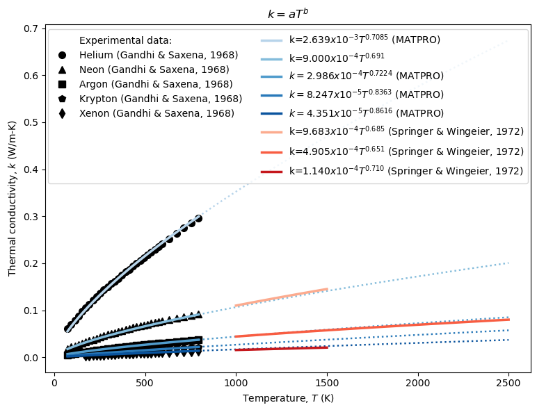
Figure 1: The fill gas thermal conductivity for the selected inert gases. MATPRO model predictions are presented by the blue solid lines at corresponding applicability ranges, while MATPRO model predictions at extended temperature ranges are presented by the blue dashed lines. Experimental data from Gandhi and Saxena (1968) are shown with the markers. Red solid lines represent the model predictions using relations from Springer and Wingeier (1973) for neon, argon, and xenon at high gas temperatures (1000–2500 K).
For water vapor, the fill gas thermal conductivity is calculated as follows: where is the gas temperature in C.
ADVANCED
The above correlation is only temperature-dependent and is calibrated to experimental data at pressures below 0.1 MPa (Gandhi and Saxena, 1968). The thermal conductivity of all gases increases with pressure, though the extent of this dependence varies depending upon the pressure (see Figure 2). Three distinct pressure regions exist (Toptan et al., 2019):
a very low-pressure zone (below 0.1 kPa), the Knudsen domain in which the thermal conductivity is almost proportional to pressure,
a low-pressure zone (below 1.0 MPa) in which the pressure dependence is generally neglected because of its insignificant contribution, and
a high-pressure zone (above 1.0 MPa) in which increasing pressure increases the thermal conductivity.
To account for the pressure dependence that is embedded in the density term, the thermal conductivity is expressed by Tournier and El-Genk (2008) as:
(4) where where is the thermal conductivity of pure dilute gases based on the kinetic theory, is the dynamic viscosity of pure dilute gases, is the pseudo-critical thermal conductivity, is the characteristic molar volume, is the excess thermal conductivity, is molecular weight, and is the reduced density.
Table 2: Critical gas properties are from Tournier and El-Genk (2008).
| helium | neon | argon | krypton | xenon | |
|---|---|---|---|---|---|
| (g/mol) | 4.003 | 20.180 | 39.948 | 83.798 | 131.293 |
| (MPa) | 0.2275 | 2.678 | 4.863 | 5.51 | 5.84 |
| (K) | 5.2 | 44.5 | 150.69 | 209.4 | 289.7 |
| (kg/m) | 69.64 | 481.9 | 535.6 | 908.4 | 1110.0 |
| 3.063 | 8.4528 | 6.989 | 6.963 | 7.568 | |
| (K) | -21.33 | 16.47 | 65.70 | 71.07 | 112.31 |
| 0.724 | 0.643 | 0.640 | 0.667 | 0.655 |
The reduced-state plot of thermal conductivity for the selected inert gases is obtained following the approach developed by Owens and Thodos (1957). Reduced thermal conductivities are calculated using Eq. (4) and plotted against the reduced temperatures on a log-log plot in Figure 2.
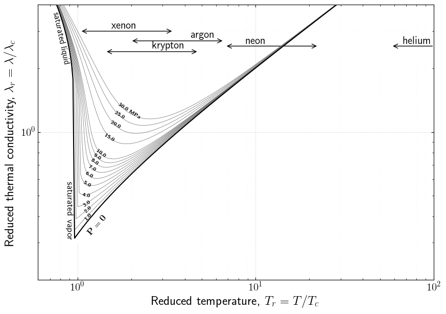
Figure 2: The reduced-state plot of thermal conductivity for the selected inert gases Toptan et al. (2019). Arrows represent the gas temperature from 300K to 1000K.
Gas Density
The behavior of a fluid deviates from that of an ideal gas as its density increases. Many corrections are introduced in the literature, which lead to the virial expansion form of the ideal gas law in terms of the macroscopic thermodynamic properties and particle interactions. The virial equation of state (Onnes, 1901; Mason and Spurling, 1969) is expressed as Eq. (5). If the gas temperature and pressure are known, the density of the gas is computed by solving the cubic equation given in Eq. (5), and the density is obtained by employing a root-finding algorithm. Since it is a cubic equation, there may be three possible solutions. The highest real value is assigned for the gas molar density. Note that the gas density is only calculated when the ADVANCED option is selected for the fill gas thermal conductivity.
(5) where is pressure (Pa), is temperature (K), is ideal gas constant (8.314 J/mol-K), is compressibility factor, is molar density, is the i-th virial coefficient that is only a function of temperature (see Figure 3).
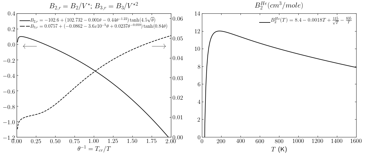
Figure 3: Left plot: the reduced second and third virial coefficients, and , versus the reduced temperature, , for Xe, Kr, Ar and Ne; right plot: the second virial coefficient for He as a function of temperature, where its third virial coefficient is neglected due to its dilute gas behavior. Note that the closure relations are calibrated by Tournier and El-Genk (2008).
Temperature jump distance
The difference between the wall temperature and gas temperature at the wall is known as the temperature jump condition. Poisson proposed the discontinuity in temperature as where is the wall temperature and is the temperature continued without change right up to the wall itself. Later, Kennard calculated the proportionality constant by equating the excess energy carried by the incident stream to the total heat conducted across a parallel plane out in the gas.
Two modeling options are available in BISON to compute the temperature jump distance, and its dependence on the gas properties, which are:
* LANNING, Kennard's model based on a review by Lanning and Hann (1975), and
* TOPTAN, Kennard's model based on a review by Toptan et al. (2019).
LANNING
Temperature jump distance is calculated using Kennard's model based on a review by Lanning and Hann (1975). where the units of , , and are , , and respectively, is mole fraction of i-th gas species, is molcular weight of i-th gas species, and is accommodation coefficient for the gas mixture.
TOPTAN
Kennard's expression (Kennard, 1938) for the temperature jump distance, for gap_geometry_type = PLATE, CYLINDER, and SPHERE is calculated based on a review by Toptan et al. (2019): (6) with
In the code, it is applied as follows: for similar surfaces (i.e., ). The Kennard coefficient becomes See Toptan et al. (2019) and Toptan et al. (2020) for more detailed information.
Thermal accommodation coefficient
The accommodation coefficient is a measure of the interaction at a gas-solid interface and indicates the degree to which molecules are accommodated to the surface. Knudsen (1911) introduced the accommodation coefficient and prefered to attach a temperature to each of these streams of molecules as where is the thermal accommodation coefficient, is the reflection temperature, is the incident temperature, and is the wall tempearture .
Two modeling options are available in BISON to compute the thermal accommodation coefficient, and its dependence on the gas properties, which are:
* DEFAULT, a model from MATPRO (Allison et al., 1993) based on Lanning and Hann (1975), and
* TOPTAN, a model that is recommended by Toptan et al. (2019).
DEFAULT
The accomodation coefficients for helium and xenon are calculated as: (7) (8) For a gas mixture, (9) where is molecular weight of xenon, is molecular weight of helium, and is molecular weight of gas mixture.
TOPTAN
Baule (1914) proposed a closed-form expression for considering interactions between two hard spheres. The first is an incident gas atom, and the other is an initially stationary solid atom. Under these assumptions, the accommodation coefficient is . There exist many models available in the literature; however, the Goodman and Wachman (1967) formula is widely used. Toptan et al. (2019) altered the formulation as Eq. (10), calibrated with the literature data for interactions between selected monatomic inert gases and typical engineering surfaces. Note that the mass of the solid is set to a very large value (i.e., g/mol) in the calibration. (10) where is the molecular weight of the incident gas, is the molecular weight of the stationary solid, is the coefficient matrix Table 3, , and is the ratio of the molecular weights.
Table 3: The thermal accommodation coefficient of the selected inert gases using Eq. (10) with the coefficient matrix, for a variety of gases (Toptan et al., 2019).
| helium | neon | argon | krypton | xenon | |
|---|---|---|---|---|---|
| -1.055 | -0.611 | 0.032 | 0.344 | 0.784 | |
| 146.7 | 360.6 | 591.3 | 724.7 | 916.7 |
Mikami et al. (1966) expressed the thermal accommodation coefficient of a gas mixture from the energy balance as (11) where the summation is over each component of the mixture.
Thermal Contact Conductance
When there is partial or complete contact between two solid bodies, an additional heat transfer term is necessary. The resistance at the interface is called constriction (or contact) resistance, and is defined as (12) where is the heat flow rate, is the temperature drop required to overcome the thermal resistance at the contact, and is the apparent area.
Initially, Kottler (1927) used the classical electrical analogy to solve the constriction resistance in an electrical conductor exhibiting a discontinuous reduction in cross-section. Maxwell (1954) indicated that the temperature difference plays the same role in the flow of heat as the electrical potential does in the theory of electric current; therefore, thermal resistances may be expressed mathematically in the same manner as electrical resistances, except that electrical resistivity is equivalent to the reciprocal of thermal conductivity. Holm (1958) extended the work of Kottler and solved the thermal constriction resistance for an isothermal circular contact area with a radius on a flat surface of a semi-infinite body as and the total constriction resistance of two similar semi-infinite bodies as . Clark and Powell (1962) derived the total constriction resistance of two dissimilar semi-infinite bodies over a circular area as (13)
If the idealized contact geometry is assumed, the total parallel resistance of solid contacts in a particular region can be approximated as (Clausing and Chao, 1965). With the approximated constriction resistance the contact conductance can be estimated once the apparent area is known.
Archard expressed the contact area when the deformation is truly elastic as , where is a constant depending upon the local radius of curvature and elastic constants of the materials. Analogously, Archard correlated the contact area as where is the flow pressure of hardness of the softer material when the asperities are performed deformed plastically (Archard, 1953; Archard, 1957). The relationship between the apparent area and the contact area can be generalized to the form of (14) where is the load on the contact interface (i.e., contact pressure), is Meyer's hardness of the softer material, and is the index of departure from elastic deformation (e.g., for elastic, for plastic).
As indicated by Bowden and Tabor (1950), a plastic deformation mechanism is postulated since the real area of contact is nearly proportional to the load for all types and shapes of practical surface irregularities. This is the reason why early thermal contact models (Cetinkale and Fishenden, 1951; Boeschoten and Held, 1957; Fenech and Rohsenow, 1959; Laming, 1961; Cooper et al., 1969) in the literature assumed this model function form. Thus, inserting the total contact area (i.e., ) in Eq. (14) yields (15)
Determination of contact shapes, deformation of surface irregularities, or the number of contact spots is neither known nor accurately measurable. Due to the difficulty of determining these quantities, approximated gap closure relations are used in nuclear fuel performance modeling. The Ross-Stoute model (Ross and Stoute, 1962) is a common solid contact model where is introduced into the correlation as a function of the surface roughness . The default model in BISON is a modified version of the correlation suggested by Ross and Stoute (1962): (16) where is an empirical constant, and are the thermal conductivities of the solid materials in contact, is the contact pressure, is the average gas film thickness (approximated as 0.8(), and is the Meyer hardness of the softer material (i.e., the cladding). From measurements on steel in contact with aluminum, Ross and Stoute (1962) recommend = 10 , which is the default value in BISON. The default value of the Meyer hardness is 680MN/m. Alternatively, the following temperature-dependent correlation (Hagrman et al., 1980) is available in the code.
As an option, the chemical interaction layer at the fuel-cladding interface can be taken into account in the contact term. Based on experimental work (Kim, 2010), the growth of a (U,Zr)O layer is considered during fuel-cladding contact and is described based on a parabolic law (17) where (m) is the layer thickness, and (Kim, 2010) is the parabolic growth rate. Eq. (17) is solved numerically by where is the layer thickness at the current time step (m), is the layer thickness at the previous time step (m), and is the time increment (s).
The chemical interaction layer is assumed to fill the fuel and cladding roughnesses according to its thickness, effectively reducing the and terms in Eq. (16) and improving the heat transfer.
Conductance due to radiant heat transfer
The heat transfer due to thermal radiation is calculated using the expression of Bird et al. (1960)—which assumes two infinite parallel gray surfaces, where radiation leaving the first body and is directly intercepted by the second body—as where is the Stefan-Boltzmann constant (5.67 W/mK), is an emissivity function, and and are the temperatures of the radiating surfaces. The radiant conductance is thus approximated which reduces to For infinite parallel plates, the emissivity function is defined as where and are the emissivities of the radiating surfaces. This is the specific function implemented in BISON.
Mechanical Contact
Mechanical contact between fuel pellets and the inside surface of the cladding is based on three requirements: That is, the penetration distance (typically referred to as the gap in the contact literature) of one body into another must not be positive; the contact force opposing penetration must be positive in the normal direction; and either the penetration distance or the contact force must be zero at all times.
In BISON, these contact constraints are enforced through the use of node/face constraints. Specifically, the nodes of the fuel pellets are prevented from penetrating cladding faces. This is accomplished in a manner similar to that detailed by Heinstein and Laursen (1999). First, a geometric search determines which fuel pellet nodes have penetrated cladding faces. For those nodes, the internal force computed by the divergence of stress is moved to the appropriate cladding face at the point of contact. Those forces are distributed to cladding nodes by employing the finite element shape functions. Additionally, the pellet nodes are constrained to remain on the pellet faces, preventing penetration. BISON supports frictionless and tied contact. Friction is an important capability, and preliminary support for frictional contact is available.
Finite element contact is notoriously difficult to make efficient and robust in three dimensions. That being the case, effort is underway to improve the contact algorithm.
Gap/plenum pressure
The pressure in the gap and plenum is computed based on the ideal gas law, (18) where is the gap/plenum pressure, is the moles of gas, is the ideal gas constant, is the temperature, and is the volume of the cavity. The moles of gas, the temperature, and the cavity volume in this equation are free to change with time. The moles of gas at any time is the original amount of gas (computed based on original pressure, temperature, and volume) plus the amount in the cavity due to fission gas released. The temperature is taken as the average temperature of the pellet exterior and cladding interior surfaces, though any other measure of temperature could be used. The cavity volume is computed as needed based on the evolving pellet and clad geometry.
There is an option to specify additional, unmeshed volumes with corresponding temperatures that communicate directly with the cavity. In this case the pressure becomes:
where is the number of additional volumes. If simulation past cladding rupture is desired the plenum pressure is set equal to the equilibrium pressure defined by the user.
Gap/plenum temperature
The gap/plenum pressure (see above section) requires the temperature of the gas inside the cladding. Many choices are possible when supplying this temperature. It may be appropriate to supply the temperature at a node, the average temperature of several nodes, or data from an experiment. In this section, we outline an approach for calculating an average gas temperature that takes into account the entire fuel/cladding system.
We seek a weighted average temperature that accounts for the fact that the majority of the gas is in the plenum region. Using a volume-weighted average, the average gas temperature can be approximated as where is the temperature at a point in the gap/plenum and is the volume occupied by the gas. It is necessary to make some approximations in the calculation of this temperature since the gap and plenum volumes are not meshed. We assume that a differential volume () is equal to a varying distance times a differential area (). This change is appropriate for replacing the integral over the volume of an enclosed space with the integral of the medial surface of that space times a distance representing the depth of the volume at a particular point on the surface.
With this change, it is necessary to replace with the temperature associated with . We take this temperature to be the average temperature of the outer and inner surfaces bounding the volume: The medial surface of the gas volume is not known. We instead use the fuel surface. This gives where is the fuel surface, is the temperature across the gap, is the temperature on the fuel surface, and is the gap distance. This approximation is a good one for the plenum region since the plenum volume can be accurately calculated given our assumptions. The accuracy of the calculation will be lower for the gap volume contribution, but since this volume is small (zero in areas of fuel/cladding contact) it is less important.
Note that since this approach places an appropriately large weight on the gas in the plenum, it is important that the temperature of the fuel adjacent to the plenum be accurate. It may be necessary to place insulating pellets in a model in order to calculate realistic temperatures at the top of the fuel stack.
Integral Fuel Burnable Absorber (IFBA)
An integral fuel burnable absorber (IFBA) is used for optimizing fuel assembly reactivity and power distribution in a core. The IFBA is usually applied as a thin layer of over some length of a fuel rod. Since the IFBA layer is normally on the order of a few microns thick, the helium atoms generated are assumed to be released immediately into the plenum. In addition, the IFBA layer is depleted very quickly and is typically used up in the first of burnup or months of exposure.
Two models for the helium gas production (i.e., boron-10 depletion) have been implemented in BISON. These models are discussion on the IFBAHeProduction documentation page in detail.
References
- C. M. Allison, G. A. Berna, R. Chambers, E. W. Coryell, K. L. Davis, D. L. Hagrman, D. T. Hagrman, N. L. Hampton, J. K. Hohorst, R. E. Mason, M. L. McComas, K. A. McNeil, R. L. Miller, C. S. Olsen, G. A. Reymann, and L. J. Siefken.
SCDAP/RELAP5/MOD3.1 code manual, volume IV: MATPRO-A library of materials properties for light-water-reactor accident analysis.
Technical Report NUREG/CR-6150, EGG-2720, Idaho National Engineering Laboratory, 1993.[BibTeX]
- J. F. Archard.
Elastic deformation and the contact of surfaces.
Nature, 172:918 – 919, 11 1953.
doi:10.1038/172918a0.[BibTeX]
- J. F. Archard.
Elastic deformation and the laws of friction.
Proceedings of the Royal Society of London, Series A, Mathematical and Physical Sciences, 243(1233):190–205, 12 1957.
URL: http://www.jstor.org/stable/100445.[BibTeX]
- B Baule.
Theoretische behandlung der erscheinungen in verdünnten gasen.
Annalen der Physik, 349(9):145–176, 1914.
doi:10.1002/andp.19143490908.[BibTeX]
- R. B. Bird, W. E. Stewart, and E. N. Lightfoot.
Transport Phenomena.
John Wiley & Sons, Inc., New York, 1960.[BibTeX]
- F. Boeschoten and E. Van der Held.
The thermal conductance of contacts between aluminum and other metals.
Physica, 23:37–44, 1957.
doi:10.1016/S0031-8914(57)90236-7.[BibTeX]
- F. P. Bowden and D. Tabor.
The Friction and Lubrication of Solids.
Oxford University Press, New York, 1950.[BibTeX]
- R. S. Brokaw.
Approximate formulas for the viscosity and thermal conductivity of gas mixtures.
Chemical Physics, 29(2):391–397, 1958.
doi:10.1063/1.1744491.[BibTeX]
- T. N. Cetinkale and M. Fishenden.
Thermal conductance of metal surfaces in contact.
In General Discussion on Heat Transfer, 271–275. Conf. of Inst. of Mech. Eng. and ASME, September 1951.[BibTeX]
- W. T. Clark and R. W. Powell.
Measurement of thermal conduction by the thermal comparator.
Scientific Instruments, 39(11):545–551, 1962.
doi:10.1088/0950-7671/39/11/303.[BibTeX]
- A. M. Clausing and B. T. Chao.
Thermal contact resistance in a vacuum environment.
Heat Transfer, 87(2):243–250, May 1965.
doi:10.1115/1.3689082.[BibTeX]
- M. G. Cooper, B. B. Mikic, and M. M. Yovanovich.
Thermal contact conductance.
Int. J. Heat and Mass Transfer, 12:279–300, 3 1969.
doi:10.1016/0017-9310(69)90011-8.[BibTeX]
- H Fenech and W M Rohsenow.
Thermal Conductance of Metal Surfaces in Contact.
USAEC Report NYO-2136, Massachusetts Inst. of Tech., Cambridge. Heat Transfer Lab., 1959.[BibTeX]
- J. M. Gandhi and S. C. Saxena.
Correlated thermal conductivity data of rare gases and their binary mixts. at ordinary pressures.
Chemical & Engineering Data, 13(3):357–361, 07 1968.
doi:10.1021/je60038a016.[BibTeX]
- F O Goodman and H Y Wachman.
Formula for thermal accommodation coefficients.
Chemical Physics, 46(6):2376–2386, 1967.
doi:10.1063/1.1841046.[BibTeX]
- P Gray, S Holland, and A O S Maczek.
Thermal conductivities of binary mixtures of organic vapours and inert diluents.
Trans Fraday Society, 66:107, 1970.
doi:10.1039/TF9706600107.[BibTeX]
- D L Hagrman, G A Reymann, and R E Manson.
MATPRO-Version 11 (rev. 1): A Handbook of Materials Properties for Use in the Analysis of Light Water Reactor Fuel Rod Behavior.
USNRC Report NUREG/CR-0497, TREE-1290, Idaho National Engineering Laboratories, February 1980.
doi:10.2172/6442256.[BibTeX]
- M. Heinstein and T. Laursen.
An algorithm for the matrix-free solution of quasistatic frictional contact problems.
International Journal for Numerical Methods in Engineering, 44(9):1205–1226, 1999.
doi:10.1002/(SICI)1097-0207(19990330)44:9<1205::AID-NME550>3.0.CO;2-0.[BibTeX]
- J O Hirschfelder, C F Curtiss, and R B Bird.
Molecular Theory of Gases and Liquids.
John Wiley and Sons, Inc., New York, 1954.[BibTeX]
- R. Holm.
Electrical Contacts Handbook.
Springer Verlag, Berlin, 1958.[BibTeX]
- E. H. Kennard.
Kinetic Theory of Gases, with an Introduction to Statistical Mechanics.
McGraw-Hill Book Company, inc., New York, London, 1938.[BibTeX]
- K.-T. Kim.
UO$_2$/Zry-4 chemical interaction layers for intact and leak PWR fuel rods.
Journal of Nuclear Materials, 404(2):128–137, 2010.
doi:10.1016/j.jnucmat.2010.07.013.[BibTeX]
- M. Knudsen.
Die molekulare wärmeleitung der gase und der akkommodationskoeffizient.
Annalen Der Physik, 34(4):593–656, 1911.
doi:10.1002/andp.19113390402.[BibTeX]
- F. Kottler.
Elektrostatik der leiter.
Theorien der Elektrizität Elektrostatik, 12:472–473, 1927.
doi:10.1007/978-3-642-99428-9_4.[BibTeX]
- L. C. Laming.
Thermal conductance of machined metal contacts.
In ASME International Heat Transfer Conference, volume I, 65–76. Boulder, Colorado, September 1961.[BibTeX]
- D. D. Lanning and C. R. Hann.
Review of methods applicable to the calculation of gap conductance in zircaloy-clad uo2 fuel rods.
Technical Report BWNL-1894, UC-78B, Pacific Northwest National Laboratory, 1975.[BibTeX]
- A. L. Lindsay and L. A. Bromley.
Thermal conductivity of gas mixtures.
Industrial and Engineering Chemistry, 42(8):1508–1511, 1950.
doi:10.1021/ie50488a017.[BibTeX]
- E A Mason and T H Spurling.
The Virial Equation of State.
Toronto, Pergamon Press, 1969.[BibTeX]
- J.C. Maxwell.
Treatise on Electricity and Magnetism, Vol. 1.
Dover Publications, 1954.[BibTeX]
- H Mikami, Y Endo, and Y Takashima.
Heat transfer from a sphere to rarefied gas mixtures.
Int J Heat and Mass Transfer, 9(12):1435–1448, 1966.
doi:10.1016/0017-9310(66)90139-6.[BibTeX]
- D Misic and G Thodos.
The thermal conductivity of hydrocarbon gases at normal pressures.
J AIChE, 7(2):264, 1961.
doi:10.1002/aic.690070219.[BibTeX]
- H K Onnes.
Expression of the Equation of State of Gases and Liquids by Means of Series.
Koninklijke Nederlandse Akademie van Wetenschappen Proceedings Series B Physical Sciences, 4:125–147, 1901.[BibTeX]
- E J Owens and G Thodos.
Thermal-conductivity-reduced-state Correlation for the Inert Gases.
AIChE, 3(4):454–461, 1957.
doi:10.1002/aic.690030407.[BibTeX]
- B E Poling, J M Prausnitz, and J P O'Connell.
The Properties of Gases and Liquids.
McGraw-Hill, 5 edition, 2000.
ISBN 0-07-011682-2.[BibTeX]
- A. M. Ross and R. L. Stoute.
Heat transfer coefficient between UO$_2$ and Zircaloy-2.
Technical Report AECL-1552, Atomic Energy of Canada Limited, 1962.[BibTeX]
- G. S. Springer and E. W. Wingeier.
Thermal conductivity of neon, argon, and xenon at high temperatures.
The Journal of Chemical Physics, 59(5):2747–2750, 1973.
doi:10.1063/1.1680394.[BibTeX]
- A Toptan, D J Kropaczek, and M N Avramova.
Gap conductance modeling II: optimized model for UO$_2$-zircaloy interfaces.
Nuclear Engineering and Design, 355:110289, 2019.
doi:10.1016/j.nucengdes.110289.[BibTeX]
- A Toptan, D J Kropaczek, and M N Avramova.
Gap conductance modeling I: theoretical considerations for single- and multi-component gases in curvilinear coordinates.
Nuclear Engineering and Design, 353:110283, 2019.
doi:10.1016/j.nucengdes.2019.110283.[BibTeX]
- A Toptan, D J Kropaczek, and M N Avramova.
On the validity of the dilute gas assumption for gap conductance calculations in nuclear fuel performance codes.
Nuclear Engineering and Design, 350:1–8, 2019.
doi:10.1016/j.nucengdes.2019.04.042.[BibTeX]
- Aysenur Toptan, Jason D. Hales, Richard L. Williamson, Stephen R. Novascone, Giovanni Pastore, and David J. Kropaczek.
Modeling of gap conductance for LWR fuel rods applied in the BISON code.
Journal of Nuclear Science and Technology, 57(8):963–974, 2020.
doi:10.1080/00223131.2020.1740808.[BibTeX]
- J-M P Tournier and M S El-Genk.
Properties of noble gases and binary mixtures for closed brayton cycle applications.
Energy Conversion and Management, 49(3):469–492, 2008.
doi:10.1016/j.enconman.2007.06.050.[BibTeX]