MOOSE Workshop
July 2026
Idaho National Laboratory
www.inl.gov
Established in 2005, INL is the lead nuclear energy R&D laboratory for the Department of Energy
"Establish a world-class capability in the modeling and simulation of advanced energy systems..."
INL is the one of the largest employers in Idaho with over 6,000 employees and 500 interns
In 2024 the INL budget was over $2 billion
INL is the site where 52 nuclear reactors were designed and constructed, including the first reactor to generate usable amounts of electricity: Experimental Breeder Reactor I (EBR-1)

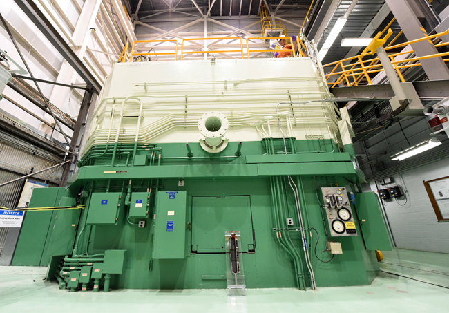
Advanced Test Reactor (ATR)
World's most powerful test reactor (250 MW thermal)
Constructed in 1967
Volume of 1.4 cubic meters, with 43 kg of uranium, and operates at 60C

Transient Reactor Test Facility (TREAT)
TREAT is a test facility specifically designed to evaluate the response of fuels and materials to accident conditions
High-intensity (20 GW), short-duration (80 ms) neutron pulses for severe accident testing
National Reactor Innovation Center (NRIC)
NRIC is composed of two physical test beds to build prototypes of advanced nuclear reactors:
DOME (Demonstration of Microreactor Experiments) in the historic EBR-II facility, a test bed site capable of hosting operational nuclear reactor concepts that produce less than 20MW thermal power.
LOTUS (Laboratory for Operation and Testing in the U.S.) in the historic Zero Power Physics Reactor (ZPPR) Cell, a test bed site capable of hosting operational nuclear reactor concepts that produce less than 500kW thermal power.
NRIC also manages the open-source Virtual Test Bed to demonstrate advanced reactors through modeling and simulation. More information about NRIC can be found at https://nric.inl.gov.
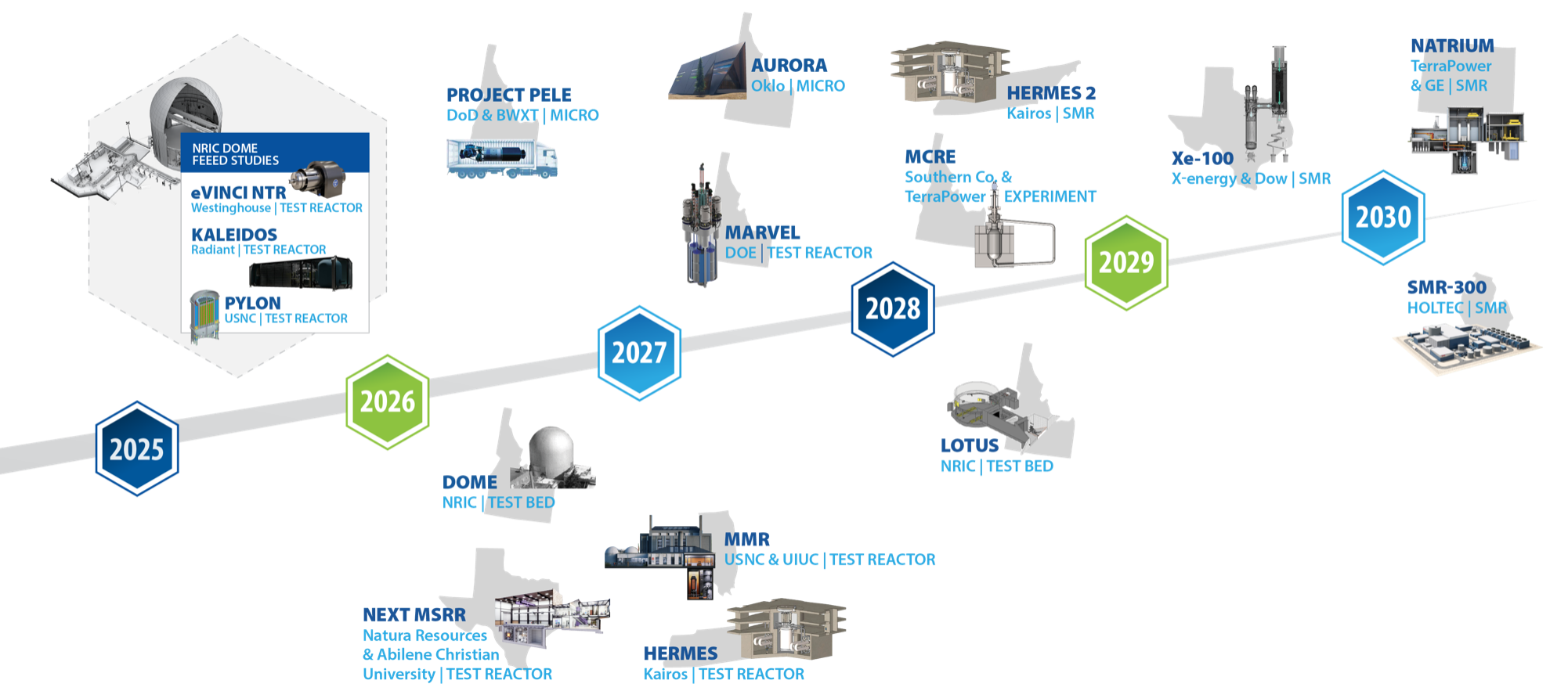
Advanced Reactor Demonstration Timeline
MOOSE
Multi-physics Object Oriented Simulation Environment
mooseframework.inl.gov

History and Purpose
Development started in 2008
Open-sourced in 2014
Designed to solve computational engineering problems and reduce the expense and time required to develop new applications by:
Being easily extended and maintained
Working efficiently on a few and many processors
Providing an object-oriented, extensible system for creating all aspects of a simulation tool
Motivated by multiphysics problems in nuclear engineering, but applications have extended into diverse fields
Core team at Idaho National Laboratory, but with significant contributions from other laboratories, universities, and industry, both domestically and internationally
By The Numbers
250 contributors
58,000 commits
5,000 unique visitors per month
~40 new Discussion participants per week
150M tests per week
General Capabilities
Continuous and Discontinuous Galerkin FEM
Finite Volume
Supports fully coupled or segregated systems, fully implicit and explicit time integration
Automatic differentiation (AD)
Unstructured mesh with FEM shapes
Higher order geometry
Mesh adaptivity (refinement and coarsening)
Massively parallel (MPI and threads)
User code agnostic of dimension, parallelism, shape functions, etc.
Native support for executing multiphysics simulations across applications
GPU support for execution via MFEM and Kokkos
Operating Systems:
macOS (Conda, Docker)
Linux (Apptainer, Conda, Docker)
Windows (Docker, WSL)
Object-oriented, pluggable system

Example Code
Software Quality
Follows a Nuclear Quality Assurance Level 1 (NQA-1) development process
All changes undergo independent review and must pass regression tests before merge
Includes a test suite and documentation system to allow for agile development while maintaining a NQA-1 process
External contributions are guided through the process by the team, and are very welcome!
Development Process

Community
github.com/idaholab/moose/discussions

License
LGPL 2.1
Does not limit what you can do with your application
Can license/sell your application as closed source
Modifications to the library itself (or the modules) are open source
New contributions are automatically LGPL 2.1
Multiphysics Simulation
Historical Multiphysics Simulation
Predictive multiphysics capability involved best-estimate calculations
Best estimates: data and correlation driven, many approximations
Necessitated experimental data for each design
Physics performed independently
Was a "siloed" task; handoffs of data/results from person to person
While individual codes were computationally efficient and well validated, coupling them was neither efficient nor well validated
Used many approximations for evaluations of safety parameters
Pin-power reconstruction, gap conductance, spacer grid models
Modern Multiphysics Simulation
Direct, physics-based models of all components
Reduces approximations as needed
Can be computationally expensive
Can employ tighter and more consistent coupling
Length and time scales of physics can be vastly different
What does this change for the analyst?
Not as well validated:
Experiments prohibitively expensive
Very large design space
Modularity is Key
Data should be accessed through strict interfaces with code having separation of responsibilities
Allows for "decoupling" of code
Leads to more reuse and less bugs
Challenging for FEM
Shape functions, degrees of freedom, meshing, quadrature points, material properties, analytic functions, global integrals, data transfer, ...
The complexity makes computational science codes brittle and hard to reuse
A consistent set of "systems" are needed to carry out common actions, these systems should be separated by interfaces
Finite-Element Reactor Fuel Simulation
MOOSE Coupling Strategies
Coupling strategies:
Full coupling: Solve all physics in a single (linear or nonlinear) system
Loose coupling: Solve each physics sequentially
Tight coupling: Solve each physics sequentially and iterate
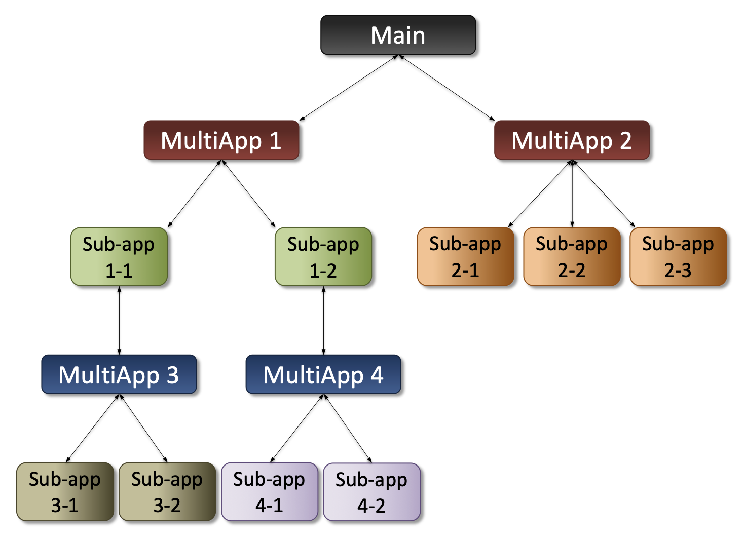
Segregated (loose/tight) coupling achieved using
MultiAppsPhysics coupled via in-memory transfer of fields and scalars
Coupling specified in the input file (no code needed)
No universally superior coupling strategy; correct choice depends on problem
Provides a standardized interface for an analyst to produce a coupled model
MOOSE MultiApp Hierarchy Example
Getting started
Required for upcoming hands-on
Installing a text editor with input file syntax auto-complete
Problem Statement
Consider a system containing two pressure vessels at differing temperatures. The vessels are connected via a pipe that contains a filter consisting of close-packed steel spheres. Predict the velocity and temperature of the fluid inside the filter. The pipe is 0.304 m in length and 0.0514 m in diameter.
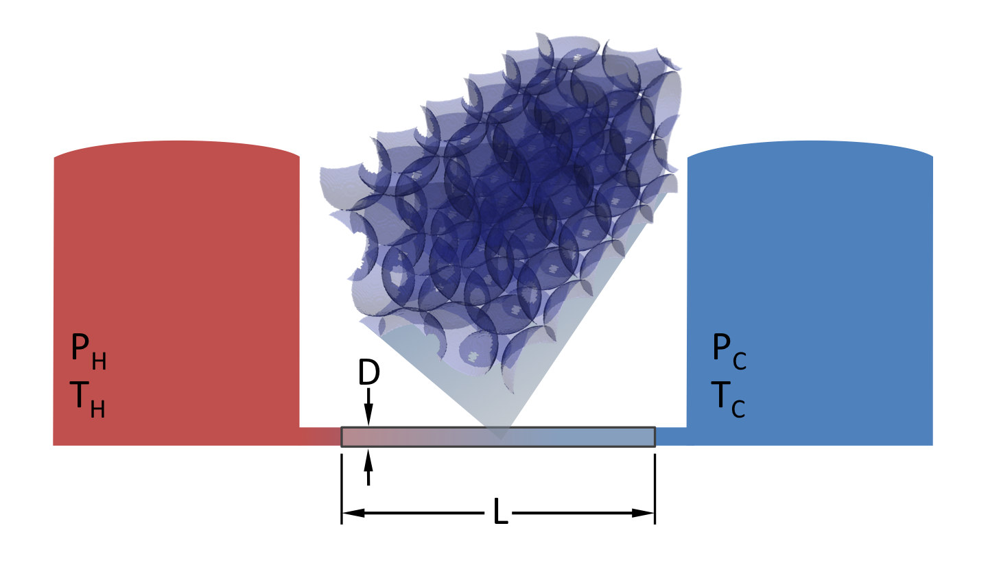
Pamuk and Ozdemir, "Friction factor, permeability, and inertial coefficient of oscillating flow through porous media of packed balls", Experimental Thermal and Fluid Science, v. 38, pp. 134-139, 2012.
Governing Equations
Conservation of Mass:
(1)Conservation of Energy:
(2)Darcy's Law:
(3)where is the fluid velocity, is porosity, is the permeability tensor, is fluid viscosity, is the pressure, is the density, is the specific heat, is the gravity vector, and is the temperature.
Assuming that and imposing the divergence-free condition of Eq. (1) to Eq. (3) leads to the following system of two equations in the unknowns and :
The parameters , , and are the porosity-dependent density, specific heat capacity, and thermal conductivity of the combined fluid/solid medium, defined by:
where is the porosity, is the specific heat, and the subscripts and refer to fluid and solid, respectively.
Material Properties
| Property | Value | Units |
|---|---|---|
| Viscosity of water, | ||
| Density of water, | 995.7 | |
| Density of steel, | 8000 | |
| Thermal conductivity of water, | 0.6 | |
| Thermal conductivity of steel, | 18 | |
| Specific heat capacity of water, | 4181.3 | |
| Specific heat capacity of steel, | 466 |
Tutorial Steps
Step 1: Geometry and Diffusion
The first step is to solve a simple "Diffusion" problem, which requires no code. This step will introduce the basic system of MOOSE.
Step 2: Pressure Kernel
In order to implement the Darcy pressure equation, a Kernel object is needed to represent:
Step 3: Pressure Kernel with Material
Instead of passing constant parameters to the pressure diffusion Kernel object, the Material system can be used to supply the values. This allows for properties that vary in space and time as well as be coupled to variables in the simulation.
Step 4: Velocity Auxiliary Variable
The velocity is computed from the pressure based on Darcy's law as:
This velocity can be computed using the Auxiliary system.
Step 5: Heat Conduction
Solve the transient heat equation using the "heat conduction" module.
Step 6: Equation Coupling
Solve the pressure and temperature in a coupled system of equations by adding the advection term to the heat equation.
Step 7: Mesh Adaptivity
In the transient simulation, a "traveling wave" profile moves through the porous medium. Instead of using a uniform mesh to resolve the wave profile, we can dynamically adapt the mesh to the solution.
Step 8: Postprocessors
Postprocessor and VectorPostprocessor objects can be used to compute aggregate value(s) for a simulation, such as the average temperature on the boundary or the temperatures along a line within the solution domain.
Step 9: Mechanics
Thermal expansion of the porous media can be added to the coupled set of equations using the "solid mechanics" module, without adding additional code.
Step 10: Multiscale Simulation
MOOSE is capable of running multiple applications together and transfer data between the various applications.
This problem replaces the thermal conductivity calculated by the Material with a value computed by another application that runs a phase-based micro-structure simulation.
Step 11: Custom Syntax
MOOSE includes a system to create custom input syntax for common tasks, in this step the syntax for the two equations and velocity auxiliary calculation are simplified for end-users.
Step 1: Geometry and Diffusion
First, consider the steady-state diffusion equation on the domain : find such that
where on the left, on the right and with on the remaining boundaries.
The weak form of this equation, in inner-product notation, is given by:
where are the test functions and is the finite element solution.
Input File(s)
An input file is used to represent the problem in MOOSE. It follows a very standardized syntax.
MOOSE uses the "hierarchical input text" (hit) format.
[Kernels<<<{"href": "../syntax/Kernels/index.html"}>>>]
  [diffusion]
    type = ADDiffusion<<<{"description": "Same as `Diffusion` in terms of physics/residual, but the Jacobian is computed using forward automatic differentiation", "href": "../source/kernels/ADDiffusion.html"}>>> # Laplacian operator using automatic differentiation
    variable<<<{"description": "The name of the variable that this residual object operates on"}>>> = pressure # Operate on the "pressure" variable from above
  []
[]A basic MOOSE input file requires six parts, each of which will be covered in greater detail later.
[Mesh]: Define the geometry of the domain[Variables]: Define the unknown(s) of the problem[Kernels]: Define the equation(s) to solve[BCs]: Define the boundary condition(s) of the problem[Executioner]: Define how the problem will be solved[Outputs]: Define how the solution will be returned
Step 1: Input File
[Mesh<<<{"href": "../syntax/Mesh/index.html"}>>>]
  [gmg]
    type = GeneratedMeshGenerator<<<{"description": "Create a line, square, or cube mesh with uniformly spaced or biased elements.", "href": "../source/meshgenerators/GeneratedMeshGenerator.html"}>>> # Can generate simple lines, rectangles and rectangular prisms
    dim<<<{"description": "The dimension of the mesh to be generated"}>>> = 2                       # Dimension of the mesh
    nx<<<{"description": "Number of elements in the X direction"}>>> = 100                      # Number of elements in the x direction
    ny<<<{"description": "Number of elements in the Y direction"}>>> = 10                       # Number of elements in the y direction
    xmax<<<{"description": "Upper X Coordinate of the generated mesh"}>>> = 0.304                  # Length of test chamber
    ymax<<<{"description": "Upper Y Coordinate of the generated mesh"}>>> = 0.0257                 # Test chamber radius
  []
  coord_type = RZ                 # Axisymmetric RZ
  rz_coord_axis = X               # Which axis the symmetry is around
[]

[Variables<<<{"href": "../syntax/Variables/index.html"}>>>/pressure]
  # Adds a Linear Lagrange variable by default
[]

[Kernels<<<{"href": "../syntax/Kernels/index.html"}>>>/diffusion]
  type = ADDiffusion<<<{"description": "Same as `Diffusion` in terms of physics/residual, but the Jacobian is computed using forward automatic differentiation", "href": "../source/kernels/ADDiffusion.html"}>>>  # Laplacian operator using automatic differentiation
  variable<<<{"description": "The name of the variable that this residual object operates on"}>>> = pressure # Operate on the "pressure" variable from above
[]

[BCs<<<{"href": "../syntax/BCs/index.html"}>>>]
  [inlet]
    type = DirichletBC<<<{"description": "Imposes the essential boundary condition $u=g$, where $g$ is a constant, controllable value.", "href": "../source/bcs/DirichletBC.html"}>>>  # Simple u=value BC
    variable<<<{"description": "The name of the variable that this residual object operates on"}>>> = pressure # Variable to be set
    boundary<<<{"description": "The list of boundary IDs from the mesh where this object applies"}>>> = left     # Name of a sideset in the mesh
    value<<<{"description": "Value of the BC"}>>> = 4000        # (Pa) From Figure 2 from paper.  First data point for 1mm spheres.
  []
  [outlet]
    type = DirichletBC<<<{"description": "Imposes the essential boundary condition $u=g$, where $g$ is a constant, controllable value.", "href": "../source/bcs/DirichletBC.html"}>>>
    variable<<<{"description": "The name of the variable that this residual object operates on"}>>> = pressure
    boundary<<<{"description": "The list of boundary IDs from the mesh where this object applies"}>>> = right
    value<<<{"description": "Value of the BC"}>>> = 0           # (Pa) Gives the correct pressure drop from Figure 2 for 1mm spheres
  []
[]

[Problem<<<{"href": "../syntax/Problem/index.html"}>>>]
  type = FEProblem  # This is the "normal" type of Finite Element Problem in MOOSE
[]

[Executioner<<<{"href": "../syntax/Executioner/index.html"}>>>]
  type = Steady       # Steady state problem
  solve_type = NEWTON # Perform a Newton solve, uses AD to compute Jacobian terms
  petsc_options_iname = '-pc_type -pc_hypre_type' # PETSc option pairs with values below
  petsc_options_value = 'hypre boomeramg'
[]

[Outputs<<<{"href": "../syntax/Outputs/index.html"}>>>]
  exodus<<<{"description": "Output the results using the default settings for Exodus output."}>>> = true # Output Exodus format
[]Step 1: Run
An executable is produced by compiling an application or a MOOSE module. It can be used to run input files.
cd ~/projects/moose/tutorials/darcy_thermo_mech/step01_diffusion
make -j 12 # use number of processors for your system
cd problems
../darcy_thermo_mech-opt -i step1.i
Step 1: Result

Finite Element Method (FEM)
Function Approximation
To introduce the concept of FEM, consider a polynomial regression exercise. We can search for a polynomial function that solves the following problems:
Discrete example: Given sampled locations with associated values, we want our polynomial function to be as close to the input data as possible.
Continuous example: Given a complicated function, we want to have our polynomial function as close to the input function as possible.
Let us write the polynomial in the following form:
where are scalar coefficients (expansion coefficients) and monomials are "basis functions". Thus, the problem is to find such that is closest the the given points or a given function.
Polynomial Example (Discrete)
Define a set of points (Let's pick the points using ):
Substitute data into the polynomial model:
This results 4 equations for 3 unknowns () that can be expressed as the following linear system:
We want to get the function closest to the points. Distance in this case can be expressed by the discrete norm:
We want to minimize the norm of the squared distances ("least squares"):
which requires the solution of this problem:
which results in:
These coefficients define the solution function:
Polynomial Example (Continuous)
We want to minimize the squared distance between the known function () and the polynomial approximate () on a given domain :
The cumulative squared distance can be expressed as:
which we would like to minimize in a least-squares sense, with respect to the coefficients in (entries of ):
We can move the derivative with respect to into the integral:
which results in the following system (dropping the factor 2):
with
solving this sytem results in:
These coefficients define the solution function:
The coefficients are meaningless, they are just numbers used to define a function.
The solution is not the coefficients, but rather the function created when they are multiplied by their respective basis functions and summed.
The function is defined everywhere in the domain.
can be evaluated at the point , for example, by computing:
where the correspond to the coefficients in the solution vector, and the are the respective functions.
FEM can be used to solve both linear and nonlinear PDEs
FEM is a method for numerically approximating the solution to partial differential equations (PDEs). FEM is widely applicable for a large range of PDEs and domains.
Example PDEs: Have you seen them before? Are they linear/nonlinear? Coupled?
(4)(5)(6)FEM is a general method to discretize these equations
FEM finds a solution function that is made up of "shape functions" multiplied by coefficients and added together, just like in polynomial regression, except the functions are not typically as simple (although they can be).
The Galerkin Finite Element method is different from finite difference and finite volume methods because it finds a piecewise continuous function which is an approximate solution to the governing PDEs.
FEM provides an approximate solution. The true solution can only be represented as well as the shape function basis can represent it!
FEM is supported by a rich mathematical theory with proofs about accuracy, stability, convergence and solution uniqueness.
Weak Form
Using FEM to find the solution to a PDE starts with forming a "weighted residual" or "variational statement" or "weak form", this processes if referred to here as generating a weak form.
The weak form provides flexibility, both mathematically and numerically and it is needed by MOOSE to solve a problem.
Generating a weak form generally involves these steps:
Write down strong form of PDE.
Rearrange terms so that zero is on the right of the equals sign.
Multiply the whole equation by a "test" function .
Integrate the whole equation over the domain .
Integrate by parts and use the divergence theorem to get the desired derivative order on your functions and simultaneously generate boundary integrals.
Obtain the weak form for the equations listed on the previous slide and the shape functions.
Looking back
Polynomial fitting:
Form equations that the coefficients of a polynomial function must satisfy to fit
Solve the linear system
Reconstruct the fit by evaluating the polynomial defined by its coefficients
Finite Element method:
Form equations on each element to minimize the residual of an equation
Solve the linear system
Reconstruct the function
Re-evaluate the equation and iterate (for nonlinear equations)
Integration by Parts and Divergence Theorem
Suppose is a scalar function, is a vector function, and both are continuously differentiable functions, then the product rule states:
The function can be integrated over the volume and rearranged as:
(7)The divergence theorem transforms a volume integral into a surface integral on surface :
(8)where is the outward normal vector for surface . Combining Eq. (7) and Eq. (8) yield:
(9)Example: Advection-Diffusion
(1) Write the strong form of the equation:
(2) Rearrange to get zero on the right-hand side:
(3) Multiply by the test function :
(4) Integrate over the domain :
(5) Integrate by parts and apply the divergence theorem, by using Eq. (9) on the left-most term of the PDE:
Write in inner product notation. Each term of the equation will inherit from an existing MOOSE type as shown below.
(10)Corresponding MOOSE input file blocks
[Kernels<<<{"href": "../syntax/Kernels/index.html"}>>>]
  [diffusion]
    type = CoefDiffusion<<<{"description": "Kernel for diffusion with diffusivity = coef + function", "href": "../source/kernels/CoefDiffusion.html"}>>>
    variable<<<{"description": "The name of the variable that this residual object operates on"}>>> = 'u'
    coef<<<{"description": "Diffusion coefficient"}>>> = ${k}
  []
[]
[BCs<<<{"href": "../syntax/BCs/index.html"}>>>]
[inlet_flux]
type = FunctionNeumannBC<<<{"description": "Imposes the integrated boundary condition $\\frac{\\partial u}{\\partial n}=h(t,\\vec{x})$, where $h$ is a (possibly) time and space-dependent MOOSE Function.", "href": "../source/bcs/FunctionNeumannBC.html"}>>>
variable<<<{"description": "The name of the variable that this residual object operates on"}>>> = 'u'
boundary<<<{"description": "The list of boundary IDs from the mesh where this object applies"}>>> = 'left'
function<<<{"description": "The function."}>>> = box_flux
[]
[outlet_avective_flux]
type = ConservativeAdvectionBC<<<{"description": "Boundary condition for advection when it is integrated by parts. Supports Dirichlet (inlet-like) and implicit (outlet-like) conditions.", "href": "../source/bcs/ConservativeAdvectionBC.html"}>>>
variable<<<{"description": "The name of the variable that this residual object operates on"}>>> = 'u'
boundary<<<{"description": "The list of boundary IDs from the mesh where this object applies"}>>> = 'right'
velocity_function<<<{"description": "Function describing the values of velocity on the boundary."}>>> = 'beta'
[]
[outlet_diffusive_flux]
type = DiffusionFluxBC<<<{"description": "Computes a boundary residual contribution consistent with the Diffusion Kernel. Does not impose a boundary condition; instead computes the boundary contribution corresponding to the current value of grad(u) and accumulates it in the residual vector.", "href": "../source/bcs/DiffusionFluxBC.html"}>>>
variable<<<{"description": "The name of the variable that this residual object operates on"}>>> = 'u'
boundary<<<{"description": "The list of boundary IDs from the mesh where this object applies"}>>> = 'right'
[]
# walls are 0 flux (achieved with no BC, this depends on the kernels used)
[][Kernels<<<{"href": "../syntax/Kernels/index.html"}>>>]
[advection]
type = ConservativeAdvection<<<{"description": "Conservative form of $\\nabla \\cdot \\vec{v} u$ which in its weak form is given by: $(-\\nabla \\psi_i, \\vec{v} u)$. Velocity can be given as 1) a variable, for which the gradient is automatically taken, 2) a vector variable, or a 3) vector material.", "href": "../source/kernels/ConservativeAdvection.html"}>>>
variable<<<{"description": "The name of the variable that this residual object operates on"}>>> = u
velocity = ${beta}
[]
[][Kernels<<<{"href": "../syntax/Kernels/index.html"}>>>]
[force]
type = BodyForce<<<{"description": "Demonstrates the multiple ways that scalar values can be introduced into kernels, e.g. (controllable) constants, functions, and postprocessors. Implements the weak form $(\\psi_i, -f)$.", "href": "../source/kernels/BodyForce.html"}>>>
variable<<<{"description": "The name of the variable that this residual object operates on"}>>> = u
function<<<{"description": "A function that describes the body force"}>>> = f_fn
[]
[]Finite Element Shape Functions
Basis Functions
While the weak form is essentially what is needed for adding physics to MOOSE, in traditional finite element software more work is necessary.
The weak form must be discretized using a set of "basis functions" amenable for manipulation by a computer.

Images copyright Becker et al. (1981)

Shape Functions
The discretized expansion of takes on the following form:
where are the "basis functions", which form the basis for the "trial function", . is the total number of functions for the discretized domain.
The gradient of can be expanded similarly:
In the Galerkin finite element method, the same basis functions are used for both the trial and test functions:
Substituting these expansions back into the example weak form (Eq. (10)) yields:
(11)The left-hand side of the equation above is referred to as the component of the "residual vector," .
Shape Functions are the functions that get multiplied by coefficients and summed to form the solution.
Individual shape functions are restrictions of the global basis functions to individual elements.
They are analogous to the functions from polynomial fitting (in fact, you can use those as shape functions).
Typical shape function families: Lagrange, Hermite, Hierarchic, Monomial, Clough-Tocher
Lagrange shape functions are the most common, which are interpolatory at the nodes, i.e., the coefficients correspond to the values of the functions at the nodes.
Example 1D Shape Functions


2D Lagrange Shape Functions
Example bi-quadratic basis functions defined on the (square) Quad9 element:
(left) is associated to a "corner" node, it is zero on the opposite edges.
(middle) is associated to a "mid-edge" node, it is zero on all other edges.
(right) is associated to the "center" node, it is symmetric and on the element.


Setting Shape Functions in a MOOSE input file
Shape functions can be set for each variable in the Variables block:
[Variables<<<{"href": "../syntax/Variables/index.html"}>>>]
  [u]
    order<<<{"description": "Specifies the order of the FE shape function to use for this variable (additional orders not listed are allowed)"}>>> = FIRST
    family<<<{"description": "Specifies the family of FE shape functions to use for this variable"}>>> = LAGRANGE
    block = 0
  []
  [v]
    order<<<{"description": "Specifies the order of the FE shape function to use for this variable (additional orders not listed are allowed)"}>>> = FIRST
    family<<<{"description": "Specifies the family of FE shape functions to use for this variable"}>>> = LAGRANGE
    block = 1
  []
[]Numerical Implementation
Numerical Integration
The only remaining non-discretized parts of the weak form are the integrals. First, split the domain integral into a sum of integrals over elements:
(12)Through a change of variables, the element integrals are mapped to integrals over the "reference" elements .
where is the Jacobian of the map from the physical element to the reference element.
Reference Element (Quad9)

Quadrature
Quadrature, typically "Gaussian quadrature", is used to approximate the reference element integrals numerically.
where is the weight function at quadrature point .
Under certain common situations, the quadrature approximation is exact. For example, in 1 dimension, Gaussian Quadrature can exactly integrate polynomials of order with quadrature points.
Applying the quadrature to Eq. (12) we can simply compute:
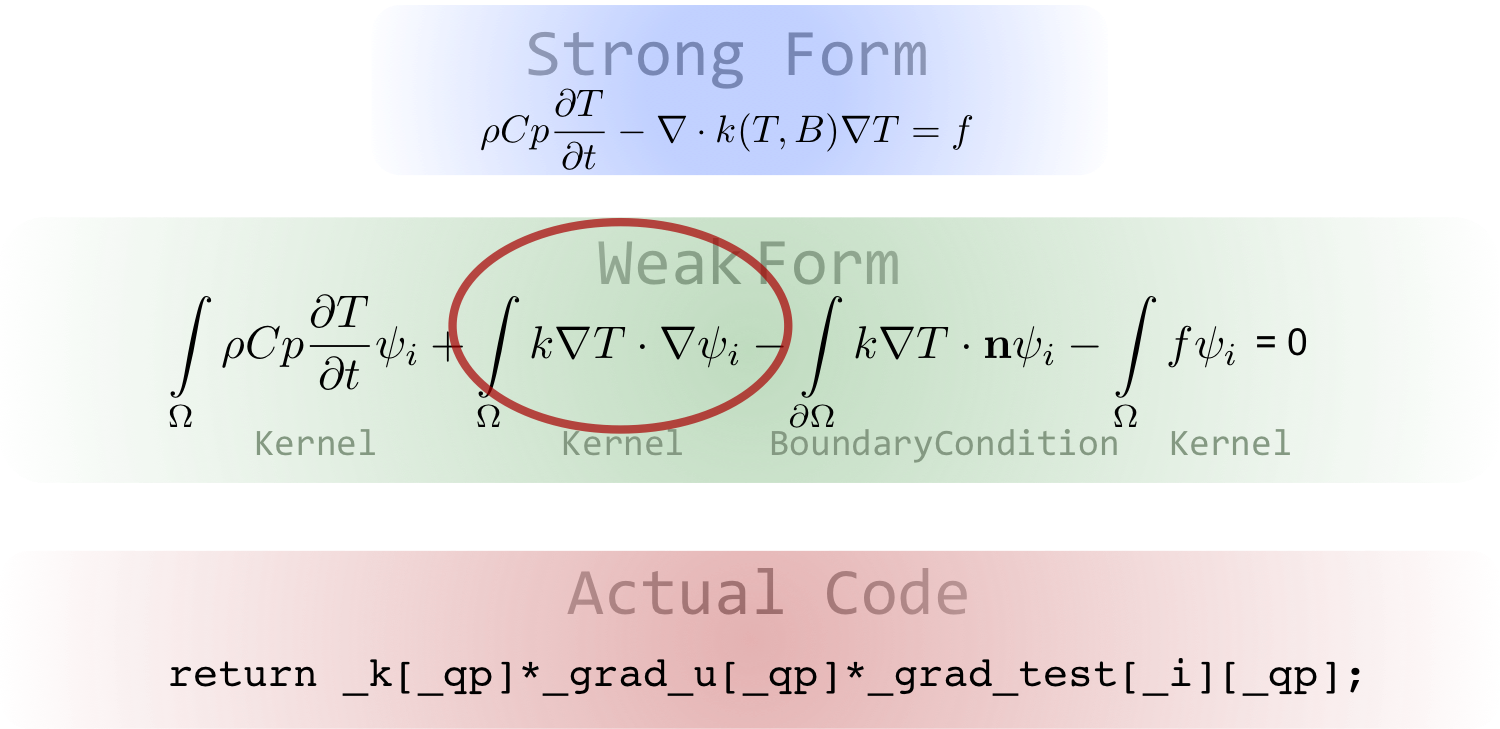
where is the spatial location of the quadrature point and is its associated weight.
MOOSE handles multiplication by the Jacobian () and the weight () automatically, thus your Kernel object is only responsible for computing the part of the integrand.
Sampling at the quadrature points yields:
Thus, the weak form of Eq. (11) becomes:
(13)The second sum is over boundary faces, . MOOSE Kernel or BoundaryCondition objects provide each of the terms in square brackets (evaluated at or as necessary), respectively.
Intermediate summary
There is a mesh, with cells and functions, polynomials, defined by their coefficients
We plug in these functions in the PDEs, then obtain a weak form
We evaluate the integrals in the weak form using a quadrature, thus forming a set of equations
Now let's solve these equations to obtain the coefficients
Newton's Method
Newton's method is a "root finding" method with good convergence properties, in "update form", for finding roots of a scalar equation it is defined as: , is given by

Newton's Method in MOOSE
The residual, , as defined by Eq. (13) is a nonlinear system of equations,
that is used to solve for the coefficients .
For this system of nonlinear equations Newton's method is defined as:
(14)where is the Jacobian matrix evaluated at the current iterate:
MOOSE Solve Types
The solve type is specified in the [Executioner] block within the input file:
[Executioner]
  solve_type = PJFNK
Available options include:
PJFNK: Preconditioned Jacobian Free Newton Krylov (default)
JFNK: Jacobian Free Newton Krylov
NEWTON: Performs solve using exact Jacobian for preconditioning
FD: PETSc computes terms using a finite difference method (debug)
JFNK
Uses a Krylov subspace-based linear solver
(15)The action of the Jacobian is approximated by:
(16)The Kernel method computeQpResidual is called to compute during the nonlinear step (Eq. (14)).
During each linear step of JFNK, the computeQpResidual method is called to approximate the action of the Jacobian on the Krylov vector.
PJFNK
The action of the preconditioned Jacobian is approximated by:
(17)The Kernel method computeQpResidual is called to compute during the nonlinear step (Eq. (14)).
During each linear step of PJFNK, the computeQpResidual method is called to approximate the action of the Jacobian on the Krylov vector. The computeQpJacobian and computeQpOffDiagJacobian methods are used to compute values for the preconditioning matrix.
NEWTON
The Kernel method computeQpResidual is called to compute during the nonlinear step (Eq. (14)).
The computeQpJacobian and computeQpOffDiagJacobian methods are used to compute the preconditioning matrix. It is assumed that the preconditioning matrix is the Jacobian matrix, thus the residual and Jacobian calculations are able to remain constant during linear iterations.
Preconditioning
Select a preconditioner using PETSC options, either in the executioner or in the [Preconditioning] block:
[Executioner]
  type = Steady
  petsc_options_iname = '-pc_type -pc_hypre_type'
  petsc_options_value = 'hypre boomeramg'
Some examples:
LU : form the actual Jacobian inverse, useful for small to medium problems but does not scale well
Hypre BoomerAMG : algebraic multi-grid, works well for diffusive problems
Jacobi : preconditions with the diagonal, row sum, or row max of Jacobian
For parallel preconditioners, the sub-block (on-process) preconditioners can be controlled with the PETSc option -sub_pc_type. E.g. for a parallel block Jacobi preconditioner (-pc_type bjacobi) the sub-block preconditioner could be set to ILU or LU etc. with -sub_pc_type ilu, -sub_pc_type lu, etc.
Summary
The Finite Element Method is a way of numerically approximating the solution of PDEs.
Just like polynomial fitting, FEM finds coefficients for basis functions.
The solution is the combination of the coefficients and the basis functions, and the solution can be sampled anywhere in the domain.
Integrals are computed numerically using quadrature.
Newton's method provides a mechanism for solving a system of nonlinear equations.
The Preconditioned Jacobian Free Newton Krylov (PJFNK) method allows us to avoid explicitly forming the Jacobian matrix while still computing its action.
Automatic Jacobian Calculation
MOOSE uses forward mode automatic differentiation from the MetaPhysicL package.
Moving forward, the idea is for application developers to be able to develop entire apps without writing a single Jacobian statement. This has the potential to decrease application development time.
In terms of computing performance, presently AD Jacobians are slower to compute than hand-coded Jacobians, but they parallelize extremely well and can benefit from using a NEWTON solve, which often results in decreased solve time overall.
Relies on two techniques:
chain rule
operator overloading
One thing to note is that the derivatives are with regards to the degrees of freedom, but the residual is computed at quadrature points! There are therefore often several non-zero coefficients even for simply (value of variable u at a quadrature point).
Manual Jacobian Calculation
The remainder of the tutorial will focus on using automatic differentiation (AD) for computing Jacobian terms, but it is possible to compute them manually.
It is recommended that all new Kernel objects use AD.
FEM Derivative Identities
The following relationships are useful when computing Jacobian terms.
(18)(19)Newton for a Simple Equation
Again, consider the advection-diffusion equation with nonlinear , , and :
Thus, the component of the residual vector is:
Using the previously-defined rules in Eq. (18) and Eq. (19) for and , the entry of the Jacobian is then:
That even for this "simple" equation, the Jacobian entries are nontrivial: they depend on the partial derivatives of , , and , which may be difficult or time-consuming to compute analytically.
In a multiphysics setting with many coupled equations and complicated material properties, the Jacobian might be extremely difficult to determine.
C++
Fundamentals
Data Types
| Intrinsic Type | Variant(s) |
|---|---|
| bool | | |
| char | unsigned |
| int | unsigned, long, short |
| float | | |
| double | long |
| void | | |
Note, void is the "anti-datatype", used in functions returning nothing
Objects of these types can be combined into more complicated "structure" or "class" objects, or aggregated into arrays or various "container" classes.
Operators
| Purpose | Symbols |
|---|---|
| Math | + - * / % += -= /= %= ++ -- |
| Comparison | < > <= >= != == |
| Logical Comparison | && || ! |
| Memory | * & new delete sizeof |
| Assignment | = |
| Member Access | -> . |
| Name Resolution | :: |
Curly Braces { }
Used to group statements together and to define the scope of a function
Creates new layer of scope
int x = 2;

{
  int x = 5; // "Shadows" the other x - bad practice
  assert(x == 5);
}

assert(x == 2);
Expressions
Composite mathematical expressions:
a = b * (c - 4) / d++;
Composite boolean expressions:
if (a && b && f()) { e = a; }
Note, Operators && and || use "short-circuiting," so "b" and "f()" in the example above may not get evaluated.
Scope resolution:
a = std::pow(r, 2);     // Calls the standard pow() function
b = YourLib::pow(r, 2); // Calls pow() from YourLib namespace or class

using std::pow;      // Now "pow" can mean "std::pow" automatically
using YourLib::pow;  // Or it can mean "YourLib::pow"...

c = pow(r, 2); // Ambiguous, or deduced from the type of r
Dot and Pointer Operator:
t = my_obj.someFunction();
b = my_ptr->someFunction();
Type Casting
float pi = 3.14;
int approx_pi = static_cast<int>(pi);
Limits to Type Casting
Does not work to change to fundamentally different types
float f = (float) "3.14"; // won't compile
Be careful with your assumptions
unsigned int huge_value = 4294967295; // ok
int i = huge_value;                   // value silently changed!
int j = static_cast<int>(huge_value); // won't help!
And consider safer MOOSE tools
int i = cast_int<int>(huge_value); // assertion failure in non-optimized runs
Control Statements
For, While, and Do-While Loops:
for (int i=0; i<10; ++i) { foo(i); }
for (auto val : my_container) { foo(val); }
while (boolean-expression)  { bar(); }
do { baz(); } while (boolean-expression);
If-Then-Else Tests:
if (boolean-expression) { }
else if (boolean-expression) { }
else { }
In the previous examples, boolean-expression is any valid C++ statement which results in true or false, such as:
if (0) // Always falsewhile (a > 5)
Declarations and Definitions
In C++ we split our code into multiple files
headers (*.h)
bodies (*.C)
Headers generally contain declarations
Statement of the types we will use
Gives names to types
The argument and return type signatures of functions
Bodies generally contain definitions
Our descriptions of those types, including what they do or how they are built
Memory consumed
The operations functions perform
Declaration Examples
Free functions:
returnType functionName(type1 name1, type2 name2);
Object member functions (methods):
class ClassName
{
  returnType methodName(type1 name1, type2 name2);
};
(Pointers to) functions themselves are also objects, with ugly syntax
  returnType (*f_ptr)(type1, type2) = &functionName;
  returnType r = (*f_ptr)(a1, a2);
  do_something_else_with(f_ptr);
Definition Examples
Function definition:
returnType functionName(type1 name1, type2 name2)
{
  // statements
}
Class method definition:
returnType ClassName::methodName(type1 name1, type2 name2)
{
   // statements
}
Make
A Makefile is a list of dependencies with rules to satisfy those dependencies. All MOOSE-based applications are supplied with a complete Makefile.
To build a MOOSE-based application, just type:
make
C++
Scope, Memory, and Overloading
Scope
A scope is the extent of the program where a variable can be seen and used.
local variables have scope from the point of declaration to the end of the enclosing block { }
global variables are not enclosed within any scope and are available within the entire file
Variables have a limited lifetime
When a variable goes out of scope, its destructor is called
Manually dynamically-allocated (via new) memory is not automatically freed at the end of scope, but smart-pointers and containers will free dynamically-allocated memory in their destructors.
Scope Resolution Operator
"double colon" :: is used to refer to members inside of a named scope
// definition of the "myMethod" function of "MyObject"
void MyObject::myMethod()
{
  std::cout << "Hello, World!\n";
}
MyNamespace::a = 2.718;
MyObject::myMethod();
Namespaces permit data organization, but do not have all the features needed for full encapsulation
Assignment
(Prequel to Pointers and Refs)
Recall that assignment in C++ uses the "single equals" operator:
a = b; // Assignment
Assignments are one of the most common operations in programming
Two operands are required
An assignable "lvalue" on the left hand side, referring to some object
An expression on the right hand side
Pointers
Native type just like an int or long
Hold the location of another variable or object in memory
Useful in avoiding expensive copies of large objects
Facilitate shared memory
Example: One object "owns" the memory associated with some data, and allows others objects access through a pointer
Pointer Syntax
Declare a pointer
int *p;
The address-of operator on a variable gives a pointer to it, for initializing another pointer
int a;
p = &a;
The dereference operator on a pointer gives a reference to what it points to, to get or set values
*p = 5;                  // set value of "a" through "p"
std::cout << *p << "\n"; // prints 5
std::cout <<  a << "\n"; // prints 5
Pointer Syntax (continued)
int a = 5;
int *p;       // declare a pointer
p = &a;       // set 'p' equal to address of 'a'
*p = *p + 2;  // get value pointed to by 'p', add 2,
              // store result in same location
std::cout <<  a << "\n";  // prints 7
std::cout << *p << "\n";  // prints 7
std::cout <<  p << "\n";  // prints an address (0x7fff5fbfe95c)
Pointers are Powerful but Unsafe
On the previous slide we had this:
p = &a;
But we can do almost anything we want with p!
p = p + 1000;
Now what happens when we do this?
*p; // Access memory at &a + 1000
References to the Rescue
A reference is an alternative name for an object (Stroustrup), like an alias for the original variable
int a = 5;
int &r = a;  // define and initialize a ref
r = r + 2;
std::cout <<  a << "\n";  // prints 7
std::cout <<  r << "\n";  // prints 7
std::cout << &r << "\n";  // prints address of a
References are Safer
References cannot be reseated, nor left un-initialized - even classes with references must initialize them in the constructor!
&r = &r + 1;   // won't compile
int &r;        // won't compile
But references can still be incorrectly left "dangling"
std::vector<int> four_ints(4);
int &r = four_ints[0];
r = 5;  // Valid: four_ints is now {5,0,0,0}
four_ints.clear();  // four_ints is now {}
r = 6;  // Undefined behavior, nasal demons
Rvalue References Can Be More Efficient
An "lvalue" reference starts with &; an "rvalue" reference starts with &&.
Mnemonic: lvalues can usually be assigned to, Left of an = sign; rvalues can't, so they're found Right of an = sign.
Lvalue code like "copy assignment" is correct and sufficient
Foo & Foo::operator= (const Foo & other) {
  this->member1 = other.member1;  // Has to copy everything
  this->member2 = other.member2;
}
But rvalue code like "move assignment" may be written for optimization
Foo & Foo::operator= (Foo && other) {
  // std::move "makes an lvalue into an rvalue"
  this->member1 = std::move(other.member1);  // Can cheaply "steal" memory
  this->member2 = std::move(other.member2);
}
Summary: Pointers and References
A pointer is a variable that holds a potentially-changeable memory address to another variable
int *iPtr;  // Declaration
iPtr = &c;
int a = b + *iPtr;
An lvalue reference is an alternative name for an object, and must reference a fixed object
int &iRef = c;    // Must initialize
int a = b + iRef;
An rvalue reference is an alternative name for a temporary object
std::sqrt(a + b); // "a+b" creates an object which will stop existing shortly
Calling Conventions
What happens when you make a function call?
result = someFunction(a, b, my_shape);
If the function changes the values inside of a, b or myshape, are those changes reflected in my code?
Is this call expensive? (Are arguments copied around?)
C++ by default is "Pass by Value" (copy) but you can pass arguments by reference (alias) with additional syntax
"Swap" Example - Pass by Value
void swap(int a, int b)
{
  int temp = a;
  a = b;
  b = temp;
}
int i = 1;
int j = 2;
swap (i, j);                  // i and j are arguments
std::cout << i << " " << j;   // prints 1 2
                              // i and j are not swapped
Swap Example - Pass by (Lvalue) Reference
void swap(int &a, int &b)
{
  int temp = a;
  a = b;
  b = temp;
}
int i = 1;
int j = 2;
swap (i, j);                  // i and j are arguments
std::cout << i << " " << j;   // prints 2 1
                              // i and j are properly swapped
Dynamic Memory Allocation
Why do we need dynamic memory allocation?
Data size specified at run time (rather than compile time)
Persistence without global variables (scopes)
Efficient use of space
Flexibility
Dynamic Memory in C++
"new" allocates memory, "delete" frees it
Recall that variables typically have limited lifetimes (within the nearest enclosing scope)
Dynamic memory allocations do not have limited lifetimes
No deallocation when a pointer goes out of scope!
No automatic garbage collection when dynamic memory becomes unreachable!
Watch out for memory leaks - a missing "delete" is memory that is lost until program exit
Modern C++ provides classes that encapsulate allocation, with destructors that deallocate.
Almost every "new"/"delete" should be a "smart pointer" or container class instead!
Example: Dynamic Memory
  {
    int a = 4;
    int *b = new int; // dynamic allocation; what is b's value?
    auto c = std::make_unique<int>(6); // dynamic allocation
    *b = 5;
    int d = a + *b + *c;
    std::cout << d;  // prints 15
  }
  // a, b, and c are no longer on the stack
  // *c was deleted from the heap by std::unique_ptr
  // *b is leaked memory - we forgot "delete b" and now it's too late!
Example: Dynamic Memory Using References
int a;
auto b = std::make_unique<int>(); // dynamic allocation
int &r = *b;     // creating a reference to newly allocated object
a = 4;
r = 5;
int c = a + r;
std::cout << c;  // prints 9
Const
The const keyword is used to mark a variable, parameter, method or other argument as constant
Often used with references and pointers to share objects which should not be modified
{
  std::string name("myObject");
  print(name);
}
void print(const std::string & name)
{
  name = "MineNow"; // Compile-time error
  const_cast<std::string &>(name) = "MineNow"; // Just bad code
  ...
}
Constexpr
The constexpr keyword marks a variable or function as evaluable at compile time
constexpr int factorial(int n)
{
  if (n <= 1)
    return 1;
  return n * factorial(n-1);
}
{
  constexpr int a = factorial(6); // Compiles straight to a = 720
  int b = 6;
  function_which_might_modify(b);
  int c = factorial(b); // Computed at run time
}
Function Overloading
In C++ you may reuse function names as long as they have different parameter lists or types. A difference only in the return type is not enough to differentiate overloaded signatures.
int foo(int value);
int foo(float value);
int foo(float value, bool is_initialized);
...
This is very useful when we get to object "constructors".
C++
Types, Templates, and
Standard Template Library (STL)
Static vs Dynamic Type Systems
C++ is a "statically-typed" language
This means that "type checking" is performed at compile time as opposed to at run time
Python and MATLAB are examples of "dynamically-typed" languages
Static Typing Pros and Cons
Pros:
Safety: compilers can detect many errors
Optimization: compilers can optimize for size and speed
Documentation: flow of types and their uses in expression is self documenting
Cons:
More explicit code is needed to convert ("cast") between types
Abstracting or creating generic algorithms is more difficult
Templates
C++ implements the generic programming paradigm with "templates".
Many of the finer details of C++ template usage are beyond the scope of this short tutorial.
Fortunately, only a small amount of syntactic knowledge is required to make effective basic use of templates.
template <class T>
T getMax (T a, T b)
{
  if (a > b)
    return a;
  else
    return b;
}
Templates (continued)
template <class T>
T getMax (T a, T b)
{
  return (a > b ? a : b); // "ternary" operator
}
int i = 5, j = 6, k;
float x = 3.142; y = 2.718, z;
k = getMax(i, j);       // uses int version
z = getMax(x, y);       // uses float version
k = getMax<int>(i, j);  // explicitly calls int version
Template Specialization
template<class T>
void print(T value)
{
  std::cout << value << std::endl;
}

template<>
void print<bool>(bool value)
{
  if (value)
    std::cout << "true\n";
  else
    std::cout << "false\n";
}
Template Specialization (continued)
int main()
{
  int a = 5;
  bool b = true;
  print(a); // prints 5
  print(b); // prints true
}
C++ Standard Template Library Classes
C++
Classes and Object Oriented Programming
Object Oriented Definitions
A "class" is a new data type that contains data and methods for operating on that data
Think of it as a "blue print" for building an object
An "interface" is defined as a class's publicly available "methods" and "members"
An "instance" is a variable of one of these new data types.
Also known as an "object"
Analogy: You can use one "blue-print" to build many buildings. You can use one "class" to build many "objects".
Object Oriented Design
Instead of manipulating data, one manipulates objects that have defined interfaces
Data encapsulation is the idea that objects or new types should be black boxes. Implementation details are unimportant as long as an object works as advertised without side effects.
Inheritance gives us the ability to abstract or "factor out" common data and functions out of related types into a single location for consistency (avoids code duplication) and enables code re-use.
Polymorphism gives us the ability to write generic algorithms that automatically work with derived types.
Encapsulation (Point.h)
class Point
{
public:
  Point(float x, float y);   // Constructor

  // Accessors
  float getX();
  float getY();
  void setX(float x);
  void setY(float y);
private:
  float _x, _y;
};
Constructors
The method that is called explicitly or implicitly to build an object
Always has the same name as the class with no return type
May have many overloaded versions with different parameters
The constructor body uses a special syntax for initialization called an initialization list
Every member that can be initialized in the initialized list - should be
References have to be initialized here
Point Class Definitions (Point.C)
#include "Point.h"

Point::Point(float x, float y): _x(x), _y(y) { }
float Point::getX() { return _x; }
float Point::getY() { return _y; }
void Point::setX(float x) { _x = x; }
void Point::setY(float y) { _y = y; }
The data is safely encapsulated so we can change the implementation without affecting users of this type
Changing the Implementation (Point.h)
class Point
{
public:
  Point(float x, float y);
  float getX();
  float getY();
  void setX(float x);
  void setY(float y);
private:
  // Store a vector of values rather than separate scalars
  std::vector<float> _coords;
};
New Point Class Body (Point.C)
#include "Point.h"
Point::Point(float x, float y)
{
  _coords.push_back(x);
  _coords.push_back(y);
}

float Point::getX() { return _coords[0]; }
float Point::getY() { return _coords[1]; }
void Point::setX(float x) { _coords[0] = x; }
void Point::setY(float y) { _coords[1] = y; }
Using the Point Class (main.C)
#include "Point.h"
int main()
{
  Point p1(1, 2);
  Point p2 = Point(3, 4);
  Point p3; // compile error, no default constructor
  std::cout << p1.getX() << "," << p1.getY() << "\n"
            << p2.getX() << "," << p2.getY() << "\n";
}
Operator Overloading
For some user-defined types (objects) it makes sense to use built-in operators to perform functions with those types
For example, without operator overloading, adding the coordinates of two points and assigning the result to a third object might be performed like this:
Point a(1,2), b(3,4), c(5,6);
// Assign c = a + b using accessors
c.setX(a.getX() + b.getX());
c.setY(a.getY() + b.getY());
However the ability to reuse existing operators on new types makes the following possible:
c = a + b;
Operator Overloading (continued)
Inside our Point class, we define new member functions with the special operator keyword:
Point Point::operator+(const Point & p)
{
  return Point(_x + p._x, _y + p._y);
}

Point & Point::operator=(const Point & p)
{
  _x = p._x;
  _y = p._y;
  return *this;
}
Using "Point" with Operators
#include "Point.h"

int main()
{
  Point p1(0, 0), p2(1, 2), p3(3, 4);
  p1 = p2 + p3;
  std::cout << p1.getX() << "," << p1.getY() << "\n";
}
A More Advanced Example (Shape.h)
class Shape {
public:
  Shape(int x=0, int y=0): _x(x), _y(y) {}  // Constructor
  virtual ~Shape() {} // Destructor
  virtual float area() const = 0;  // Pure Virtual Function
  void printPosition() const;    // Body appears elsewhere

protected:
  // Coordinates at the centroid of the shape
  int _x;
  int _y;
};
The Derived Class: Rectangle.h
#include "Shape.h"
class Rectangle: public Shape
{
public:
  Rectangle(int width, int height, int x=0, int y=0) :
    Shape(x,y),
    _width(width),
    _height(height)
  {}

  virtual float area() const override { return _width * _height; }

protected:
  int _width;
  int _height;
};
A Derived Class: Circle.h
#include "Shape.h"
class Circle: public Shape
{
public:
  Circle(int radius, int x=0, int y=0) :
    Shape(x,y),
    _radius(radius)
  {}

  virtual float area() const override { return PI * _radius * _radius; }
protected:
  int _radius;
  const double PI = 3.14159265359;
};
Inheritance (Is a...)
When using inheritance, the derived class can be described in terms of the base class
A Rectangle "is a" Shape
Derived classes are "type" compatible with the base class (or any of its ancestors)
We can use a base class variable to point to or refer to an instance of a derived class
Rectangle rectangle(3, 4);
Shape & s_ref = rectangle;
Shape * s_ptr = &rectangle;
Deciphering Long Declarations
Read the declaration from right to left
// mesh is a pointer to a Mesh object
Mesh * mesh;

// params is a reference to an InputParameters object
InputParameters & params;

// the following are identical
// value is a reference to a constant Real object
const Real & value;
Real const & value;
Writing a Generic Algorithm
// create a couple of shapes
Rectangle r(3, 4);
Circle c(3, 10, 10);
printInformation(r);   // pass a Rectangle into a Shape reference
printInformation(c);   // pass a Circle into a Shape reference
...
void printInformation(const Shape & shape)
{
  shape.printPosition();
  std::cout << shape.area() << '\n';
}
// (0, 0)
// 12
// (10, 10)
// 28.274
Summary
Templates
compile-time polymorphism
slower to compile
must be instantiated to be compiled
Classes
run-time polymorphism: routine calls forwarded to derived classes
slower execution due to cost of virtual table lookups
easier to develop with, somewhat more readable
Both enable better code re-use, lower duplication. They have different tradeoffs, but both concepts can be combined! For example:
// class template
template<typename T> class A { };
Homework Ideas
Implement a new Shape called Square. Try deriving from Rectangle directly instead of Shape. What advantages/disadvantages do the two designs have?
Implement a Triangle shape. What interesting subclasses of Triangle can you imagine?
Add another constructor to the Rectangle class that accepts coordinates instead of height and width.
MOOSE C++ Standard
Clang Format
MOOSE uses "clang-format" to automatically format code:
git clang-format branch_name_here
Single spacing around all binary operators
No spacing around unary operators
No spacing on the inside of brackets or parenthesis in expressions
Avoid braces for single statement control statements (i.e for, if, while, etc.)
C++ constructor spacing is demonstrated in the bottom of the example below
File Layout
Header files should have a ".h" extension
Header files always go either into "include" or a sub-directory of "include"
C++ source files should have a ".C" extension
Source files go into "src" or a subdirectory of "src".
Files
Header and source file names must match the name of the class that the files define. Hence, each set of .h and .C files should contain code for a single class.
src/ClassName.C
include/ClassName.h
Naming
ClassNameClass names utilize camel case, note the .h and .C filenames must match the class name.methodName()Method and function names utilize camel case with the leading letter lower case._member_variableMember variables begin with underscore and are all lower case and use underscore between words.local_variableLocal variables are lowercase, begin with a letter, and use underscore between words
Example Code
Below is a sample that covers many (not all) of our code style conventions.
namespace moose // lower case namespace names
{
// don't add indentation level for namespaces

int // return type should go on separate line
junkFunction()
{
  // indent two spaces!
  if (name == "moose") // space after the control keyword "if"
  {
    // Spaces on both sides of '&' and '*'
    SomeClass & a_ref;
    SomeClass * a_pointer;
  }

  // Omit curly braces for single statements following an if the statement must be on its own line
  if (name == "squirrel")
    doStuff();
  else
    doOtherStuff();

  // No curly braces for single statement branches and loops
  for (unsigned int i = 0; i < some_number; ++i) // space after control keyword "for"
    doSomething();

  // space around assignment operator
  Real foo = 5.0;

  switch (stuff) // space after the control keyword "switch"
  {
    // Indent case statements
    case 2:
      junk = 4;
      break;
    case 3:
    { // Only use curly braces if you have a declaration in your case statement
      int bar = 9;
      junk = bar;
      break;
    }
    default:
      junk = 8;
  }

  while (--foo) // space after the control keyword "while"
    std::cout << "Count down " << foo;
}

// (short) function definitions on a single line
SomeClass::SomeFunc() {}

// Constructor initialization lists can all be on the same line.
SomeClass::SomeClass() : member_a(2), member_b(3) { }

// Four-space indent and one item per line for long (i.e. won't fit on one line) initialization list.
SomeOtherClass::SomeOtherClass()
  : member_a(2),
    member_b(3),
    member_c(4),
    member_d(5),
    member_e(6),
    member_f(7),
    member_g(8),
    member_h(9)
{ // braces on separate lines since func def is already longer than 1 line
}

} // namespace moose
Using auto
Using auto improves code compatibility. Make sure your variables have good names so auto doesn't hurt readability!
auto dof = elem->dof_number(0, 0, 0);  // dof_id_type, default 64-bit in MOOSE
int dof2 = elem->dof_number(0, 1, 0);  // dof2 is broken for 2B+ DoFs
auto & obj = getSomeObject();
auto & elem_it = mesh.active_local_elements_begin();
auto & [key, value] = map.find(some_item);

// Cannot use reference here
for (auto it = container.begin(); it != container.end(); ++it)
  doSomething(*it);

// Use reference here
for (auto & obj : container)
  doSomething(obj);
Function declarations should tell programmers what return type to expect; auto is only appropriate there if it is necessary for a generic algorithm.
Lambda Functions
Ugly syntax: "Captured" variables in brackets, then arguments in parentheses, then code in braces
Still useful enough to be encouraged in many cases:
Defining a new function object in the only scope where it is used
Preferring standard generic algorithms (which take function object arguments)
Improving efficiency over using function pointers for function object arguments
// List captured variables in the capture list explicitly where possible.
std::for_each(container.begin(), container.end(), [= local_var](Foo & foo) {
  foo.item = local_var.item;
  foo.item2 = local_var.item2;
});
Modern C++ Guidelines
Code should be as safe and as expressive as possible:
Mark all overridden
virtualmethods asoverrideDo not use
newormallocwhere it can be avoidedUse smart pointers, with
std::make_shared<T>()orstd::make_unique<T>()Prefer
<algorithm>functions over hand-written loopsPrefer range
forexcept when an index variable is explicitly neededMake methods const-correct, avoid
const_castwhere possible
Optimization should be done when critical-path or non-invasive:
Use
finalkeyword on classes and virtual functions with no further subclass overridesUse
std::move()when applicable
Variable Initialization
When creating a new variable use these patterns:
unsigned int i = 4;                                   // Built-in types
SomeObject junk(17);                                  // Objects
SomeObject * stuff = functionReturningPointer();      // Pointers
auto & [key, value] = functionReturningKVPair();      // Individual tuple members
auto heap_memory = std::make_unique<HeapObject>(a,b); // Non-container dynamic allocation
std::vector<int> v = {1, 2, 4, 8, 16};                // Simple containers
Trailing Whitespace and Tabs
MOOSE does not allow any trailing whitespace or tabs in the repository. Try running the following one-liner from the appropriate directory:
find . -name '*.[Chi]' -or -name '*.py' | xargs perl -pli -e 's/\s+$//'
Includes
Firstly, only include things that are absolutely necessary in header files. Please use forward declarations when you can:
// Forward declarations
class Something;
All non-system includes should use quotes and there is a space between include and the filename.
#include "LocalInclude.h"
#include "libmesh/libmesh_include.h"

#include <system_library>
In-Code Documentation
Try to document as much as possible, using Doxygen style comments
/**
 * The Kernel class is responsible for calculating the residuals for various physics.
 */
class Kernel
{
public:
  /**
   * This constructor should be used most often.  It initializes all internal
   * references needed for residual computation.
   *
   * @param system The system this variable is in
   * @param var_name The variable this Kernel is going to compute a residual for.
   */
  Kernel(System * system, std::string var_name);

  /**
   * This function is used to get stuff based on junk.
   *
   * @param junk The index of the stuff you want to get
   * @return The stuff associated with the junk you passed in
   */
  int returnStuff(int junk);

protected:
  /// This is the stuff this class holds on to.
  std::vector<int> stuff;
};
Python
Where possible, follow the above rules for Python. The only modifications are:
Four spaces are used for indenting and
Member variables should be named as follows:
class MyClass:
    def __init__(self):
        self.public_member
        self._protected_member
        self.__private_member
Code Recommendations
Use references whenever possible
Functions should return or accept pointers only if "null" is a valid value, in which case it should be tested for on every use
When creating a new class include dependent header files in the *.C file whenever possible
Avoid using global variables
Every class with any virtual functions should have a virtual destructor
Function definitions should be in *.C files, unless so small that they should definitely be inlined
Add assertions when making any assumption that could be violated by invalid code
Add error handling whenever an assumption could be violated by invalid user input
Step 2: Pressure Kernel
Kernel Object
To implement the Darcy pressure equation, a Kernel object is needed to add the coefficient to diffusion equation.
where is the permeability tensor and is the fluid viscosity.
A Kernel is C++ class, which inherits from MooseObject that is used by MOOSE for coding volume integrals of a partial differential equation (PDE).
MooseObject
All user-facing objects in MOOSE derive from MooseObject, this allows for a common structure for all applications and is the basis for the modular design of MOOSE.
Basic Header: CustomObject.h
#pragma once

#include "BaseObject.h"

class CustomObject : public BaseObject
{
public:
  static InputParameters validParams();

  CustomObject(const InputParameters & parameters);

protected:

  virtual Real doSomething() override;

  const Real & _scale;
};
Basic Source: CustomObject.C
#include "CustomObject.h"

registerMooseObject("CustomApp", CustomObject);

InputParameters
CustomObject::validParams()
{
  InputParameters params = BaseObject::validParams();
  params.addClassDescription("The CustomObject does something with a scale parameter.");
  params.addParam<Real>("scale", 1, "A scale factor for use when doing something.");
  return params;
}

CustomObject::CustomObject(const InputParameters & parameters) :
    BaseObject(parameters),
    _scale(getParam<Real>("scale"))
{
}

double
CustomObject::doSomething()
{
  // Do some sort of import calculation here that needs a scale factor
  return _scale;
}
Input Parameters
Every MooseObject includes a set of custom parameters within the InputParameters object that is used to construct the object.
The InputParameters object for each object is created using the static validParams method, which every class contains.
validParams Declaration
In the class declaration,
public:
...
static InputParameters Convection::validParams();
validParams Definition
InputParameters
Convection::validParams()
{
  InputParameters params = Kernel::validParams();  // Start with parent
  params.addRequiredParam<RealVectorValue>("velocity", "Velocity Vector");
  params.addParam<Real>("coefficient", "Diffusion coefficient");
  return params;
}
InputParameters Object
Class Description
Class level documentation may be included within the source code using the addClassDescription method.
params.addClassDescription("Use this method to provide a summary of the class being created...");
Optional Parameter(s)
Adds an input file parameter, of type int, that includes a default value of 1980.
params.addParam<int>("year", 1980, "Provide the year you were born.");
Here the default is overridden by a user-provided value
[UserObjects]
  [date_object]
    type = Date
    year = 1990
  []
[]
Required Parameter(s)
Adds an input file parameter, of type int, must be supplied in the input file.
params.addRequiredParam<int>("month", "Provide the month you were born.");
[UserObjects]
  [date_object]
    type = Date
    month = 6
  []
[]
Coupled Variable
Various types of objects in MOOSE support variable coupling, this is done using the addCoupledVar method.
params.addRequiredCoupledVar("temperature", "The temperature (C) of interest.");
params.addCoupledVar("pressure", 101.325, "The pressure (kPa) of the atmosphere.");
[Variables]
  [P][]
  [T][]
[]

[UserObjects]
  [temp_pressure_check]
    type = CheckTemperatureAndPressure
    temperature = T
    pressure = P # if not provided a value of 101.325 would be used
  []
[]
Within the input file it is possible to used a variable name or a constant value for a coupledVar parameter.
pressure = P
pressure = 42
Range Checked Parameters
Input constant values may be restricted to a range of values directly in the validParams function. This can also be used for vectors of constants parameters!
  params.addRangeCheckedParam<Real>(
      "growth_factor",
      2,
      "growth_factor>=1",
      "Maximum ratio of new to previous timestep sizes following a step that required the time"
      " step to be cut due to a failed solve.");
Documentation
Each application is capable of generating documentation from the validParams functions.
Option 1: Command line --dump
--dump [optional search string]the search string may contain wildcard characters
searches both block names and parameters
Option 2: Command line --show-input generates a tree based on your input file\\
Option 3: https://mooseframework.inl.gov/syntax
C++ Types
Built-in types and std::vector are supported via template methods:
addParam<Real>("year", 1980, "The year you were born.");addParam<int>("count", 1, "doc");addParam<unsigned int>("another_num", "doc");addParam<std::vector<int> >("vec", "doc");
Other supported parameter types include:
PointRealVectorValueRealTensorValueSubdomainIDstd::map<std::string, Real>
MOOSE uses a large number of string types to make InputParameters more context-aware. All of these types can be treated just like strings, but will cause compile errors if mixed improperly in the template functions.
SubdomainName
BoundaryName
FileName
DataFileName
VariableName
FunctionName
UserObjectName
PostprocessorName
MeshFileName
OutFileName
NonlinearVariableName
AuxVariableName
For a complete list, see the instantiations at the bottom of framework/include/utils/MooseTypes.h.
MooseEnum
MOOSE includes a "smart" enum utility to overcome many of the deficiencies in the standard C++ enum type. It works in both integer and string contexts and is self-checked for consistency.
#include "MooseEnum.h"

// The valid options are specified in a space separated list.
// You can optionally supply the default value as a second argument.
// MooseEnums are case preserving but case-insensitive.
MooseEnum option_enum("first=1 second fourth=4", "second");

// Use in a string context
if (option_enum == "first")
  doSomething();

// Use in an integer context
switch (option_enum)
{
  case 1: ... break;
  case 2: ... break;
  case 4: ... break;
  default: ... ;
}
MooseEnum with InputParameters
Objects that have a specific set of named options should use a MooseEnum so that parsing and error checking code can be omitted.
InputParameters MyObject::validParams()
{
  InputParameters params = ParentObject::validParams();
  MooseEnum component("X Y Z");  // No default supplied
  params.addRequiredParam<MooseEnum>("component", component,
                                     "The X, Y, or Z component");
  return params;
}
If an invalid value is supplied, an error message is provided.
Multiple Value MooseEnums (MultiMooseEnum)
Operates the same way as MooseEnum but supports multiple ordered options.
InputParameters MyObject::validParams()
{
  InputParameters params = ParentObject::validParams();
  MultiMooseEnum transforms("scale rotate translate");
  params.addRequiredParam<MultiMooseEnum>("transforms", transforms,
                                          "The transforms to perform");
  return params;
}
Kernel System
A system for computing the residual contribution from a volumetric term within a PDE using the Galerkin finite element method.
Kernel Object
A Kernel objects represents one or more terms in a PDE.
A Kernel object is required to compute a residual at a quadrature point, which is done by calling the computeQpResidual method.
Kernel Object Members
_u, _grad_u
Value and gradient of the variable this Kernel is operating on
_test, _grad_test
Value () and gradient () of the test functions at the quadrature points
_phi, _grad_phi
Value () and gradient () of the trial functions at the quadrature points
_q_point
Coordinates of the current quadrature point
_i, _j
Current index for test and trial functions, respectively
_qp
Current quadrature point index
Kernel Base Classes
| Base | Override | Use |
|---|---|---|
| Kernel ADKernel | computeQpResidual | Use when the term in the PDE is multiplied by both the test function and the gradient of the test function (_test and _grad_test must be applied) |
| KernelValue ADKernelValue | precomputeQpResidual | Use when the term computed in the PDE is only multiplied by the test function (do not use _test in the override, it is applied automatically) |
| KernelGrad ADKernelGrad | precomputeQpResidual | Use when the term computed in the PDE is only multiplied by the gradient of the test function (do not use _grad_test in the override, it is applied automatically) |
Diffusion
Recall the steady-state diffusion equation on the 3D domain :
The weak form of this equation includes a volume integral, which in inner-product notation, is given by:
where are the test functions and is the finite element solution.
ADDiffusion.h
#pragma once

#include "ADKernelGrad.h"

class ADDiffusion : public ADKernelGrad
{
public:
  static InputParameters validParams();

  ADDiffusion(const InputParameters & parameters);

protected:
  virtual ADRealVectorValue precomputeQpResidual() override;
};
ADDiffusion.C
#include "ADDiffusion.h"

registerMooseObject("MooseApp", ADDiffusion);

InputParameters
ADDiffusion::validParams()
{
  auto params = ADKernelGrad::validParams();
  params.addClassDescription("Same as `Diffusion` in terms of physics/residual, but the Jacobian "
                             "is computed using forward automatic differentiation");
  return params;
}

ADDiffusion::ADDiffusion(const InputParameters & parameters) : ADKernelGrad(parameters) {}

ADRealVectorValue
ADDiffusion::precomputeQpResidual()
{
  return _grad_u[_qp];
}
Step 2: Pressure Kernel
(continued)
DarcyPressure Kernel
To implement the coefficient a new Kernel object must be created: DarcyPressure.
This object will inherit from ADDiffusion and will use input parameters for specifying the permeability and viscosity.
DarcyPressure.h
#pragma once

// Including the "ADKernel" Kernel here so we can extend it
#include "ADKernel.h"

/**
 * Computes the residual contribution: K / mu * grad_u * grad_phi.
 */
class DarcyPressure : public ADKernel
{
public:
  static InputParameters validParams();

  DarcyPressure(const InputParameters & parameters);

protected:
  /// ADKernel objects must override precomputeQpResidual
  virtual ADReal computeQpResidual() override;

  /// References to be set from input file
  const Real & _permeability;
  const Real & _viscosity;
};
DarcyPressure.C
#include "DarcyPressure.h"

registerMooseObject("DarcyThermoMechApp", DarcyPressure);

InputParameters
DarcyPressure::validParams()
{
  InputParameters params = ADKernel::validParams();
  params.addClassDescription("Compute the diffusion term for Darcy pressure ($p$) equation: "
                             "$-\\nabla \\cdot \\frac{\\mathbf{K}}{\\mu} \\nabla p = 0$");

  // Add a required parameter.  If this isn't provided in the input file MOOSE will error.
  params.addRequiredParam<Real>("permeability", "The permeability ($\\mathrm{K}$) of the fluid.");

  // Add a parameter with a default value; this value can be overridden in the input file.
  params.addParam<Real>(
      "viscosity",
      7.98e-4,
      "The viscosity ($\\mu$) of the fluid in Pa, the default is for water at 30 degrees C.");
  return params;
}

DarcyPressure::DarcyPressure(const InputParameters & parameters)
  : ADKernel(parameters),

    // Get the parameters from the input file
    _permeability(getParam<Real>("permeability")),
    _viscosity(getParam<Real>("viscosity"))
{
}

ADReal
DarcyPressure::computeQpResidual()
{
  return (_permeability / _viscosity) * _grad_test[_i][_qp] * _grad_u[_qp];
}
Step 2: Input File
 @@ -1,51 +1,52 @@
 [Mesh<<<{"href": "../syntax/Mesh/index.html"}>>>]
   [gmg]
     type = GeneratedMeshGenerator<<<{"description": "Create a line, square, or cube mesh with uniformly spaced or biased elements.", "href": "../source/meshgenerators/GeneratedMeshGenerator.html"}>>> # Can generate simple lines, rectangles and rectangular prisms
     dim<<<{"description": "The dimension of the mesh to be generated"}>>> = 2                       # Dimension of the mesh
     nx<<<{"description": "Number of elements in the X direction"}>>> = 100                      # Number of elements in the x direction
     ny<<<{"description": "Number of elements in the Y direction"}>>> = 10                       # Number of elements in the y direction
     xmax<<<{"description": "Upper X Coordinate of the generated mesh"}>>> = 0.304                  # Length of test chamber
     ymax<<<{"description": "Upper Y Coordinate of the generated mesh"}>>> = 0.0257                 # Test chamber radius
   []
   coord_type = RZ                 # Axisymmetric RZ
   rz_coord_axis = X               # Which axis the symmetry is around
 []

 [Variables<<<{"href": "../syntax/Variables/index.html"}>>>/pressure]
   # Adds a Linear Lagrange variable by default
 []

-[Kernels<<<{"href": "../syntax/Kernels/index.html"}>>>/diffusion]
-  type = ADDiffusion<<<{"description": "Same as `Diffusion` in terms of physics/residual, but the Jacobian is computed using forward automatic differentiation", "href": "../source/kernels/ADDiffusion.html"}>>>  # Laplacian operator using automatic differentiation
-  variable<<<{"description": "The name of the variable that this residual object operates on"}>>> = pressure # Operate on the "pressure" variable from above
+[Kernels<<<{"href": "../syntax/Kernels/index.html"}>>>/darcy_pressure]
+  type = DarcyPressure
+  variable = pressure
+  permeability = 0.8451e-9 # (m^2) 1mm spheres.
 []

 [BCs<<<{"href": "../syntax/BCs/index.html"}>>>]
   [inlet]
     type = DirichletBC<<<{"description": "Imposes the essential boundary condition $u=g$, where $g$ is a constant, controllable value.", "href": "../source/bcs/DirichletBC.html"}>>>  # Simple u=value BC
     variable<<<{"description": "The name of the variable that this residual object operates on"}>>> = pressure # Variable to be set
     boundary<<<{"description": "The list of boundary IDs from the mesh where this object applies"}>>> = left     # Name of a sideset in the mesh
     value<<<{"description": "Value of the BC"}>>> = 4000        # (Pa) From Figure 2 from paper.  First data point for 1mm spheres.
   []
   [outlet]
     type = DirichletBC<<<{"description": "Imposes the essential boundary condition $u=g$, where $g$ is a constant, controllable value.", "href": "../source/bcs/DirichletBC.html"}>>>
     variable<<<{"description": "The name of the variable that this residual object operates on"}>>> = pressure
     boundary<<<{"description": "The list of boundary IDs from the mesh where this object applies"}>>> = right
     value<<<{"description": "Value of the BC"}>>> = 0           # (Pa) Gives the correct pressure drop from Figure 2 for 1mm spheres
   []
 []

 [Problem<<<{"href": "../syntax/Problem/index.html"}>>>]
   type = FEProblem  # This is the "normal" type of Finite Element Problem in MOOSE
 []

 [Executioner<<<{"href": "../syntax/Executioner/index.html"}>>>]
   type = Steady       # Steady state problem
   solve_type = NEWTON # Perform a Newton solve, uses AD to compute Jacobian terms
   petsc_options_iname = '-pc_type -pc_hypre_type' # PETSc option pairs with values below
   petsc_options_value = 'hypre boomeramg'
 []

 [Outputs<<<{"href": "../syntax/Outputs/index.html"}>>>]
   exodus<<<{"description": "Output the results using the default settings for Exodus output."}>>> = true # Output Exodus format
[](+ tutorials/darcy_thermo_mech/step02_darcy_pressure/problems/step2.i)
Step 2: Run
cd ~/projects/moose/tutorials/darcy_thermo_mech/step02_darcy_pressure
make -j 12 # use number of processors for your system
cd problems
../darcy_thermo_mech-opt -i step2.i
Step 2: Result

Hands-on: Laplace Young
Problem Statement
Given a domain , find such that:
and
where
Laplace-Young Solution

Mesh System
A system for defining a finite element / volume mesh.
Creating a Mesh
For complicated geometries, we often use CUBIT from Sandia National Laboratories cubit.sandia.gov.
Other mesh generators can work as long as they output a file format that libMesh reads.
Mesh generators
Meshes in MOOSE are built or loaded using MeshGenerators.
To only generate the mesh without running the simulation, you can pass --mesh-only on the command line.
FileMeshGenerator
FileMeshGenerator is the MeshGenerator to load external meshes:
[Mesh<<<{"href": "../syntax/Mesh/index.html"}>>>]
  [fmg]
    type = FileMeshGenerator<<<{"description": "Read a mesh from a file.", "href": "../source/meshgenerators/FileMeshGenerator.html"}>>>
    file<<<{"description": "The filename to read."}>>> = square.exo
  []
[]MOOSE supports reading and writing a large number of formats and could be extended to read more.
| Extension | Description |
|---|---|
| .dat | Tecplot ASCII file |
| .e, .exo | Sandia's ExodusII format |
| .fro | ACDL's surface triangulation file |
| .gmv | LANL's GMV (General Mesh Viewer) format |
| .mat | Matlab triangular ASCII file (read only) |
| .msh | GMSH ASCII file |
| .n, .nem | Sandia's Nemesis format |
| .plt | Tecplot binary file (write only) |
| .node, .ele; .poly | TetGen ASCII file (read; write) |
| .inp | Abaqus .inp format (read only) |
| .ucd | AVS's ASCII UCD format |
| .unv | I-deas Universal format |
| .xda, .xdr | libMesh formats |
| .vtk, .pvtu | Visualization Toolkit |
Generating Meshes in MOOSE
Built-in mesh generation is implemented for lines, rectangles, or extruded reactor geometries.
[Mesh<<<{"href": "../syntax/Mesh/index.html"}>>>]
  [generated]
    type = GeneratedMeshGenerator<<<{"description": "Create a line, square, or cube mesh with uniformly spaced or biased elements.", "href": "../source/meshgenerators/GeneratedMeshGenerator.html"}>>>
    dim<<<{"description": "The dimension of the mesh to be generated"}>>> = 2
    xmin<<<{"description": "Lower X Coordinate of the generated mesh"}>>> = 0
    xmax<<<{"description": "Upper X Coordinate of the generated mesh"}>>> = 1
    nx<<<{"description": "Number of elements in the X direction"}>>> = 2
    ymin<<<{"description": "Lower Y Coordinate of the generated mesh"}>>> = -2
    ymax<<<{"description": "Upper Y Coordinate of the generated mesh"}>>> = 3
    ny<<<{"description": "Number of elements in the Y direction"}>>> = 3
    elem_type<<<{"description": "The type of element from libMesh to generate (default: linear element for requested dimension)"}>>> = 'TRI3'
  []
[]The sides are named in a logical way and are numbered:
1D: left = 0, right = 1
2D: bottom = 0, right = 1, top = 2, left = 3
3D: back = 0, bottom = 1, right = 2, top = 3, left = 4, front = 5
The capability is very convenient for parametric mesh optimization!
Named Entity Support
Human-readable names can be assigned to blocks, sidesets, and nodesets that can be used throughout an input file.
A parameter that requires an ID will accept either numbers or "names".
Names can be assigned to IDs for existing meshes to ease input file maintenance.
We create a mesh with ids, and give the blocks, identified by their id, names for convenience
[Mesh<<<{"href": "../syntax/Mesh/index.html"}>>>]
  [bulk]
    type = CartesianMeshGenerator<<<{"description": "This CartesianMeshGenerator creates a non-uniform Cartesian mesh.", "href": "../source/meshgenerators/CartesianMeshGenerator.html"}>>>
    dim<<<{"description": "The dimension of the mesh to be generated"}>>> = 3
    dx<<<{"description": "Intervals in the X direction"}>>> = '0.5 0.75 0.025 4.0 0.025 0.75 0.5'
    dy<<<{"description": "Intervals in the Y direction (required when dim>1 otherwise ignored)"}>>> = '0.5 0.3 0.025 7.6 0.025 0.75 0.5'
    dz<<<{"description": "Intervals in the Z direction (required when dim>2 otherwise ignored)"}>>> = '0.5 0.3 0.025 3.6 0.025 0.3 0.5'
    ix<<<{"description": "Number of grids in all intervals in the X direction (default to all one)"}>>> = '2 3 1 16 1 3 2'
    iy<<<{"description": "Number of grids in all intervals in the Y direction (default to all one)"}>>> = '2 1 1 30 1 3 2'
    iz<<<{"description": "Number of grids in all intervals in the Z direction (default to all one)"}>>> = '2 1 1 14 1 1 2'
    subdomain_id<<<{"description": "Block IDs (default to all zero)"}>>> = '
      0 0 0 0 0 0 0
      0 0 0 0 0 0 0
      0 0 0 0 0 0 0
      0 0 0 0 0 0 0
      0 0 0 0 0 0 0
      0 0 0 0 0 0 0
      0 0 0 0 0 0 0

      0 0 0 0 0 0 0
      0 1 1 1 1 1 0
      0 2 2 1 2 2 0
      0 2 2 1 2 2 0
      0 2 2 2 2 2 0
      0 2 2 2 2 2 0
      0 0 0 0 0 0 0

      0 0 0 0 0 0 0
      0 1 1 1 1 1 0
      0 2 2 3 2 2 0
      0 2 2 3 2 2 0
      0 2 2 2 2 2 0
      0 2 2 2 2 2 0
      0 0 0 0 0 0 0

      0 0 0 0 0 0 0
      0 1 1 1 1 1 0
      0 2 2 3 2 2 0
      0 2 2 4 2 2 0
      0 2 2 2 2 2 0
      0 2 2 2 2 2 0
      0 0 0 0 0 0 0

      0 0 0 0 0 0 0
      0 1 1 1 1 1 0
      0 2 2 3 2 2 0
      0 2 2 3 2 2 0
      0 2 2 2 2 2 0
      0 2 2 2 2 2 0
      0 0 0 0 0 0 0

      0 0 0 0 0 0 0
      0 1 1 1 1 1 0
      0 1 1 1 1 1 0
      0 1 1 1 1 1 0
      0 1 1 1 1 1 0
      0 1 1 1 1 1 0
      0 0 0 0 0 0 0

      0 0 0 0 0 0 0
      0 0 0 0 0 0 0
      0 0 0 0 0 0 0
      0 0 0 0 0 0 0
      0 0 0 0 0 0 0
      0 0 0 0 0 0 0
      0 0 0 0 0 0 0
      '
  []
  [rename_blocks]
    type = RenameBlockGenerator<<<{"description": "Changes the block IDs and/or block names for a given set of blocks defined by either block ID or block name. The changes are independent of ordering. The merging of blocks is supported.", "href": "../source/meshgenerators/RenameBlockGenerator.html"}>>>
    input<<<{"description": "The mesh we want to modify"}>>> = hollow_concrete
    old_block<<<{"description": "Elements with these block ID(s)/name(s) will be given the new block information specified in 'new_block'"}>>> = '0 1 2 3'
    new_block<<<{"description": "The new block ID(s)/name(s) to be given by the elements defined in 'old_block'."}>>> = 'concrete_hd concrete water Al'
    show_info<<<{"description": "Whether or not to show mesh info after generating the mesh (bounding box, element types, sidesets, nodesets, subdomains, etc)"}>>> = true
  []
[]
Chaining mesh operations
We can chain the generation of unit cell meshes, stitching to form lattices, extrusion and homogenization to form this advanced reactor mesh, entirely using MOOSE mesh generators.
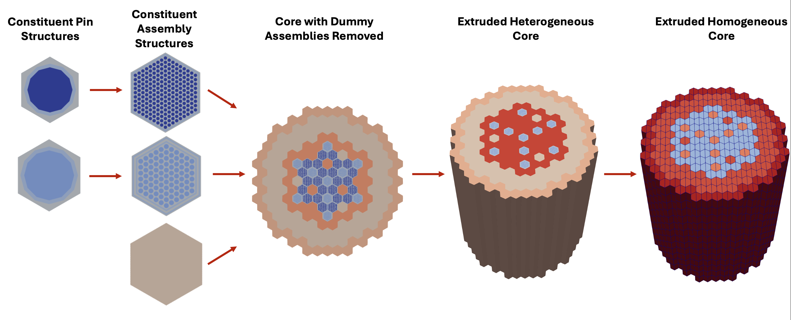
Output System
A system for outputting simulation data to the screen or files.
The output system is designed to be just like any other system in MOOSE: modular and expandable.
It is possible to create multiple output objects for outputting:
at specific time or timestep intervals,
custom subsets of variables, and
to various file types.
There exists a short-cut syntax for common output types as well as common parameters.
Short-cut Syntax
The following two methods for creating an Output object are equivalent within the internals of MOOSE.
[Outputs]
  exodus = true
[]
[Outputs]
  [out]
    type = Exodus
  []
[]
Customizing Output
The content of each Output can customized, see for example for an Exodus output:
[Outputs]
  [out]
    type = Exodus
    output_material_properties = true
    # removes some quantities from the output
    hide = 'power_pp pressure_var'
  []
[]
Common Parameters
[Outputs]
  interval = 10 # this is a time step interval
  [exo]
    type = Exodus
    interval = 1 # overrides interval from top-level
  []
  [cp]
    type = Checkpoint # Uses interval specified from top-level
  []
[]
Output Names
The default naming scheme for output files utilizes the input file name (e.g., input.i) with a suffix that differs depending on how the output is defined: An "_out" suffix is used for Outputs created using the short-cut syntax. sub-blocks use the actual sub-block name as the suffix.
[Outputs]
  exodus = true    # creates input_out.e
  [other]          # creates input_other.e
     type = Exodus
     interval = 2
  []
  [base]
    type = Exodus
    file_base = out # creates out.e
  []
[]
| Short-cut | Sub-block ("type=") | Description |
|---|---|---|
| console | Console | Writes to the screen and optionally a file |
| exodus | Exodus | The most common,well supported, and controllable output type |
| vtk | VTK | Visualization Toolkit format, requires --enable-vtk when building libMesh |
| gmv | GMV | General Mesh Viewer format |
| nemesis | Nemesis | Parallel ExodusII format |
| tecplot | Tecplot | Requires --enable-tecplot when building libMesh |
| xda | XDA | libMesh internal format (ascii) |
| xdr | XDR | libMesh internal format (binary) |
| csv | CSV | Comma separated scalar values |
| gnuplot | GNUPlot | Only support scalar outputs |
| checkpoint | Checkpoint | MOOSE internal format used for restart and recovery |
Paraview can read many of these (CSV, Exodus, Nemesis, VTK, GMV)
Step 3: Pressure Kernel with Material
Instead of passing constant parameters to the DarcyPressure object use the Material system to supply the values.
where is the permeability tensor and is the fluid viscosity.
This system allows for properties that vary in space and time, that can be coupled to variables in the simulation.
Material System
A system for defining material properties to be used by multiple systems and allow for variable coupling.
The material system operates by creating a producer/consumer relationship among objects
Materialobjects produce properties.Other MOOSE objects (including materials) consume these properties.
Producing Properties
Each property to be produced must be declared to be available for use, the
declareProperty<TYPE>()method does this and returns a writable reference.Override
computeQpProperties()to compute all of the declared properties at one quadrature point. Within this method, the references obtained from declaring the property are updated.
Consuming Properties
To consume a material property, call the correct get method in an object and store the constant reference as a member variable.
getMaterialProperty<TYPE>()
Use within non-AD objects to retrieve non-AD material properties.
getADMaterialProperty<TYPE>()
Use within AD objects to retrieve AD material properties.
Material Property Evaluation
Quantities are recomputed at quadrature points, as needed.
Multiple Material objects may define the same "property" for different parts of the subdomain or boundaries.
Stateful Material Properties
The values are not stored between timesteps unless "stateful" properties are enabled, which is accomplished by calling getMaterialPropertyOld<TYPE>() or getMaterialPropertyOlder<TYPE>()
It can be useful to have "old" values of Material properties available in a simulation, such as in solid mechanics plasticity constitutive models.
Traditionally, this type of value is called a "state variable"; in MOOSE, they are called "stateful material properties".
Stateful Material properties require more memory.
Default Material Properties
Default values for material properties may be assigned within the validParams function.
addParam<MaterialPropertyName>("combination_property_name", 12345,
 "The name of the property providing the luggage combination");
Only scalar (Real) values may have defaults.
When getMaterialProperty<Real>("combination_property_name") is called, the default will be returned if the value has not been computed via a declareProperty call within a Material object.
Material Property Output
Output of Material properties is enabled by setting the "outputs" parameter.
The following example creates additional variables called "real_property", "tensor_property", and "vector_property" that will show up in the output file.
[Materials<<<{"href": "../syntax/Materials/index.html"}>>>]
  [./hm]
    type = ParsedMaterial<<<{"description": "Parsed expression Material.", "href": "../source/materials/ParsedMaterial.html"}>>>
    property_name<<<{"description": "Name of the parsed material property"}>>> = hm
    coupled_variables<<<{"description": "Vector of variables used in the parsed function"}>>> = 'phi'
    expression<<<{"description": "Parsed function (see FParser) expression for the parsed material"}>>> = '3*phi^2 - 2*phi^3'
    outputs<<<{"description": "Vector of output names where you would like to restrict the output of variables(s) associated with this object"}>>> = exodus
  [../]
[]Supported Property Types for Output
Material properties can be of arbitrary (C++) type. Auxkernels have been created for material output only for specific common types:
| Type | AuxKernel | Variable Name(s) |
|---|---|---|
| Real | MaterialRealAux | prop |
| RealVectorValue | MaterialRealVectorValueAux | prop_1, prop_2, and prop_3 |
| RealTensorValue | MaterialRealTensorValueAux | prop_11, prop_12, prop_13, prop_21, etc. |
Function System
A system for defining analytic expressions based on the spatial location (, , ) and time, .
A Function object is created by inheriting from Function and overriding the virtual value() (and optionally other methods as well) functions.
Functions can be accessed in most MOOSE objects by calling getFunction("name"), where "name" matches a name from the input file.
A Function can depend an other functions, but not on material properties or variables.
Function Use
Many objects exist in MOOSE that utilize a function, such as:
FunctionDirichletBCFunctionNeumannBCFunctionICBodyForce
Each of these objects has a "function" parameter which is set in the input file, and controls which Function object is used.
Parsed Function
A ParsedFunction allow functions to be defined by strings directly in the input file, e.g.:
[Functions<<<{"href": "../syntax/Functions/index.html"}>>>]
  [sin_fn]
    type = ParsedFunction<<<{"description": "Function created by parsing a string", "href": "../source/functions/MooseParsedFunction.html"}>>>
    expression<<<{"description": "The user defined function."}>>> = sin(x)
  []
  [cos_fn]
    type = ParsedFunction<<<{"description": "Function created by parsing a string", "href": "../source/functions/MooseParsedFunction.html"}>>>
    expression<<<{"description": "The user defined function."}>>> = cos(x)
  []
  [fn]
    type = ParsedFunction<<<{"description": "Function created by parsing a string", "href": "../source/functions/MooseParsedFunction.html"}>>>
    # Inputs we will use in the parsed expression
    symbol_values<<<{"description": "Constant numeric values, postprocessor names, function names, and scalar variables corresponding to the symbols in symbol_names."}>>> = 'sin_fn cos_fn'
    # Short names for each input
    symbol_names<<<{"description": "Symbols (excluding t,x,y,z) that are bound to the values provided by the corresponding items in the symbol_values vector."}>>> = 's c'
    # Expression to parse
    expression<<<{"description": "The user defined function."}>>> = 's/c'
  []
[]It is possible to include other functions, as shown above, as well as scalar variables and postprocessor values with the function definition.
Default Functions
Whenever a Function object is added via addParam(), a default can be provided.
Both constant values and parsed function strings can be used as the default.
// Adding a Function with a default constant
params.addParam<FunctionName>("pressure_grad", "0.5", "The gradient of ...");

// Adding a Function with a default parsed function
params.addParam<FunctionName>("power_history", "t+100*sin(y)", "The power history of ...");
A ParsedFunction or ConstantFunction object is automatically constructed based on the default value if a function name is not supplied in the input file.
Step 3: Pressure Kernel with Material
(continued)
PackedColumn Material
Two material properties must be produced for consumption by DarcyPressure object: permeability and viscosity.
Both shall be computed with a single Material object: PackedColumn.
As in the reference article, permeability varies with the size of the steel spheres, so we'll perform an interpolation calculation for it over the range of valid values.
PackedColumn.h
#pragma once

#include "Material.h"

/**
 * Material objects inherit from Material and override computeQpProperties.
 *
 * Their job is to declare properties for use by other objects in the
 * calculation such as Kernels and BoundaryConditions.
 */
class PackedColumn : public Material
{
public:
  static InputParameters validParams();

  PackedColumn(const InputParameters & parameters);

protected:
  /// Necessary override. This is where the values of the properties are computed.
  virtual void computeQpProperties() override;

  /// The radius of the spheres in the column
  const Function & _input_radius;

  /// Value of viscosity from the input file
  const Real & _input_viscosity;

  /// The permeability (K) computed based on the radius (mm)
  ADMaterialProperty<Real> & _permeability;

  /// The viscosity of the fluid (mu)
  ADMaterialProperty<Real> & _viscosity;
};
PackedColumn.C
#include "PackedColumn.h"
#include "Function.h"

registerMooseObject("DarcyThermoMechApp", PackedColumn);

InputParameters
PackedColumn::validParams()
{
  InputParameters params = Material::validParams();

  // Parameter for radius of the spheres used to interpolate permeability.
  params.addParam<FunctionName>("radius",
                                "1.0",
                                "The radius of the steel spheres (mm) that are packed in the "
                                "column for computing permeability.");
  params.addParam<Real>(
      "viscosity",
      7.98e-4,
      "The viscosity ($\\mu$) of the fluid in Pa, the default is for water at 30 degrees C.");

  return params;
}

PackedColumn::PackedColumn(const InputParameters & parameters)
  : Material(parameters),

    // Get the parameters from the input file
    _input_radius(getFunction("radius")),
    _input_viscosity(getParam<Real>("viscosity")),

    // Material Properties being produced by this object
    _permeability(declareADProperty<Real>("permeability")),
    _viscosity(declareADProperty<Real>("viscosity"))
{
}

void
PackedColumn::computeQpProperties()
{
  // From the paper: Table 1
  std::vector<Real> sphere_sizes = {1, 3};
  std::vector<Real> permeability = {0.8451e-9, 8.968e-9};

  Real value = _input_radius.value(_t, _q_point[_qp]);
  mooseAssert(value >= 1 && value <= 3,
              "The radius range must be in the range [1, 3], but " << value << " provided.");

  _viscosity[_qp] = _input_viscosity;

  // We'll calculate permeability using a simple linear interpolation of the two points above:
  //          y0 * (x1 - x) + y1 * (x - x0)
  //  y(x) = -------------------------------
  //                     x1 - x0
  _permeability[_qp] =
      (permeability[0] * (sphere_sizes[1] - value) + permeability[1] * (value - sphere_sizes[0])) /
      (sphere_sizes[1] - sphere_sizes[0]);
}
DarcyPressure Kernel
The existing Kernel object uses input parameters for defining permeability and viscosity, it must be updated to consume the newly created material properties.
DarcyPressure.h
 @@ -1,24 +1,32 @@

 #pragma once

 // Including the "ADKernel" Kernel here so we can extend it
 #include "ADKernel.h"

 /**
  * Computes the residual contribution: K / mu * grad_u * grad_phi.
  */
 class DarcyPressure : public ADKernel
 {
 public:
   static InputParameters validParams();

   DarcyPressure(const InputParameters & parameters);

 protected:
   /// ADKernel objects must override precomputeQpResidual
   virtual ADReal computeQpResidual() override;

-  /// References to be set from input file
-  const Real & _permeability;
-  const Real & _viscosity;
+  // References to be set from Material system
+
+  /// The viscosity. This is declared as an \p ADMaterialProperty, meaning any derivative
+  /// information coming from the producing \p Material will be preserved and the integrity of the
+  /// non-linear solve will be likewise preserved
+  const ADMaterialProperty<Real> & _permeability;
+
+  /// The viscosity. This is declared as an \p ADMaterialProperty, meaning any derivative
+  /// information coming from the producing \p Material will be preserved and the integrity of the
+  /// non-linear solve will be likewise preserved
+  const ADMaterialProperty<Real> & _viscosity;
 };
(+ tutorials/darcy_thermo_mech/step03_darcy_material/include/kernels/DarcyPressure.h)
DarcyPressure.C
 @@ -1,37 +1,26 @@

 #include "DarcyPressure.h"

 registerMooseObject("DarcyThermoMechApp", DarcyPressure);

 InputParameters
 DarcyPressure::validParams()
 {
   InputParameters params = ADKernel::validParams();
   params.addClassDescription("Compute the diffusion term for Darcy pressure ($p$) equation: "
                              "$-\\nabla \\cdot \\frac{\\mathbf{K}}{\\mu} \\nabla p = 0$");
-
-  // Add a required parameter.  If this isn't provided in the input file MOOSE will error.
-  params.addRequiredParam<Real>("permeability", "The permeability ($\\mathrm{K}$) of the fluid.");
-
-  // Add a parameter with a default value; this value can be overridden in the input file.
-  params.addParam<Real>(
-      "viscosity",
-      7.98e-4,
-      "The viscosity ($\\mu$) of the fluid in Pa, the default is for water at 30 degrees C.");
   return params;
 }

 DarcyPressure::DarcyPressure(const InputParameters & parameters)
   : ADKernel(parameters),
-
-    // Get the parameters from the input file
-    _permeability(getParam<Real>("permeability")),
-    _viscosity(getParam<Real>("viscosity"))
+    _permeability(getADMaterialProperty<Real>("permeability")),
+    _viscosity(getADMaterialProperty<Real>("viscosity"))
 {
 }

 ADReal
 DarcyPressure::computeQpResidual()
 {
-  return (_permeability / _viscosity) * _grad_test[_i][_qp] * _grad_u[_qp];
+  return (_permeability[_qp] / _viscosity[_qp]) * _grad_test[_i][_qp] * _grad_u[_qp];
 }
(+ tutorials/darcy_thermo_mech/step03_darcy_material/src/kernels/DarcyPressure.C)
Step 3: Input File
 @@ -1,52 +1,55 @@
 [Mesh<<<{"href": "../syntax/Mesh/index.html"}>>>]
   [gmg]
     type = GeneratedMeshGenerator<<<{"description": "Create a line, square, or cube mesh with uniformly spaced or biased elements.", "href": "../source/meshgenerators/GeneratedMeshGenerator.html"}>>> # Can generate simple lines, rectangles and rectangular prisms
     dim<<<{"description": "The dimension of the mesh to be generated"}>>> = 2                       # Dimension of the mesh
     nx<<<{"description": "Number of elements in the X direction"}>>> = 100                      # Number of elements in the x direction
     ny<<<{"description": "Number of elements in the Y direction"}>>> = 10                       # Number of elements in the y direction
     xmax<<<{"description": "Upper X Coordinate of the generated mesh"}>>> = 0.304                  # Length of test chamber
     ymax<<<{"description": "Upper Y Coordinate of the generated mesh"}>>> = 0.0257                 # Test chamber radius
   []
   coord_type = RZ                 # Axisymmetric RZ
   rz_coord_axis = X               # Which axis the symmetry is around
 []

 [Variables<<<{"href": "../syntax/Variables/index.html"}>>>/pressure]
   # Adds a Linear Lagrange variable by default
 []

 [Kernels<<<{"href": "../syntax/Kernels/index.html"}>>>/darcy_pressure]
   type = DarcyPressure
   variable = pressure
-  permeability = 0.8451e-9 # (m^2) 1mm spheres.
 []

 [BCs<<<{"href": "../syntax/BCs/index.html"}>>>]
   [inlet]
     type = DirichletBC<<<{"description": "Imposes the essential boundary condition $u=g$, where $g$ is a constant, controllable value.", "href": "../source/bcs/DirichletBC.html"}>>>  # Simple u=value BC
     variable<<<{"description": "The name of the variable that this residual object operates on"}>>> = pressure # Variable to be set
     boundary<<<{"description": "The list of boundary IDs from the mesh where this object applies"}>>> = left     # Name of a sideset in the mesh
     value<<<{"description": "Value of the BC"}>>> = 4000        # (Pa) From Figure 2 from paper.  First data point for 1mm spheres.
   []
   [outlet]
     type = DirichletBC<<<{"description": "Imposes the essential boundary condition $u=g$, where $g$ is a constant, controllable value.", "href": "../source/bcs/DirichletBC.html"}>>>
     variable<<<{"description": "The name of the variable that this residual object operates on"}>>> = pressure
     boundary<<<{"description": "The list of boundary IDs from the mesh where this object applies"}>>> = right
     value<<<{"description": "Value of the BC"}>>> = 0           # (Pa) Gives the correct pressure drop from Figure 2 for 1mm spheres
   []
 []

+[Materials<<<{"href": "../syntax/Materials/index.html"}>>>/column]
+  type = PackedColumn
+[]
+
 [Problem<<<{"href": "../syntax/Problem/index.html"}>>>]
   type = FEProblem  # This is the "normal" type of Finite Element Problem in MOOSE
 []

 [Executioner<<<{"href": "../syntax/Executioner/index.html"}>>>]
   type = Steady       # Steady state problem
   solve_type = NEWTON # Perform a Newton solve, uses AD to compute Jacobian terms
   petsc_options_iname = '-pc_type -pc_hypre_type' # PETSc option pairs with values below
   petsc_options_value = 'hypre boomeramg'
 []

 [Outputs<<<{"href": "../syntax/Outputs/index.html"}>>>]
   exodus<<<{"description": "Output the results using the default settings for Exodus output."}>>> = true # Output Exodus format
[](+ tutorials/darcy_thermo_mech/step03_darcy_material/problems/step3.i)
Step 3: Run
cd ~/projects/moose/tutorials/darcy_thermo_mech/step03_darcy_material
make -j 12 # use number of processors for your system
cd problems
../darcy_thermo_mech-opt -i step3.i
Step 3: Result

Step 3b: Variable Spheres
Update the input file to vary the sphere size from 1 to 3 along the length of the pipe.
Step 3b: Input File
 @@ -1,55 +1,57 @@
 [Mesh<<<{"href": "../syntax/Mesh/index.html"}>>>]
   [gmg]
     type = GeneratedMeshGenerator<<<{"description": "Create a line, square, or cube mesh with uniformly spaced or biased elements.", "href": "../source/meshgenerators/GeneratedMeshGenerator.html"}>>> # Can generate simple lines, rectangles and rectangular prisms
     dim<<<{"description": "The dimension of the mesh to be generated"}>>> = 2                       # Dimension of the mesh
     nx<<<{"description": "Number of elements in the X direction"}>>> = 100                      # Number of elements in the x direction
     ny<<<{"description": "Number of elements in the Y direction"}>>> = 10                       # Number of elements in the y direction
     xmax<<<{"description": "Upper X Coordinate of the generated mesh"}>>> = 0.304                  # Length of test chamber
     ymax<<<{"description": "Upper Y Coordinate of the generated mesh"}>>> = 0.0257                 # Test chamber radius
   []
   coord_type = RZ                 # Axisymmetric RZ
   rz_coord_axis = X               # Which axis the symmetry is around
 []

 [Variables<<<{"href": "../syntax/Variables/index.html"}>>>/pressure]
   # Adds a Linear Lagrange variable by default
 []

 [Kernels<<<{"href": "../syntax/Kernels/index.html"}>>>/darcy_pressure]
   type = DarcyPressure
   variable = pressure
 []

 [BCs<<<{"href": "../syntax/BCs/index.html"}>>>]
   [inlet]
     type = DirichletBC<<<{"description": "Imposes the essential boundary condition $u=g$, where $g$ is a constant, controllable value.", "href": "../source/bcs/DirichletBC.html"}>>>  # Simple u=value BC
     variable<<<{"description": "The name of the variable that this residual object operates on"}>>> = pressure # Variable to be set
     boundary<<<{"description": "The list of boundary IDs from the mesh where this object applies"}>>> = left     # Name of a sideset in the mesh
     value<<<{"description": "Value of the BC"}>>> = 4000        # (Pa) From Figure 2 from paper.  First data point for 1mm spheres.
   []
   [outlet]
     type = DirichletBC<<<{"description": "Imposes the essential boundary condition $u=g$, where $g$ is a constant, controllable value.", "href": "../source/bcs/DirichletBC.html"}>>>
     variable<<<{"description": "The name of the variable that this residual object operates on"}>>> = pressure
     boundary<<<{"description": "The list of boundary IDs from the mesh where this object applies"}>>> = right
     value<<<{"description": "Value of the BC"}>>> = 0           # (Pa) Gives the correct pressure drop from Figure 2 for 1mm spheres
   []
 []

 [Materials<<<{"href": "../syntax/Materials/index.html"}>>>/column]
   type = PackedColumn
+  radius = '1 + 2/3.04*x'
+  outputs = exodus
 []

 [Problem<<<{"href": "../syntax/Problem/index.html"}>>>]
   type = FEProblem  # This is the "normal" type of Finite Element Problem in MOOSE
 []

 [Executioner<<<{"href": "../syntax/Executioner/index.html"}>>>]
   type = Steady       # Steady state problem
   solve_type = NEWTON # Perform a Newton solve, uses AD to compute Jacobian terms
   petsc_options_iname = '-pc_type -pc_hypre_type' # PETSc option pairs with values below
   petsc_options_value = 'hypre boomeramg'
 []

 [Outputs<<<{"href": "../syntax/Outputs/index.html"}>>>]
   exodus<<<{"description": "Output the results using the default settings for Exodus output."}>>> = true # Output Exodus format
[](+ tutorials/darcy_thermo_mech/step03_darcy_material/problems/step3b.i)
Step 3b: Result

Test System
Continuous Integration
Continuous integration is a software development practice where developers regularly merge their code changes into a central repository, after which automated builds and tests are run. The key goals of continuous integration are to find and address bugs quicker, improve software quality, and reduce the time it takes to validate and release new software updates.
Testing enables continuous integration by ensuring your changes do not break previous capabilities of the code.
Overview
MOOSE includes an extendable test system (python) for executing code with different input files.
Each kernel (or logical set of kernels) should have test(s) for verification.
The test system is flexible, it performs many different operations such as testing for expected error conditions.
Additionally, custom "Tester" objects can be created.
Test Setup
Related tests should be grouped into an individual directory and have a consistent naming convention.
It is recommended to organize tests in a hierarchy similar to the application source (i.e., kernels, BCs, materials, etc).
Tests are found dynamically by matching patterns (highlighted below)
tests/
  kernels/
    my_kernel_test/
      my_kernel_test.e   [input mesh]
      my_kernel_test.i   [input file]
      tests              [test specification file]
      gold/              [gold standard folder for validated solution]
        out.e            [solution]
Test Specification
Test specifications use the hit format, the same format as the standard MOOSE input file.
[Tests]
   [my_kernel_test]
     type    = Exodiff
     input   = my_kernel_test.i
     exodiff = my_kernel_test_out.e
   []

   [kernel_check_exception]
     type       = RunException
     input      = my_kernel_exception.i
     expect_err = 'Bad stuff happened with variable \w+'
   []
 []
Test Objects
RunApp: Runs a MOOSE-based application with specified options
Exodiff: Checks Exodus files for differences within specified tolerances
CSVDiff: Checks CSV files for differences within specified tolerances
VTKDiff: Checks VTK files for differences within specified tolerances
RunException: Tests for error conditions
CheckFiles: Checks for the existence of specific files after a completed run
ImageDiff: Compares images (e.g., *.png) for differences within specified tolerances
PythonUnitTest: Runs python "unittest" based tests
AnalyzeJacobian: Compares computed Jacobian with finite difference version
PetscJacobianTester: Compares computed Jacobian using PETSc
Running Tests
./run_tests -j 12
For more information view the help:
./run_tests -h
Test Object Options
./run_tests --dump
input: The name of the input file
exodiff: The list of output filenames to compare
abs_zero: Absolute zero tolerance for exodiff
rel_err: Relative error tolerance for exodiff
prereq: Name of the test that needs to complete before running this test
min_parallel: Minimum number of processors to use for a test (default: 1)
max_parallel: Maximum number of processors to use for a test
Notes on Tests
Individual tests should run relatively quickly (2 second rule)
Outputs or other generated files should not be checked into the repository
MOOSE developers rely on application tests when refactoring to verify correctness
poor test coverage = higher code failure rate
Step 4: Velocity Auxiliary Variable
The velocity is the primary variable of interest, it is computed based on the pressure as:
Auxiliary System
A system for direct calculation of field variables ("AuxVariables") that is designed for postprocessing, coupling, and proxy calculations.
The term "nonlinear variable" is defined, in MOOSE language, as a variable that is being solved for using a nonlinear system of PDEs using Kernel and BoundaryCondition objects.
The term "auxiliary variable" is defined, in MOOSE language, as a variable that is directly calculated using an AuxKernel object.
AuxVariables
Auxiliary variables are declared in the [AuxVariables] input file block
Auxiliary variables are field variables that are associated with finite element shape functions and can serve as a proxy for nonlinear variables
Auxiliary variables currently come in two flavors:
Element (e.g. constant or higher order monomials)
Nodal (e.g. linear Lagrange)
Auxiliary variables have "old" and "older" states, from previous time steps, just like nonlinear variables
Elemental Auxiliary Variables
Element auxiliary variables can compute:
average values per element, if stored in a constant monomial variable
spatial profiles using higher order variables
AuxKernel objects computing elemental values can couple to nonlinear variables and both element and nodal auxiliary variables
[AuxVariables]
  [aux]
    order = CONSTANT
    family = MONOMIAL
  []
[]
Nodal Auxiliary Variables
Nodal auxiliary variables are computed at each node and are stored as linear Lagrange variables
AuxKernel objects computing nodal values can only couple to nodal nonlinear variables and other nodal auxiliary variables
[AuxVariables]
  [aux]
    order = LAGRANGE
    family = FIRST
  []
[]
AuxKernel Objects
Directly compute AuxVariable values by overriding computeValue() and they can operate on both elemental and nodal auxiliary variable.
When operating on a nodal variable computeValue() operates on each node; when operating on a elemental variable it operates on each element.
AuxKernel Object Members
_u, _grad_u
Value and gradient of variable this AuxKernel is operating on
_q_point
Coordinates of the current q-point that is only valid for elemental AuxKernels, _current_node should be used for nodal variables
_qp
Current quadrature point, this indexing is used for both nodal (_qp=0 at the node) and elemental variables for consistency
_current_elem
Pointer to the current element that is being operated on (elemental only)
_current_node
Pointer to the current node that is being operated on (nodal only)
VectorAuxKernel Objects
Directly compute a vector AuxVariable values by:
inheriting from the
VectorAuxKernelclassoverriding
computeValue(), with the difference being the return value of aRealVectorValueinstead of Real.
The auxiliary variable will have to be one of the vector types (LAGRANCE_VEC, MONOMIAL_VEC or NEDELEC_VEC).
[AuxVariables]
  [aux]
    order = FIRST
    family = LAGRANGE_VEC
  []
[]
[AuxKernels]
  [parsed]
    type = ParsedVectorAux
    variable = aux
    expression_x = 'x + y'
    expression_y = 'x - y'
  []
[]
Step 4: Velocity Auxiliary Variable
(continued)
DarcyVelocity AuxKernel
The primary unknown ("nonlinear variable") is the pressure
Once the pressure is computed, the AuxiliarySystem can compute and output the velocity field using the coupled pressure variable and the permeability and viscosity properties.
Auxiliary variables come in two flavors: Nodal and Elemental.
Nodal auxiliary variables cannot couple to gradients of nonlinear variables since gradients of continuous variables are not well-defined at the nodes.
Elemental auxiliary variables can couple to gradients of nonlinear variables since evaluation occurs in the element interiors.
DarcyVelocity.h
#pragma once

#include "AuxKernel.h"

/**
 * Auxiliary kernel responsible for computing the Darcy velocity given
 * several fluid properties and the pressure gradient.
 */
class DarcyVelocity : public VectorAuxKernel
{
public:
  static InputParameters validParams();

  DarcyVelocity(const InputParameters & parameters);

protected:
  /**
   * AuxKernels MUST override computeValue.  computeValue() is called on
   * every quadrature point.  For Nodal Auxiliary variables those quadrature
   * points coincide with the nodes.
   */
  virtual RealVectorValue computeValue() override;

  /// The gradient of a coupled variable
  const VariableGradient & _pressure_gradient;

  /// Holds the permeability and viscosity from the material system
  const ADMaterialProperty<Real> & _permeability;
  const ADMaterialProperty<Real> & _viscosity;
};
DarcyVelocity.C
#include "DarcyVelocity.h"

#include "metaphysicl/raw_type.h"

registerMooseObject("DarcyThermoMechApp", DarcyVelocity);

InputParameters
DarcyVelocity::validParams()
{
  InputParameters params = VectorAuxKernel::validParams();

  // Add a "coupling paramater" to get a variable from the input file.
  params.addRequiredCoupledVar("pressure", "The pressure field.");

  return params;
}

DarcyVelocity::DarcyVelocity(const InputParameters & parameters)
  : VectorAuxKernel(parameters),

    // Get the gradient of the variable
    _pressure_gradient(coupledGradient("pressure")),

    // Set reference to the permeability MaterialProperty.
    // Only AuxKernels operating on Elemental Auxiliary Variables can do this
    _permeability(getADMaterialProperty<Real>("permeability")),

    // Set reference to the viscosity MaterialProperty.
    // Only AuxKernels operating on Elemental Auxiliary Variables can do this
    _viscosity(getADMaterialProperty<Real>("viscosity"))
{
}

RealVectorValue
DarcyVelocity::computeValue()
{
  // Access the gradient of the pressure at this quadrature point, then pull out the "component" of
  // it requested (x, y or z). Note, that getting a particular component of a gradient is done using
  // the parenthesis operator.
  return -MetaPhysicL::raw_value(_permeability[_qp] / _viscosity[_qp]) * _pressure_gradient[_qp];
}
Step 4: Input File
 @@ -1,55 +1,70 @@
 [Mesh<<<{"href": "../syntax/Mesh/index.html"}>>>]
   [gmg]
     type = GeneratedMeshGenerator<<<{"description": "Create a line, square, or cube mesh with uniformly spaced or biased elements.", "href": "../source/meshgenerators/GeneratedMeshGenerator.html"}>>> # Can generate simple lines, rectangles and rectangular prisms
     dim<<<{"description": "The dimension of the mesh to be generated"}>>> = 2                       # Dimension of the mesh
     nx<<<{"description": "Number of elements in the X direction"}>>> = 100                      # Number of elements in the x direction
     ny<<<{"description": "Number of elements in the Y direction"}>>> = 10                       # Number of elements in the y direction
     xmax<<<{"description": "Upper X Coordinate of the generated mesh"}>>> = 0.304                  # Length of test chamber
     ymax<<<{"description": "Upper Y Coordinate of the generated mesh"}>>> = 0.0257                 # Test chamber radius
   []
   coord_type = RZ                 # Axisymmetric RZ
   rz_coord_axis = X               # Which axis the symmetry is around
 []

 [Variables<<<{"href": "../syntax/Variables/index.html"}>>>/pressure]
   # Adds a Linear Lagrange variable by default
 []

+[AuxVariables<<<{"href": "../syntax/AuxVariables/index.html"}>>>/velocity]
+  order<<<{"description": "Specifies the order of the FE shape function to use for this variable (additional orders not listed are allowed)"}>>> = CONSTANT
+  family<<<{"description": "Specifies the family of FE shape functions to use for this variable"}>>> = MONOMIAL_VEC
+[]
+
 [Kernels<<<{"href": "../syntax/Kernels/index.html"}>>>/darcy_pressure]
   type = DarcyPressure
   variable = pressure
+[]
+
+[AuxKernels<<<{"href": "../syntax/AuxKernels/index.html"}>>>]
+  [velocity]
+    type = DarcyVelocity
+    variable = velocity
+    execute_on = timestep_end
+    pressure = pressure
+  []
 []

 [BCs<<<{"href": "../syntax/BCs/index.html"}>>>]
   [inlet]
     type = DirichletBC<<<{"description": "Imposes the essential boundary condition $u=g$, where $g$ is a constant, controllable value.", "href": "../source/bcs/DirichletBC.html"}>>>  # Simple u=value BC
     variable<<<{"description": "The name of the variable that this residual object operates on"}>>> = pressure # Variable to be set
     boundary<<<{"description": "The list of boundary IDs from the mesh where this object applies"}>>> = left     # Name of a sideset in the mesh
     value<<<{"description": "Value of the BC"}>>> = 4000        # (Pa) From Figure 2 from paper.  First data point for 1mm spheres.
   []
   [outlet]
     type = DirichletBC<<<{"description": "Imposes the essential boundary condition $u=g$, where $g$ is a constant, controllable value.", "href": "../source/bcs/DirichletBC.html"}>>>
     variable<<<{"description": "The name of the variable that this residual object operates on"}>>> = pressure
     boundary<<<{"description": "The list of boundary IDs from the mesh where this object applies"}>>> = right
     value<<<{"description": "Value of the BC"}>>> = 0           # (Pa) Gives the correct pressure drop from Figure 2 for 1mm spheres
   []
 []

 [Materials<<<{"href": "../syntax/Materials/index.html"}>>>/column]
   type = PackedColumn
+  radius = 1
 []

 [Problem<<<{"href": "../syntax/Problem/index.html"}>>>]
   type = FEProblem  # This is the "normal" type of Finite Element Problem in MOOSE
 []

 [Executioner<<<{"href": "../syntax/Executioner/index.html"}>>>]
   type = Steady       # Steady state problem
   solve_type = NEWTON # Perform a Newton solve, uses AD to compute Jacobian terms
   petsc_options_iname = '-pc_type -pc_hypre_type' # PETSc option pairs with values below
   petsc_options_value = 'hypre boomeramg'
 []

 [Outputs<<<{"href": "../syntax/Outputs/index.html"}>>>]
   exodus<<<{"description": "Output the results using the default settings for Exodus output."}>>> = true # Output Exodus format
[](+ tutorials/darcy_thermo_mech/step04_velocity_aux/problems/step4.i)
Step 4: Run
cd ~/projects/moose/tutorials/darcy_thermo_mech/step04_velocity_aux
make -j 12 # use number of processors for your system
cd problems
../darcy_thermo_mech-opt -i step4.i
Step 4: Result

Tighter Solve Tolerance
cd ~/projects/moose/tutorials/darcy_thermo_mech/step04_velocity_aux
make -j 12 # use number of processors for your system
cd problems
../darcy_thermo_mech-opt -i step4.i Executioner/nl_rel_tol=1e-12

Step 5: Heat Conduction
With the pressure equation handled, the heat conduction equation is next.
Initially, only the steady heat conduction equation is considered:
This is another diffusion-type term that depends on the thermal conductivity, . This term is implemented in the MOOSE heat transfer module as ADHeatConduction.
ADHeatConduction.h
#pragma once

#include "ADDiffusion.h"

class ADHeatConduction : public ADDiffusion
{
public:
  static InputParameters validParams();

  ADHeatConduction(const InputParameters & parameters);

protected:
  virtual ADRealVectorValue precomputeQpResidual() override;

  const ADMaterialProperty<Real> & _thermal_conductivity;
};
ADHeatConduction.C
#include "ADHeatConduction.h"

registerMooseObject("HeatTransferApp", ADHeatConduction);

InputParameters
ADHeatConduction::validParams()
{
  InputParameters params = ADDiffusion::validParams();
  params.addParam<MaterialPropertyName>("thermal_conductivity",
                                        "thermal_conductivity",
                                        "the name of the thermal conductivity material property");
  params.set<bool>("use_displaced_mesh") = true;
  return params;
}

ADHeatConduction::ADHeatConduction(const InputParameters & parameters)
  : ADDiffusion(parameters),
    _thermal_conductivity(getADMaterialProperty<Real>("thermal_conductivity"))
{
}

ADRealVectorValue
ADHeatConduction::precomputeQpResidual()
{
  return _thermal_conductivity[_qp] * ADDiffusion::precomputeQpResidual();
}
The ADHeatConduction Kernel in conjunction with a GenericConstantMaterial is all that is needed to perform a steady state heat conduction solve (with at the inlet and at the outlet).
GenericConstantMaterial
GenericConstantMaterial is a simple way to define constant material properties.
Two input parameters are provided using "list" syntax common to MOOSE:
[Materials/material]
  type = GenericConstantMaterial
  prop_names  = 'conductivity density'
  prop_values = '0.01         200'
[]
Step 5a: Steady-State Input File
[Mesh<<<{"href": "../syntax/Mesh/index.html"}>>>]
  [gmg]
    type = GeneratedMeshGenerator<<<{"description": "Create a line, square, or cube mesh with uniformly spaced or biased elements.", "href": "../source/meshgenerators/GeneratedMeshGenerator.html"}>>>
    dim<<<{"description": "The dimension of the mesh to be generated"}>>> = 2
    nx<<<{"description": "Number of elements in the X direction"}>>> = 100
    ny<<<{"description": "Number of elements in the Y direction"}>>> = 10
    xmax<<<{"description": "Upper X Coordinate of the generated mesh"}>>> = 0.304 # Length of test chamber
    ymax<<<{"description": "Upper Y Coordinate of the generated mesh"}>>> = 0.0257 # Test chamber radius
  []
  coord_type = RZ
  rz_coord_axis = X
[]

[Variables<<<{"href": "../syntax/Variables/index.html"}>>>]
  [temperature]
  []
[]

[Kernels<<<{"href": "../syntax/Kernels/index.html"}>>>]
  [heat_conduction]
    type = ADHeatConduction<<<{"description": "Same as `Diffusion` in terms of physics/residual, but the Jacobian is computed using forward automatic differentiation", "href": "../source/kernels/ADHeatConduction.html"}>>>
    variable<<<{"description": "The name of the variable that this residual object operates on"}>>> = temperature
  []
[]

[BCs<<<{"href": "../syntax/BCs/index.html"}>>>]
  [inlet_temperature]
    type = DirichletBC<<<{"description": "Imposes the essential boundary condition $u=g$, where $g$ is a constant, controllable value.", "href": "../source/bcs/DirichletBC.html"}>>>
    variable<<<{"description": "The name of the variable that this residual object operates on"}>>> = temperature
    boundary<<<{"description": "The list of boundary IDs from the mesh where this object applies"}>>> = left
    value<<<{"description": "Value of the BC"}>>> = 350 # (K)
  []
  [outlet_temperature]
    type = DirichletBC<<<{"description": "Imposes the essential boundary condition $u=g$, where $g$ is a constant, controllable value.", "href": "../source/bcs/DirichletBC.html"}>>>
    variable<<<{"description": "The name of the variable that this residual object operates on"}>>> = temperature
    boundary<<<{"description": "The list of boundary IDs from the mesh where this object applies"}>>> = right
    value<<<{"description": "Value of the BC"}>>> = 300 # (K)
  []
[]

[Materials<<<{"href": "../syntax/Materials/index.html"}>>>/steel]
  type = ADGenericConstantMaterial<<<{"description": "Declares material properties based on names and values prescribed by input parameters.", "href": "../source/materials/GenericConstantMaterial.html"}>>>
  prop_names<<<{"description": "The names of the properties this material will have"}>>> = thermal_conductivity
  prop_values<<<{"description": "The values associated with the named properties"}>>> = 18 # K: (W/m*K) from wikipedia @296K
[]

[Problem<<<{"href": "../syntax/Problem/index.html"}>>>]
  type = FEProblem
[]

[Executioner<<<{"href": "../syntax/Executioner/index.html"}>>>]
  type = Steady
  solve_type = NEWTON
  petsc_options_iname = '-pc_type -pc_hypre_type'
  petsc_options_value = 'hypre boomeramg'
[]

[Outputs<<<{"href": "../syntax/Outputs/index.html"}>>>]
  exodus<<<{"description": "Output the results using the default settings for Exodus output."}>>> = true
[]Step 5a: Running Input File
cd ~/projects/moose/tutorials/darcy_thermo_mech/step5_heat_conduction
make -j 12 # use number of processors for your system
cd problems
../darcy_thermo_mech-opt -i step5a_steady.i
Transient Heat Conduction (5b)
To create a time-dependent problem add in the time derivative:
The time term exists in the heat transfer module as ADHeatConductionTimeDerivative, thus only an update to the input file is required to run the transient case.
Executioner System
A system for dictating the simulation solving strategy.
Steady-state Executioner
Steady-state executioners generally solve the nonlinear system just once.
[Executioner<<<{"href": "../syntax/Executioner/index.html"}>>>]
  type = Steady
[]The Steady executioner can solve the nonlinear system multiple times while adaptively refining the mesh to improve the solution.
Transient Executioners
Transient executioners solve the nonlinear system at least once per time step.
| Option | Definition |
|---|---|
dt | Starting time step size |
num_steps | Number of time steps |
start_time | The start time of the simulation |
end_time | The end time of the simulation |
scheme | Time integration scheme (discussed next) |
[Executioner<<<{"href": "../syntax/Executioner/index.html"}>>>]
  type = Transient
  scheme = 'implicit-euler'
  solve_type = 'PJFNK'
  start_time = 0.0
  num_steps = 5
  dt = 0.1
[]Steady-State Detection
| Option | Definition |
|---|---|
steady_state_detection | Whether to try and detect achievement of steady-state (Default = false) |
steady_state_tolerance | Used for determining a steady-state; Compared against the difference in solution vectors between current and old time steps (Default = 1e-8) |
Common Executioner Options
There are a number of options that appear in the executioner block and are used to control the solver. Here are a few common options:
| Option | Definition |
|---|---|
l_tol | Linear Tolerance (default: 1e-5) |
l_max_its | Max Linear Iterations (default: 10000) |
nl_rel_tol | Nonlinear Relative Tolerance (default: 1e-8) |
nl_abs_tol | Nonlinear Absolute Tolerance (default: 1e-50) |
nl_max_its | Max Nonlinear Iterations (default: 50) |
TimeKernel Object
The TimeKernel object adds two member variables to a Kernel object:
_u_dot
Time derivative of the associated nonlinear variable
_du_dot_du
The derivative of _u_dot with respect to _u
TimeKernel Base Classes
| Base | Override | Use |
|---|---|---|
| TimeKernel ADTimeKernel | computeQpResidual | Use when the time term in the PDE is multiplied by both the test function and the gradient of the test function (_test and _grad_test must be applied) |
| TimeKernelValue ADTimeKernelValue | precomputeQpResidual | Use when the time term computed in the PDE is only multiplied by the test function (do not use _test in the override, it is applied automatically) |
| TimeKernelGrad ADTimeKernelGrad | precomputeQpResidual | Use when the time term computed in the PDE is only multiplied by the gradient of the test function (do not use _grad_test in the override, it is applied automatically) |
Time Integrator System
A system for defining schemes for numerical integration in time.
The TimeIntegrator can be set using "scheme" parameter within the [Executioner] block, if the "type = Transient", the following options exist:
implicit-euler: Backward Euler (default)bdf2: Second order backward difference formulacrank-nicolson: Second order Crank-Nicolson methoddirk: Second order Diagonally-Implicit Runge-Kutta (DIRK)newmark-beta: Second order Newmark-beta method (structural dynamics)
TimeIntegrator Block
It is also possible to specify a time integrator as a separate sub-block within the input file. This allows for additional types and parameters to be defined, including custom TimeIntegrator objects.
[Executioner<<<{"href": "../syntax/Executioner/index.html"}>>>]
  type = Transient
  start_time = 0.0
  num_steps = 6
  dt = 0.1
  [TimeIntegrator<<<{"href": "../syntax/Executioner/TimeIntegrator/index.html"}>>>]
    type = NewmarkBeta
    beta = 0.4225
    gamma = 0.8
  []
[]Convergence Rates
Consider the test problem:
for , and , is chosen so the exact solution is given by and and are the initial and Dirichlet boundary conditions corresponding to this exact solution.

Time Stepper System
A system for suggesting time steps for transient executioners.
[Executioner<<<{"href": "../syntax/Executioner/index.html"}>>>]
  type = Transient
  end_time = 20.0
  verbose = true

  [TimeStepper<<<{"href": "../syntax/Executioner/TimeStepper/index.html"}>>>]
    type = IterationAdaptiveDT
    dt = 1.0
    optimal_iterations = 10
    time_t = '0.0 5.0'
    time_dt = '1.0 5.0'
  []
[]Custom objects are created by inheriting from TimeStepper overriding computeDT().
Built-in TimeSteppers
MOOSE includes many built-in TimeStepper objects:
ConstantDTIterationAdaptiveDTFunctionDTPostprocessorDTFixedPointIterationAdaptiveDTTimeSequenceStepper
IterationAdaptiveDT
IterationAdaptiveDT grows or shrinks the time step based on the number of iterations taken to obtain a converged solution in the last converged step.
[Executioner<<<{"href": "../syntax/Executioner/index.html"}>>>]
  type = Transient
  solve_type = NEWTON
  start_time = 0.0
  dtmin = 1.0
  end_time = 10.0
  [TimeStepper<<<{"href": "../syntax/Executioner/TimeStepper/index.html"}>>>]
    type = IterationAdaptiveDT
    optimal_iterations = 1
    linear_iteration_ratio = 1
    dt = 5.0
  []
[]TimeSequenceStepper
Provide a vector of time points using parameter time_sequence, the object simply moves through these time points.
The and parameters are automatically added to the sequence.
Only time points satisfying are considered.
If a solve fails at step an additional time point is inserted and the step is resolved.
Composing TimeSteppers
Time steppers can now be composed to follow complex time histories. By default, the minimum of all the time steps computed by all the time steppers is used!
What steps will be taken, starting at time = 0s?
[TimeSteppers]
  [constant]
    type = ConstantDT
    dt = 0.2
  []
  [hit_these_times]
    type = TimeSequenceStepper
    time_sequence = '0.5 1 1.5 2.1'
  []
[]
Step 5: Heat Conduction
(continued)
Transient Heat Conduction (5b)
To create a time-dependent problem add in the time derivative:
The time term exists in the heat transfer module as ADHeatConductionTimeDerivative, thus only an update to the input file is required to run the transient case.
ADHeatConductionTimeDerivative.h
#pragma once

#include "ADTimeDerivative.h"

class ADHeatConductionTimeDerivative : public ADTimeDerivative
{
public:
  static InputParameters validParams();

  ADHeatConductionTimeDerivative(const InputParameters & parameters);

protected:
  virtual ADReal precomputeQpResidual() override;

  /// Specific heat material property
  const ADMaterialProperty<Real> & _specific_heat;

  /// Density material property
  const ADMaterialProperty<Real> & _density;
};
ADHeatConductionTimeDerivative.C
#include "ADHeatConductionTimeDerivative.h"

registerMooseObject("HeatTransferApp", ADHeatConductionTimeDerivative);

InputParameters
ADHeatConductionTimeDerivative::validParams()
{
  InputParameters params = ADTimeDerivative::validParams();
  params.addClassDescription(
      "AD Time derivative term $\\rho c_p \\frac{\\partial T}{\\partial t}$ of "
      "the heat equation for quasi-constant specific heat $c_p$ and the density $\\rho$.");
  params.set<bool>("use_displaced_mesh") = true;
  params.addParam<MaterialPropertyName>(
      "specific_heat", "specific_heat", "Property name of the specific heat material property");
  params.addParam<MaterialPropertyName>(
      "density_name", "density", "Property name of the density material property");
  return params;
}

ADHeatConductionTimeDerivative::ADHeatConductionTimeDerivative(const InputParameters & parameters)
  : ADTimeDerivative(parameters),
    _specific_heat(getADMaterialProperty<Real>("specific_heat")),
    _density(getADMaterialProperty<Real>("density_name"))
{
}

ADReal
ADHeatConductionTimeDerivative::precomputeQpResidual()
{
  return _specific_heat[_qp] * _density[_qp] * ADTimeDerivative::precomputeQpResidual();
}
Step 5b: Time-dependent Input File
 @@ -1,60 +1,68 @@
 [Mesh<<<{"href": "../syntax/Mesh/index.html"}>>>]
   [gmg]
     type = GeneratedMeshGenerator<<<{"description": "Create a line, square, or cube mesh with uniformly spaced or biased elements.", "href": "../source/meshgenerators/GeneratedMeshGenerator.html"}>>>
     dim<<<{"description": "The dimension of the mesh to be generated"}>>> = 2
     nx<<<{"description": "Number of elements in the X direction"}>>> = 100
     ny<<<{"description": "Number of elements in the Y direction"}>>> = 10
     xmax<<<{"description": "Upper X Coordinate of the generated mesh"}>>> = 0.304 # Length of test chamber
     ymax<<<{"description": "Upper Y Coordinate of the generated mesh"}>>> = 0.0257 # Test chamber radius
   []
   coord_type = RZ
   rz_coord_axis = X
 []

 [Variables<<<{"href": "../syntax/Variables/index.html"}>>>]
   [temperature]
+    initial_condition<<<{"description": "Specifies a constant initial condition for this variable"}>>> = 300 # Start at room temperature
   []
 []

 [Kernels<<<{"href": "../syntax/Kernels/index.html"}>>>]
   [heat_conduction]
     type = ADHeatConduction<<<{"description": "Same as `Diffusion` in terms of physics/residual, but the Jacobian is computed using forward automatic differentiation", "href": "../source/kernels/ADHeatConduction.html"}>>>
     variable<<<{"description": "The name of the variable that this residual object operates on"}>>> = temperature
+  []
+  [heat_conduction_time_derivative]
+    type = ADHeatConductionTimeDerivative<<<{"description": "AD Time derivative term $\\rho c_p \\frac{\\partial T}{\\partial t}$ of the heat equation for quasi-constant specific heat $c_p$ and the density $\\rho$.", "href": "../source/kernels/ADHeatConductionTimeDerivative.html"}>>>
+    variable<<<{"description": "The name of the variable that this residual object operates on"}>>> = temperature
+    specific_heat<<<{"description": "Property name of the specific heat material property"}>>> = specific_heat
+    density_name<<<{"description": "Property name of the density material property"}>>> = density
   []
 []

 [BCs<<<{"href": "../syntax/BCs/index.html"}>>>]
   [inlet_temperature]
     type = DirichletBC<<<{"description": "Imposes the essential boundary condition $u=g$, where $g$ is a constant, controllable value.", "href": "../source/bcs/DirichletBC.html"}>>>
     variable<<<{"description": "The name of the variable that this residual object operates on"}>>> = temperature
     boundary<<<{"description": "The list of boundary IDs from the mesh where this object applies"}>>> = left
     value<<<{"description": "Value of the BC"}>>> = 350 # (K)
   []
   [outlet_temperature]
     type = DirichletBC<<<{"description": "Imposes the essential boundary condition $u=g$, where $g$ is a constant, controllable value.", "href": "../source/bcs/DirichletBC.html"}>>>
     variable<<<{"description": "The name of the variable that this residual object operates on"}>>> = temperature
     boundary<<<{"description": "The list of boundary IDs from the mesh where this object applies"}>>> = right
     value<<<{"description": "Value of the BC"}>>> = 300 # (K)
   []
 []

 [Materials<<<{"href": "../syntax/Materials/index.html"}>>>/steel]
   type = ADGenericConstantMaterial<<<{"description": "Declares material properties based on names and values prescribed by input parameters.", "href": "../source/materials/GenericConstantMaterial.html"}>>>
-  prop_names<<<{"description": "The names of the properties this material will have"}>>> = thermal_conductivity
-  prop_values<<<{"description": "The values associated with the named properties"}>>> = 18 # K: (W/m*K) from wikipedia @296K
+  prop_names<<<{"description": "The names of the properties this material will have"}>>> = 'thermal_conductivity specific_heat density'
+  prop_values<<<{"description": "The values associated with the named properties"}>>> = '18 0.466 8000' # W/m*K, J/kg-K, kg/m^3 @ 296K
 []

 [Problem<<<{"href": "../syntax/Problem/index.html"}>>>]
   type = FEProblem
 []

 [Executioner<<<{"href": "../syntax/Executioner/index.html"}>>>]
-  type = Steady
+  type = Transient
+  num_steps = 10
   solve_type = NEWTON
   petsc_options_iname = '-pc_type -pc_hypre_type'
   petsc_options_value = 'hypre boomeramg'
 []

 [Outputs<<<{"href": "../syntax/Outputs/index.html"}>>>]
   exodus<<<{"description": "Output the results using the default settings for Exodus output."}>>> = true
[](+ tutorials/darcy_thermo_mech/step05_heat_conduction/problems/step5b_transient.i)
Step 5b: Running Input File
cd ~/projects/moose/tutorials/darcy_thermo_mech/step5_heat_conduction
make -j 12 # use number of processors for your system
cd problems
../darcy_thermo_mech-opt -i step5b_transient.i
Outflow Boundary Condition (5c)
The flow is assumed to exit the pipe into a large tank, which is modeled with the "No BC" boundary condition of Griffiths (1997).
The boundary term, , is computed implicitly rather than being replaced with a known flux, as is done in a NeumannBC.
Boundary Condition System
System for computing residual contributions from boundary terms of a PDE.
A BoundaryCondition (BC) object computes a residual on a boundary (or internal side) of a domain.
There are two flavors of BC objects: Nodal and Integrated.
Integrated BC
Integrated BCs are integrated over a boundary or internal side and should inherit from ADIntegratedBC.
The structure is very similar to Kernels: objects must override computeQpResidual
ADIntegratedBC Object Members
_u, _grad_u
Value and gradient of the variable this Kernel is operating on
_test, _grad_test
Value () and gradient () of the test functions at the quadrature points
_phi, _grad_phi
Value () and gradient () of the trial functions at the quadrature points
_i, _j, _qp
Current index for test function, trial functions, and quadrature point, respectively
_normals:
Outward normal vector for boundary element
_boundary_id
The boundary ID
_current_elem, _current_side
A pointer to the element and index to the current boundary side
Non-Integrated BC
Non-integrated BCs set values of the residual directly on a boundary or internal side and should inherit from ADNodalBC.
The structure is very similar to Kernels: objects must override computeQpResidual.
NodalBC Object Members
_u
Value of the variable this Kernel is operating on
_qp
Current index, used for interface consistency
_boundary_id
The boundary ID
_current_node
A pointer to the current node that is being operated on.
Dirichlet BCs
Set a condition on the value of a variable on a boundary:
becomes
DirichletBC.h
#pragma once

#include "DirichletBCBase.h"

/**
 * Boundary condition of a Dirichlet type
 *
 * Sets the value in the node
 */
class DirichletBC : public DirichletBCBase
{
public:
  static InputParameters validParams();

  DirichletBC(const InputParameters & parameters);

protected:
  virtual Real computeQpValue() override;

  /// The value for this BC
  const Real & _value;
};
DirichletBC.C
#include "DirichletBC.h"

registerMooseObject("MooseApp", DirichletBC);

InputParameters
DirichletBC::validParams()
{
  InputParameters params = DirichletBCBase::validParams();
  params.addRequiredParam<Real>("value", "Value of the BC");
  params.declareControllable("value");
  params.addClassDescription("Imposes the essential boundary condition $u=g$, where $g$ "
                             "is a constant, controllable value.");
  return params;
}

DirichletBC::DirichletBC(const InputParameters & parameters)
  : DirichletBCBase(parameters), _value(getParam<Real>("value"))
{
}

Real
DirichletBC::computeQpValue()
{
  return _value;
}
Integrated BCs
Integrated BCs (including Neumann BCs) are actually integrated over the external face of an element.
becomes:
If , then the boundary integral is zero ("natural boundary condition").
NeumannBC.h
#pragma once

#include "GenericIntegratedBC.h"

/**
 * Implements a simple constant Neumann BC where grad(u)=value on the boundary.
 * Uses the term produced from integrating the diffusion operator by parts.
 */
template <bool is_ad>
class NeumannBCTempl : public GenericIntegratedBC<is_ad>
{
public:
  static InputParameters validParams();

  NeumannBCTempl(const InputParameters & parameters);

protected:
  virtual GenericReal<is_ad> computeQpResidual() override;

  /// Value of grad(u) on the boundary.
  const Real & _value;

  usingGenericIntegratedBCMembers;
};

typedef NeumannBCTempl<false> NeumannBC;
typedef NeumannBCTempl<true> ADNeumannBC;
NeumannBC.C
#include "NeumannBC.h"

registerMooseObject("MooseApp", NeumannBC);
registerMooseObject("MooseApp", ADNeumannBC);

template <bool is_ad>
InputParameters
NeumannBCTempl<is_ad>::validParams()
{
  InputParameters params = GenericIntegratedBC<is_ad>::validParams();
  params.addParam<Real>("value",
                        0.0,
                        "For a Laplacian problem, the value of the gradient dotted with the "
                        "normals on the boundary.");
  params.declareControllable("value");
  params.addClassDescription("Imposes the integrated boundary condition "
                             "$\\frac{\\partial u}{\\partial n}=h$, "
                             "where $h$ is a constant, controllable value.");
  return params;
}

template <bool is_ad>
NeumannBCTempl<is_ad>::NeumannBCTempl(const InputParameters & parameters)
  : GenericIntegratedBC<is_ad>(parameters), _value(this->template getParam<Real>("value"))
{
}

template <bool is_ad>
GenericReal<is_ad>
NeumannBCTempl<is_ad>::computeQpResidual()
{
  return -_test[_i][_qp] * _value;
}

template class NeumannBCTempl<false>;
template class NeumannBCTempl<true>;
Periodic BCs
Periodic boundary conditions are useful for modeling quasi-infinite domains and systems with conserved quantities.
1D, 2D, and 3D
With mesh adaptivity
Can be restricted to specific variables
Supports arbitrary translation vectors for defining periodicity
Step 5: Heat Conduction
(continued)
Outflow Boundary Condition (5c)
The flow is assumed to exit the pipe into a large tank, which is modeled with the "No BC" boundary condition of Griffiths (1997).
The boundary term, , is computed implicitly rather than being replaced with a known flux, as is done in a NeumannBC.
HeatConductionOutflow.h
#pragma once

// Include the base class so it can be extended
#include "ADIntegratedBC.h"

/**
 * An IntegratedBC representing the "No BC" boundary condition for
 * heat conduction.
 *
 * The residual is simply -test*k*grad_u*normal... the term you get
 * from integration by parts.  This is a standard technique for
 * truncating longer domains when solving the convection/diffusion
 * equation.
 *
 * See also: Griffiths, David F. "The 'no boundary condition' outflow
 * boundary condition.", International Journal for Numerical Methods
 * in Fluids, vol. 24, no. 4, 1997, pp. 393-411.
 */
class HeatConductionOutflow : public ADIntegratedBC
{
public:
  static InputParameters validParams();

  HeatConductionOutflow(const InputParameters & parameters);

protected:
  /**
   * This is called to integrate the residual across the boundary.
   */
  virtual ADReal computeQpResidual() override;

  /// Thermal conductivity of the material
  const ADMaterialProperty<Real> & _thermal_conductivity;
};
HeatConductionOutflow.C
#include "HeatConductionOutflow.h"

registerMooseObject("DarcyThermoMechApp", HeatConductionOutflow);

InputParameters
HeatConductionOutflow::validParams()
{
  InputParameters params = ADIntegratedBC::validParams();
  params.addClassDescription("Compute the outflow boundary condition.");
  return params;
}

HeatConductionOutflow::HeatConductionOutflow(const InputParameters & parameters)
  : ADIntegratedBC(parameters),
    _thermal_conductivity(getADMaterialProperty<Real>("thermal_conductivity"))
{
}

ADReal
HeatConductionOutflow::computeQpResidual()
{
  return -_test[_i][_qp] * _thermal_conductivity[_qp] * _grad_u[_qp] * _normals[_qp];
}
Step5c: Outflow Input File
 @@ -1,68 +1,65 @@
 [Mesh<<<{"href": "../syntax/Mesh/index.html"}>>>]
   [gmg]
     type = GeneratedMeshGenerator<<<{"description": "Create a line, square, or cube mesh with uniformly spaced or biased elements.", "href": "../source/meshgenerators/GeneratedMeshGenerator.html"}>>>
     dim<<<{"description": "The dimension of the mesh to be generated"}>>> = 2
     nx<<<{"description": "Number of elements in the X direction"}>>> = 100
     ny<<<{"description": "Number of elements in the Y direction"}>>> = 10
     xmax<<<{"description": "Upper X Coordinate of the generated mesh"}>>> = 0.304 # Length of test chamber
     ymax<<<{"description": "Upper Y Coordinate of the generated mesh"}>>> = 0.0257 # Test chamber radius
   []
   coord_type = RZ
   rz_coord_axis = X
 []

 [Variables<<<{"href": "../syntax/Variables/index.html"}>>>]
   [temperature]
     initial_condition<<<{"description": "Specifies a constant initial condition for this variable"}>>> = 300 # Start at room temperature
   []
 []

 [Kernels<<<{"href": "../syntax/Kernels/index.html"}>>>]
   [heat_conduction]
     type = ADHeatConduction<<<{"description": "Same as `Diffusion` in terms of physics/residual, but the Jacobian is computed using forward automatic differentiation", "href": "../source/kernels/ADHeatConduction.html"}>>>
     variable<<<{"description": "The name of the variable that this residual object operates on"}>>> = temperature
   []
   [heat_conduction_time_derivative]
     type = ADHeatConductionTimeDerivative<<<{"description": "AD Time derivative term $\\rho c_p \\frac{\\partial T}{\\partial t}$ of the heat equation for quasi-constant specific heat $c_p$ and the density $\\rho$.", "href": "../source/kernels/ADHeatConductionTimeDerivative.html"}>>>
     variable<<<{"description": "The name of the variable that this residual object operates on"}>>> = temperature
-    specific_heat<<<{"description": "Property name of the specific heat material property"}>>> = specific_heat
-    density_name<<<{"description": "Property name of the density material property"}>>> = density
   []
 []

 [BCs<<<{"href": "../syntax/BCs/index.html"}>>>]
   [inlet_temperature]
     type = DirichletBC<<<{"description": "Imposes the essential boundary condition $u=g$, where $g$ is a constant, controllable value.", "href": "../source/bcs/DirichletBC.html"}>>>
     variable<<<{"description": "The name of the variable that this residual object operates on"}>>> = temperature
     boundary<<<{"description": "The list of boundary IDs from the mesh where this object applies"}>>> = left
     value<<<{"description": "Value of the BC"}>>> = 350 # (K)
   []
   [outlet_temperature]
-    type = DirichletBC<<<{"description": "Imposes the essential boundary condition $u=g$, where $g$ is a constant, controllable value.", "href": "../source/bcs/DirichletBC.html"}>>>
-    variable<<<{"description": "The name of the variable that this residual object operates on"}>>> = temperature
-    boundary<<<{"description": "The list of boundary IDs from the mesh where this object applies"}>>> = right
-    value<<<{"description": "Value of the BC"}>>> = 300 # (K)
+    type = HeatConductionOutflow
+    variable = temperature
+    boundary = right
   []
 []

 [Materials<<<{"href": "../syntax/Materials/index.html"}>>>/steel]
   type = ADGenericConstantMaterial<<<{"description": "Declares material properties based on names and values prescribed by input parameters.", "href": "../source/materials/GenericConstantMaterial.html"}>>>
   prop_names<<<{"description": "The names of the properties this material will have"}>>> = 'thermal_conductivity specific_heat density'
   prop_values<<<{"description": "The values associated with the named properties"}>>> = '18 0.466 8000' # W/m*K, J/kg-K, kg/m^3 @ 296K
 []

 [Problem<<<{"href": "../syntax/Problem/index.html"}>>>]
   type = FEProblem
 []

 [Executioner<<<{"href": "../syntax/Executioner/index.html"}>>>]
   type = Transient
   num_steps = 10
   solve_type = NEWTON
   petsc_options_iname = '-pc_type -pc_hypre_type'
   petsc_options_value = 'hypre boomeramg'
 []

 [Outputs<<<{"href": "../syntax/Outputs/index.html"}>>>]
   exodus<<<{"description": "Output the results using the default settings for Exodus output."}>>> = true
[](+ tutorials/darcy_thermo_mech/step05_heat_conduction/problems/step5c_outflow.i)
Step 5c: Run
cd ~/projects/moose/tutorials/darcy_thermo_mech/step05_heat_conduction
make -j 12 # use number of processors for your system
cd problems
../darcy_thermo_mech-opt -i step5b_transient.i
Step 5c: Results
Step 6: Equation Coupling
The pressure and heat equations have been developed independently up to this point, in this step, they are coupled together.
Objects have been created for everything except the term; a
Kernel,DarcyAdvection, will be developed for this term.A more sophisticated
Materialobject will be created that includes temperature dependence.
DarcyAdvection.h
#pragma once

#include "ADKernelValue.h"

/**
 * Kernel which implements the convective term in the transient heat
 * conduction equation, and provides coupling with the Darcy pressure
 * equation.
 */
class DarcyAdvection : public ADKernelValue
{
public:
  static InputParameters validParams();

  DarcyAdvection(const InputParameters & parameters);

protected:
  /// ADKernelValue objects must override precomputeQpResidual
  virtual ADReal precomputeQpResidual() override;

  /// The gradient of pressure
  const ADVariableGradient & _pressure_grad;

  /// These references will be set by the initialization list so that
  /// values can be pulled from the Material system.
  const ADMaterialProperty<Real> & _permeability;
  const ADMaterialProperty<Real> & _porosity;
  const ADMaterialProperty<Real> & _viscosity;
  const ADMaterialProperty<Real> & _density;
  const ADMaterialProperty<Real> & _specific_heat;
};
DarcyAdvection.C
#include "DarcyAdvection.h"

registerMooseObject("DarcyThermoMechApp", DarcyAdvection);

InputParameters
DarcyAdvection::validParams()
{
  InputParameters params = ADKernelValue::validParams();
  params.addRequiredCoupledVar("pressure", "The variable representing the pressure.");
  return params;
}

DarcyAdvection::DarcyAdvection(const InputParameters & parameters)
  : ADKernelValue(parameters),
    // Couple to the gradient of the pressure
    _pressure_grad(adCoupledGradient("pressure")),
    // Grab necessary material properties
    _permeability(getADMaterialProperty<Real>("permeability")),
    _porosity(getADMaterialProperty<Real>("porosity")),
    _viscosity(getADMaterialProperty<Real>("viscosity")),
    _density(getADMaterialProperty<Real>("density")),
    _specific_heat(getADMaterialProperty<Real>("specific_heat"))
{
}

ADReal
DarcyAdvection::precomputeQpResidual()
{
  // See also: E. Majchrzak and L. Turchan, "The Finite Difference
  // Method For Transient Convection Diffusion", Scientific Research
  // of the Institute of Mathematics and Computer Science, vol. 1,
  // no. 11, 2012, pp. 63-72.
  // http://srimcs.im.pcz.pl/2012_1/art_07.pdf

  // http://en.wikipedia.org/wiki/Superficial_velocity
  ADRealVectorValue superficial_velocity =
      _porosity[_qp] * -(_permeability[_qp] / _viscosity[_qp]) * _pressure_grad[_qp];

  return _density[_qp] * _specific_heat[_qp] * superficial_velocity * _grad_u[_qp];
}
LinearInterpolation
MOOSE contains several utilities and classes to assist in performing calculations. One of these is the LinearInterpolation class.
This class allows the construction of a linear interpolation of input data, and the sampling of that interpolation (values, derivatives, integral, etc.) within a MOOSE object. Linear extrapolation beyond the bounds of the interpolated function is also possible.
This feature is used in this step to improve the manual interpolation performed previously.
LinearInterpolation
This utility allows the manual permeability interpolation in PackedColumn.C:
  _permeability[_qp] =
      (permeability[0] * (sphere_sizes[1] - value) + permeability[1] * (value - sphere_sizes[0])) /
      (sphere_sizes[1] - sphere_sizes[0]);
to be performed automatically, being initialized once in the constructor:
_permeability_interpolation.setData(sphere_sizes, permeability);
with sampling as necessary in PackedColumn::computeQpProperties:
_permeability[_qp] = _permeability_interpolation.sample(value);
LinearInterpolation can be used extensively to interpolate manually entered data, as well as when using imported input data.
PackedColumn.h
 @@ -1,34 +1,95 @@

 #pragma once

 #include "Material.h"
+
+// A helper class from MOOSE that linear interpolates x,y data
+#include "LinearInterpolation.h"

 /**
  * Material objects inherit from Material and override computeQpProperties.
  *
  * Their job is to declare properties for use by other objects in the
  * calculation such as Kernels and BoundaryConditions.
  */
 class PackedColumn : public Material
 {
 public:
   static InputParameters validParams();

   PackedColumn(const InputParameters & parameters);

 protected:
   /// Necessary override. This is where the values of the properties are computed.
   virtual void computeQpProperties() override;

+  /**
+   * Helper function for reading CSV data for use in an interpolator object.
+   */
+  bool initInputData(const std::string & param_name, ADLinearInterpolation & interp);
+
   /// The radius of the spheres in the column
   const Function & _input_radius;

-  /// Value of viscosity from the input file
-  const Real & _input_viscosity;
+  /// The input porosity
+  const Function & _input_porosity;

-  /// The permeability (K) computed based on the radius (mm)
+  /// Temperature
+  const ADVariableValue & _temperature;
+
+  /// Compute permeability based on the radius (mm)
+  LinearInterpolation _permeability_interpolation;
+
+  /// Fluid viscosity
+  bool _use_fluid_mu_interp;
+  const Real & _fluid_mu;
+  ADLinearInterpolation _fluid_mu_interpolation;
+
+  /// Fluid thermal conductivity
+  bool _use_fluid_k_interp = false;
+  const Real & _fluid_k;
+  ADLinearInterpolation _fluid_k_interpolation;
+
+  /// Fluid density
+  bool _use_fluid_rho_interp = false;
+  const Real & _fluid_rho;
+  ADLinearInterpolation _fluid_rho_interpolation;
+
+  /// Fluid specific heat
+  bool _use_fluid_cp_interp;
+  const Real & _fluid_cp;
+  ADLinearInterpolation _fluid_cp_interpolation;
+
+  /// Solid thermal conductivity
+  bool _use_solid_k_interp = false;
+  const Real & _solid_k;
+  ADLinearInterpolation _solid_k_interpolation;
+
+  /// Solid density
+  bool _use_solid_rho_interp = false;
+  const Real & _solid_rho;
+  ADLinearInterpolation _solid_rho_interpolation;
+
+  /// Solid specific heat
+  bool _use_solid_cp_interp;
+  const Real & _solid_cp;
+  ADLinearInterpolation _solid_cp_interpolation;
+
+  /// The permeability (K)
   ADMaterialProperty<Real> & _permeability;

   /// The viscosity of the fluid (mu)
   ADMaterialProperty<Real> & _viscosity;
+
+  /// The porosity (eps)
+  ADMaterialProperty<Real> & _porosity;
+
+  /// The bulk thermal conductivity
+  ADMaterialProperty<Real> & _thermal_conductivity;
+
+  /// The bulk heat capacity
+  ADMaterialProperty<Real> & _specific_heat;
+
+  /// The bulk density
+  ADMaterialProperty<Real> & _density;
 };
(+ tutorials/darcy_thermo_mech/step06_coupled_darcy_heat_conduction/include/materials/PackedColumn.h)
PackedColumn.C
 @@ -1,58 +1,177 @@

 #include "PackedColumn.h"
 #include "Function.h"
+#include "DelimitedFileReader.h"

 registerMooseObject("DarcyThermoMechApp", PackedColumn);

 InputParameters
 PackedColumn::validParams()
 {
   InputParameters params = Material::validParams();
+  params.addRequiredCoupledVar("temperature", "The temperature (C) of the fluid.");

   // Parameter for radius of the spheres used to interpolate permeability.
   params.addParam<FunctionName>("radius",
                                 "1.0",
                                 "The radius of the steel spheres (mm) that are packed in the "
                                 "column for computing permeability.");
+
+  // http://en.wikipedia.org/wiki/Close-packing_of_equal_spheres
+  params.addParam<FunctionName>(
+      "porosity", 0.25952, "Porosity of porous media, default is for closed packed spheres.");
+
+  // Fluid properties
   params.addParam<Real>(
-      "viscosity",
-      7.98e-4,
-      "The viscosity ($\\mu$) of the fluid in Pa, the default is for water at 30 degrees C.");
+      "fluid_viscosity", 1.002e-3, "Fluid viscosity (Pa s); default is for water at 20C).");
+  params.addParam<FileName>(
+      "fluid_viscosity_file",
+      "The name of a file containing the fluid viscosity (Pa-s) as a function of temperature "
+      "(C); if provided the constant value is ignored.");

+  params.addParam<Real>("fluid_thermal_conductivity",
+                        0.59803,
+                        "Fluid thermal conductivity (W/(mK); default is for water at 20C).");
+  params.addParam<FileName>(
+      "fluid_thermal_conductivity_file",
+      "The name of a file containing fluid thermal conductivity (W/(mK)) as a function of "
+      "temperature (C); if provided the constant value is ignored.");
+
+  params.addParam<Real>(
+      "fluid_density", 998.21, "Fluid density (kg/m^3); default is for water at 20C).");
+  params.addParam<FileName>("fluid_density_file",
+                            "The name of a file containing fluid density (kg/m^3) as a function "
+                            "of temperature (C); if provided the constant value is ignored.");
+
+  params.addParam<Real>(
+      "fluid_specific_heat", 4157.0, "Fluid specific heat (J/(kgK); default is for water at 20C).");
+  params.addParam<FileName>(
+      "fluid_specific_heat_file",
+      "The name of a file containing fluid specific heat (J/(kgK) as a function of temperature "
+      "(C); if provided the constant value is ignored.");
+
+  // Solid properties
+  // https://en.wikipedia.org/wiki/Stainless_steel#Properties
+  params.addParam<Real>("solid_thermal_conductivity",
+                        15.0,
+                        "Solid thermal conductivity (W/(mK); default is for AISI/ASTIM 304 "
+                        "stainless steel at 20C).");
+  params.addParam<FileName>(
+      "solid_thermal_conductivity_file",
+      "The name of a file containing solid thermal conductivity (W/(mK)) as a function of "
+      "temperature (C); if provided the constant value is ignored.");
+
+  params.addParam<Real>(
+      "solid_density",
+      7900,
+      "Solid density (kg/m^3); default is for AISI/ASTIM 304 stainless steel at 20C).");
+  params.addParam<FileName>("solid_density_file",
+                            "The name of a file containing solid density (kg/m^3) as a function "
+                            "of temperature (C); if provided the constant value is ignored.");
+
+  params.addParam<Real>(
+      "solid_specific_heat",
+      500,
+      "Solid specific heat (J/(kgK); default is for AISI/ASTIM 304 stainless steel at 20C).");
+  params.addParam<FileName>(
+      "solid_specific_heat_file",
+      "The name of a file containing solid specific heat (J/(kgK) as a function of temperature "
+      "(C); if provided the constant value is ignored.");
   return params;
 }

 PackedColumn::PackedColumn(const InputParameters & parameters)
   : Material(parameters),

     // Get the parameters from the input file
     _input_radius(getFunction("radius")),
-    _input_viscosity(getParam<Real>("viscosity")),
+    _input_porosity(getFunction("porosity")),
+    _temperature(adCoupledValue("temperature")),
+
+    // Fluid
+    _fluid_mu(getParam<Real>("fluid_viscosity")),
+    _fluid_k(getParam<Real>("fluid_thermal_conductivity")),
+    _fluid_rho(getParam<Real>("fluid_density")),
+    _fluid_cp(getParam<Real>("fluid_specific_heat")),
+
+    // Solid
+    _solid_k(getParam<Real>("solid_thermal_conductivity")),
+    _solid_rho(getParam<Real>("solid_density")),
+    _solid_cp(getParam<Real>("solid_specific_heat")),

     // Material Properties being produced by this object
     _permeability(declareADProperty<Real>("permeability")),
-    _viscosity(declareADProperty<Real>("viscosity"))
+    _viscosity(declareADProperty<Real>("viscosity")),
+    _porosity(declareADProperty<Real>("porosity")),
+    _thermal_conductivity(declareADProperty<Real>("thermal_conductivity")),
+    _specific_heat(declareADProperty<Real>("specific_heat")),
+    _density(declareADProperty<Real>("density"))
 {
+  // Set data for permeability interpolation
+  std::vector<Real> sphere_sizes = {1, 3};
+  std::vector<Real> permeability = {0.8451e-9, 8.968e-9};
+  _permeability_interpolation.setData(sphere_sizes, permeability);
+
+  // Fluid viscosity, thermal conductivity, density, and specific heat
+  _use_fluid_mu_interp = initInputData("fluid_viscosity_file", _fluid_mu_interpolation);
+  _use_fluid_k_interp = initInputData("fluid_thermal_conductivity_file", _fluid_k_interpolation);
+  _use_fluid_rho_interp = initInputData("fluid_density_file", _fluid_rho_interpolation);
+  _use_fluid_cp_interp = initInputData("fluid_specific_heat_file", _fluid_cp_interpolation);
+
+  // Solid thermal conductivity, density, and specific heat
+  _use_solid_k_interp = initInputData("solid_thermal_conductivity_file", _solid_k_interpolation);
+  _use_solid_rho_interp = initInputData("solid_density_file", _solid_rho_interpolation);
+  _use_solid_cp_interp = initInputData("solid_specific_heat_file", _solid_cp_interpolation);
 }

 void
 PackedColumn::computeQpProperties()
 {
-  // From the paper: Table 1
-  std::vector<Real> sphere_sizes = {1, 3};
-  std::vector<Real> permeability = {0.8451e-9, 8.968e-9};
+  // Current temperature
+  ADReal temp = _temperature[_qp] - 273.15;

-  Real value = _input_radius.value(_t, _q_point[_qp]);
-  mooseAssert(value >= 1 && value <= 3,
-              "The radius range must be in the range [1, 3], but " << value << " provided.");
+  // Permeability
+  Real radius_value = _input_radius.value(_t, _q_point[_qp]);
+  mooseAssert(radius_value >= 1 && radius_value <= 3,
+              "The radius range must be in the range [1, 3], but " << radius_value << " provided.");
+  _permeability[_qp] = _permeability_interpolation.sample(radius_value);

-  _viscosity[_qp] = _input_viscosity;
+  // Porosity
+  Real porosity_value = _input_porosity.value(_t, _q_point[_qp]);
+  mooseAssert(porosity_value > 0 && porosity_value <= 1,
+              "The porosity range must be in the range (0, 1], but " << porosity_value
+                                                                     << " provided.");
+  _porosity[_qp] = porosity_value;

-  // We'll calculate permeability using a simple linear interpolation of the two points above:
-  //          y0 * (x1 - x) + y1 * (x - x0)
-  //  y(x) = -------------------------------
-  //                     x1 - x0
-  _permeability[_qp] =
-      (permeability[0] * (sphere_sizes[1] - value) + permeability[1] * (value - sphere_sizes[0])) /
-      (sphere_sizes[1] - sphere_sizes[0]);
+  // Fluid properties
+  _viscosity[_qp] = _use_fluid_mu_interp ? _fluid_mu_interpolation.sample(temp) : _fluid_mu;
+  ADReal fluid_k = _use_fluid_k_interp ? _fluid_k_interpolation.sample(temp) : _fluid_k;
+  ADReal fluid_rho = _use_fluid_rho_interp ? _fluid_rho_interpolation.sample(temp) : _fluid_rho;
+  ADReal fluid_cp = _use_fluid_cp_interp ? _fluid_cp_interpolation.sample(temp) : _fluid_cp;
+
+  // Solid properties
+  ADReal solid_k = _use_solid_k_interp ? _solid_k_interpolation.sample(temp) : _solid_k;
+  ADReal solid_rho = _use_solid_rho_interp ? _solid_rho_interpolation.sample(temp) : _solid_rho;
+  ADReal solid_cp = _use_solid_cp_interp ? _solid_cp_interpolation.sample(temp) : _solid_cp;
+
+  // Compute the heat conduction material properties as a linear combination of
+  // the material properties for fluid and steel.
+  _thermal_conductivity[_qp] = _porosity[_qp] * fluid_k + (1.0 - _porosity[_qp]) * solid_k;
+  _density[_qp] = _porosity[_qp] * fluid_rho + (1.0 - _porosity[_qp]) * solid_rho;
+  _specific_heat[_qp] = _porosity[_qp] * fluid_cp + (1.0 - _porosity[_qp]) * solid_cp;
 }
+
+bool
+PackedColumn::initInputData(const std::string & param_name, ADLinearInterpolation & interp)
+{
+  if (isParamValid(param_name))
+  {
+    const std::string & filename = getParam<FileName>(param_name);
+    MooseUtils::DelimitedFileReader reader(filename, &_communicator);
+    reader.setComment("#");
+    reader.read();
+    interp.setData(reader.getData(0), reader.getData(1));
+    return true;
+  }
+  return false;
+}
(+ tutorials/darcy_thermo_mech/step06_coupled_darcy_heat_conduction/src/materials/PackedColumn.C)
HeatConductionOutflow.h
#pragma once

// Include the base class so it can be extended
#include "ADIntegratedBC.h"

/**
 * An IntegratedBC representing the "No BC" boundary condition for
 * heat conduction.
 *
 * The residual is simply -test*k*grad_u*normal... the term you get
 * from integration by parts.  This is a standard technique for
 * truncating longer domains when solving the convection/diffusion
 * equation.
 *
 * See also: Griffiths, David F. "The 'no boundary condition' outflow
 * boundary condition.", International Journal for Numerical Methods
 * in Fluids, vol. 24, no. 4, 1997, pp. 393-411.
 */
class HeatConductionOutflow : public ADIntegratedBC
{
public:
  static InputParameters validParams();

  HeatConductionOutflow(const InputParameters & parameters);

protected:
  /**
   * This is called to integrate the residual across the boundary.
   */
  virtual ADReal computeQpResidual() override;

  /// Thermal conductivity of the material
  const ADMaterialProperty<Real> & _thermal_conductivity;
};
HeatConductionOutflow.C
#include "HeatConductionOutflow.h"

registerMooseObject("DarcyThermoMechApp", HeatConductionOutflow);

InputParameters
HeatConductionOutflow::validParams()
{
  InputParameters params = ADIntegratedBC::validParams();
  params.addClassDescription("Compute the outflow boundary condition.");
  return params;
}

HeatConductionOutflow::HeatConductionOutflow(const InputParameters & parameters)
  : ADIntegratedBC(parameters),
    _thermal_conductivity(getADMaterialProperty<Real>("thermal_conductivity"))
{
}

ADReal
HeatConductionOutflow::computeQpResidual()
{
  return -_test[_i][_qp] * _thermal_conductivity[_qp] * _grad_u[_qp] * _normals[_qp];
}
Step 6a: Coupled Pressure and Heat Equations
 @@ -1,65 +1,112 @@
 [Mesh<<<{"href": "../syntax/Mesh/index.html"}>>>]
   [gmg]
     type = GeneratedMeshGenerator<<<{"description": "Create a line, square, or cube mesh with uniformly spaced or biased elements.", "href": "../source/meshgenerators/GeneratedMeshGenerator.html"}>>>
     dim<<<{"description": "The dimension of the mesh to be generated"}>>> = 2
-    nx<<<{"description": "Number of elements in the X direction"}>>> = 100
+    nx<<<{"description": "Number of elements in the X direction"}>>> = 200
     ny<<<{"description": "Number of elements in the Y direction"}>>> = 10
     xmax<<<{"description": "Upper X Coordinate of the generated mesh"}>>> = 0.304 # Length of test chamber
     ymax<<<{"description": "Upper Y Coordinate of the generated mesh"}>>> = 0.0257 # Test chamber radius
   []
   coord_type = RZ
   rz_coord_axis = X
 []

 [Variables<<<{"href": "../syntax/Variables/index.html"}>>>]
+  [pressure]
+  []
   [temperature]
     initial_condition<<<{"description": "Specifies a constant initial condition for this variable"}>>> = 300 # Start at room temperature
   []
 []

 [Kernels<<<{"href": "../syntax/Kernels/index.html"}>>>]
+  [darcy_pressure]
+    type = DarcyPressure
+    variable = pressure
+  []
   [heat_conduction]
     type = ADHeatConduction<<<{"description": "Same as `Diffusion` in terms of physics/residual, but the Jacobian is computed using forward automatic differentiation", "href": "../source/kernels/ADHeatConduction.html"}>>>
     variable<<<{"description": "The name of the variable that this residual object operates on"}>>> = temperature
   []
   [heat_conduction_time_derivative]
     type = ADHeatConductionTimeDerivative<<<{"description": "AD Time derivative term $\\rho c_p \\frac{\\partial T}{\\partial t}$ of the heat equation for quasi-constant specific heat $c_p$ and the density $\\rho$.", "href": "../source/kernels/ADHeatConductionTimeDerivative.html"}>>>
     variable<<<{"description": "The name of the variable that this residual object operates on"}>>> = temperature
   []
+  [heat_convection]
+    type = DarcyAdvection
+    variable = temperature
+    pressure = pressure
+  []
 []

 [BCs<<<{"href": "../syntax/BCs/index.html"}>>>]
   [inlet_temperature]
-    type = DirichletBC<<<{"description": "Imposes the essential boundary condition $u=g$, where $g$ is a constant, controllable value.", "href": "../source/bcs/DirichletBC.html"}>>>
+    type = FunctionDirichletBC<<<{"description": "Imposes the essential boundary condition $u=g(t,\\vec{x})$, where $g$ is a (possibly) time and space-dependent MOOSE Function.", "href": "../source/bcs/FunctionDirichletBC.html"}>>>
     variable<<<{"description": "The name of the variable that this residual object operates on"}>>> = temperature
     boundary<<<{"description": "The list of boundary IDs from the mesh where this object applies"}>>> = left
-    value<<<{"description": "Value of the BC"}>>> = 350 # (K)
+    function<<<{"description": "The forcing function."}>>> = 'if(t<0,350+50*t,350)'
   []
   [outlet_temperature]
     type = HeatConductionOutflow
     variable = temperature
     boundary = right
   []
+  [inlet]
+    type = DirichletBC<<<{"description": "Imposes the essential boundary condition $u=g$, where $g$ is a constant, controllable value.", "href": "../source/bcs/DirichletBC.html"}>>>
+    variable<<<{"description": "The name of the variable that this residual object operates on"}>>> = pressure
+    boundary<<<{"description": "The list of boundary IDs from the mesh where this object applies"}>>> = left
+    value<<<{"description": "Value of the BC"}>>> = 4000 # (Pa) From Figure 2 from paper.  First data point for 1mm spheres.
+  []
+  [outlet]
+    type = DirichletBC<<<{"description": "Imposes the essential boundary condition $u=g$, where $g$ is a constant, controllable value.", "href": "../source/bcs/DirichletBC.html"}>>>
+    variable<<<{"description": "The name of the variable that this residual object operates on"}>>> = pressure
+    boundary<<<{"description": "The list of boundary IDs from the mesh where this object applies"}>>> = right
+    value<<<{"description": "Value of the BC"}>>> = 0 # (Pa) Gives the correct pressure drop from Figure 2 for 1mm spheres
+  []
 []

-[Materials<<<{"href": "../syntax/Materials/index.html"}>>>/steel]
-  type = ADGenericConstantMaterial<<<{"description": "Declares material properties based on names and values prescribed by input parameters.", "href": "../source/materials/GenericConstantMaterial.html"}>>>
-  prop_names<<<{"description": "The names of the properties this material will have"}>>> = 'thermal_conductivity specific_heat density'
-  prop_values<<<{"description": "The values associated with the named properties"}>>> = '18 0.466 8000' # W/m*K, J/kg-K, kg/m^3 @ 296K
+[Materials<<<{"href": "../syntax/Materials/index.html"}>>>/column]
+  type = PackedColumn
+  temperature = temperature
+  radius = 1
+[]
+
+[AuxVariables<<<{"href": "../syntax/AuxVariables/index.html"}>>>/velocity]
+  order<<<{"description": "Specifies the order of the FE shape function to use for this variable (additional orders not listed are allowed)"}>>> = CONSTANT
+  family<<<{"description": "Specifies the family of FE shape functions to use for this variable"}>>> = MONOMIAL_VEC
+[]
+
+[AuxKernels<<<{"href": "../syntax/AuxKernels/index.html"}>>>/velocity]
+  type = DarcyVelocity
+  variable = velocity
+  execute_on = timestep_end
+  pressure = pressure
 []

 [Problem<<<{"href": "../syntax/Problem/index.html"}>>>]
   type = FEProblem
 []

 [Executioner<<<{"href": "../syntax/Executioner/index.html"}>>>]
   type = Transient
-  num_steps = 10
+  end_time = 100
+  dt = 0.25
+  start_time = -1
+
   solve_type = NEWTON
   petsc_options_iname = '-pc_type -pc_hypre_type'
   petsc_options_value = 'hypre boomeramg'
+
+  automatic_scaling = true
+  steady_state_tolerance = 1e-5
+  steady_state_detection = true
+
+  [TimeStepper<<<{"href": "../syntax/Executioner/TimeStepper/index.html"}>>>]
+    type = FunctionDT
+    function = 'if(t<0,0.1,0.25)'
+  []
 []

 [Outputs<<<{"href": "../syntax/Outputs/index.html"}>>>]
   exodus<<<{"description": "Output the results using the default settings for Exodus output."}>>> = true
[](+ tutorials/darcy_thermo_mech/step06_coupled_darcy_heat_conduction/problems/step6a_coupled.i)
Variable Scaling
To make sure the convergence criterion is fairly applied to all equations, the non-linear variables should be on the same scale.
Making equations non-dimensional is a common technique to achieve this. But this is not typically done in MOOSE, where modelers have direct access to dimensionalized quantities.
MOOSE includes the ability to either manually or automatically scale non-linear variables.
Condition Number without Scaling
The condition number of the Jacobian can be used to determine if variable scaling is required.
cd ~/projects/moose/tutorials/darcy_thermo_mech/step06_coupled_darcy_heat_conduction
make -j 12
../darcy_thermo_mech-opt -i step6a_coupled.i Mesh/gmg/nx=50 Mesh/gmg/ny=3 Executioner/num_steps=1 Executioner/automatic_scaling=0 -pc_type svd -pc_svd_monitor -ksp_view_pmat
Time Step 1, time = 0.1, dt = 0.1

 0 Nonlinear |R| = 8.000625e+03
      SVD: condition number 2.835686200265e+15, 2 of 408 singular values are (nearly) zero
      SVD: smallest singular values: 1.434461194336e-13 5.583840793234e-13 1.222432395761e-12 2.076808734751e-12 3.047037450013e-12
      SVD: largest singular values : 4.006299266699e+02 4.029206639889e+02 4.047115548038e+02 4.059957077255e+02 4.067681813595e+02
      0 Linear |R| = 8.000625e+03
      1 Linear |R| = 8.101613e-09
Mat Object: () 1 MPI processes
  type: seqaij
row 0: (0, 1.)  (1, 0.)  (2, 0.)  (3, 0.)  (4, 0.)  (5, 0.)  (6, 0.)  (7, 0.)
row 1: (0, 0.)  (1, 1.)  (2, 0.)  (3, 0.)  (4, 0.)  (5, 0.)  (6, 0.)  (7, 0.)
row 2: (0, 1.32667e-12)  (1, 0.)  (2, -1.07325e-11)  (3, 0.)  (4, 3.97056e-14)  (5, 0.)  (6, 4.01973e-12)  (7, 0.)  (8, 1.32667e-12)  (9, 0.)  (10, 4.01973e-12)  (11, 0.)
row 3: (0, -2.81185e-20)  (1, 3.41152)  (2, -1.12474e-19)  (3, 14.0732)  (4, 1.12474e-19)  (5, 13.7863)  (6, 2.81185e-20)  (7, 3.33981)  (8, -2.81185e-20)  (9, 3.41152)  (10, 2.81185e-20)  (11, 3.33981)
row 4: (0, 4.01973e-12)  (1, 0.)  (2, 3.97056e-14)  (3, 0.)  (4, -6.43156e-11)  (5, 0.)  (6, 1.59995e-11)  (7, 0.)  (8, 4.01973e-12)  (9, 0.)  (10, 1.59995e-11)  (11, 0.)  (204, 1.19117e-13)  (205, 0.)  (206, 1.20592e-11)  (207, 0.)  (208, 1.20592e-11)  (209, 0.)
Condition Number with Scaling
cd ~/projects/moose/tutorials/darcy_thermo_mech/step06_coupled_darcy_heat_conduction
make -j 12
../darcy_thermo_mech-opt -i step6a_coupled.i Mesh/gmg/nx=50 Mesh/gmg/ny=3 Executioner/num_steps=1 -pc_type svd -pc_svd_monitor -ksp_view_pmat
Time Step 1, time = 0.1, dt = 0.1

 0 Nonlinear |R| = 8.000625e+03
      SVD: condition number 2.877175736279e+04, 0 of 408 singular values are (nearly) zero
      SVD: smallest singular values: 1.413775933915e-02 5.524422458767e-02 1.194077235260e-01 2.001521770346e-01 2.889664356969e-01
      SVD: largest singular values : 4.006299266699e+02 4.029206639889e+02 4.047115548038e+02 4.059957077255e+02 4.067681813595e+02
      0 Linear |R| = 8.000625e+03
      1 Linear |R| = 3.858046e-09
Mat Object: () 1 MPI processes
  type: seqaij
row 0: (0, 1.)  (1, 0.)  (2, 0.)  (3, 0.)  (4, 0.)  (5, 0.)  (6, 0.)  (7, 0.)
row 1: (0, 0.)  (1, 1.)  (2, 0.)  (3, 0.)  (4, 0.)  (5, 0.)  (6, 0.)  (7, 0.)
row 2: (0, 0.132667)  (1, 0.)  (2, -1.07325)  (3, 0.)  (4, 0.00397056)  (5, 0.)  (6, 0.401973)  (7, 0.)  (8, 0.132667)  (9, 0.)  (10, 0.401973)  (11, 0.)
row 3: (0, -2.81185e-20)  (1, 3.41152)  (2, -1.12474e-19)  (3, 14.0732)  (4, 1.12474e-19)  (5, 13.7863)  (6, 2.81185e-20)  (7, 3.33981)  (8, -2.81185e-20)  (9, 3.41152)  (10, 2.81185e-20)  (11, 3.33981)
row 4: (0, 0.401973)  (1, 0.)  (2, 0.00397056)  (3, 0.)  (4, -6.43156)  (5, 0.)  (6, 1.59995)  (7, 0.)  (8, 0.401973)  (9, 0.)  (10, 1.59995)  (11, 0.)  (204, 0.0119117)  (205, 0.)  (206, 1.20592)  (207, 0.)  (208, 1.20592)  (209, 0.)
Step 6a: Run
cd ~/projects/moose/tutorials/darcy_thermo_mech/step06_coupled_darcy_heat_conduction
make -j 12 # use number of processors for your system
cd problems
../darcy_thermo_mech-opt -i step6a_coupled.i
Step 6a: Results
Step 6b:
Oscillating Pressure and Temperature Dependence
Vary the inlet and output pressure:
Inlet (left):
Outlet (right):
Viscosity, density, thermal conductivity, and specific heat capacity of the fluid are setup to vary as a function of temperature.
Step 6b: Input File
 @@ -1,112 +1,117 @@
 [Mesh<<<{"href": "../syntax/Mesh/index.html"}>>>]
   [gmg]
     type = GeneratedMeshGenerator<<<{"description": "Create a line, square, or cube mesh with uniformly spaced or biased elements.", "href": "../source/meshgenerators/GeneratedMeshGenerator.html"}>>>
     dim<<<{"description": "The dimension of the mesh to be generated"}>>> = 2
     nx<<<{"description": "Number of elements in the X direction"}>>> = 200
     ny<<<{"description": "Number of elements in the Y direction"}>>> = 10
     xmax<<<{"description": "Upper X Coordinate of the generated mesh"}>>> = 0.304 # Length of test chamber
     ymax<<<{"description": "Upper Y Coordinate of the generated mesh"}>>> = 0.0257 # Test chamber radius
   []
   coord_type = RZ
   rz_coord_axis = X
 []

 [Variables<<<{"href": "../syntax/Variables/index.html"}>>>]
   [pressure]
   []
   [temperature]
     initial_condition<<<{"description": "Specifies a constant initial condition for this variable"}>>> = 300 # Start at room temperature
   []
 []

 [Kernels<<<{"href": "../syntax/Kernels/index.html"}>>>]
   [darcy_pressure]
     type = DarcyPressure
     variable = pressure
   []
   [heat_conduction]
     type = ADHeatConduction<<<{"description": "Same as `Diffusion` in terms of physics/residual, but the Jacobian is computed using forward automatic differentiation", "href": "../source/kernels/ADHeatConduction.html"}>>>
     variable<<<{"description": "The name of the variable that this residual object operates on"}>>> = temperature
   []
   [heat_conduction_time_derivative]
     type = ADHeatConductionTimeDerivative<<<{"description": "AD Time derivative term $\\rho c_p \\frac{\\partial T}{\\partial t}$ of the heat equation for quasi-constant specific heat $c_p$ and the density $\\rho$.", "href": "../source/kernels/ADHeatConductionTimeDerivative.html"}>>>
     variable<<<{"description": "The name of the variable that this residual object operates on"}>>> = temperature
   []
   [heat_convection]
     type = DarcyAdvection
     variable = temperature
     pressure = pressure
   []
 []

 [BCs<<<{"href": "../syntax/BCs/index.html"}>>>]
   [inlet_temperature]
     type = FunctionDirichletBC<<<{"description": "Imposes the essential boundary condition $u=g(t,\\vec{x})$, where $g$ is a (possibly) time and space-dependent MOOSE Function.", "href": "../source/bcs/FunctionDirichletBC.html"}>>>
     variable<<<{"description": "The name of the variable that this residual object operates on"}>>> = temperature
     boundary<<<{"description": "The list of boundary IDs from the mesh where this object applies"}>>> = left
     function<<<{"description": "The forcing function."}>>> = 'if(t<0,350+50*t,350)'
   []
   [outlet_temperature]
     type = HeatConductionOutflow
     variable = temperature
     boundary = right
   []
   [inlet]
-    type = DirichletBC<<<{"description": "Imposes the essential boundary condition $u=g$, where $g$ is a constant, controllable value.", "href": "../source/bcs/DirichletBC.html"}>>>
+    type = FunctionDirichletBC<<<{"description": "Imposes the essential boundary condition $u=g(t,\\vec{x})$, where $g$ is a (possibly) time and space-dependent MOOSE Function.", "href": "../source/bcs/FunctionDirichletBC.html"}>>>
     variable<<<{"description": "The name of the variable that this residual object operates on"}>>> = pressure
     boundary<<<{"description": "The list of boundary IDs from the mesh where this object applies"}>>> = left
-    value<<<{"description": "Value of the BC"}>>> = 4000 # (Pa) From Figure 2 from paper.  First data point for 1mm spheres.
+    function<<<{"description": "The forcing function."}>>> = 2000*sin(0.466*pi*t) # Inlet signal from Fig. 3
   []
   [outlet]
-    type = DirichletBC<<<{"description": "Imposes the essential boundary condition $u=g$, where $g$ is a constant, controllable value.", "href": "../source/bcs/DirichletBC.html"}>>>
+    type = FunctionDirichletBC<<<{"description": "Imposes the essential boundary condition $u=g(t,\\vec{x})$, where $g$ is a (possibly) time and space-dependent MOOSE Function.", "href": "../source/bcs/FunctionDirichletBC.html"}>>>
     variable<<<{"description": "The name of the variable that this residual object operates on"}>>> = pressure
     boundary<<<{"description": "The list of boundary IDs from the mesh where this object applies"}>>> = right
-    value<<<{"description": "Value of the BC"}>>> = 0 # (Pa) Gives the correct pressure drop from Figure 2 for 1mm spheres
+    function<<<{"description": "The forcing function."}>>> = 2000*cos(0.466*pi*t) # Outlet signal from Fig. 3
   []
 []

 [Materials<<<{"href": "../syntax/Materials/index.html"}>>>/column]
   type = PackedColumn
+  radius = 1
   temperature = temperature
-  radius = 1
+  fluid_viscosity_file = data/water_viscosity.csv
+  fluid_density_file = data/water_density.csv
+  fluid_thermal_conductivity_file = data/water_thermal_conductivity.csv
+  fluid_specific_heat_file = data/water_specific_heat.csv
+  outputs = exodus
 []

 [AuxVariables<<<{"href": "../syntax/AuxVariables/index.html"}>>>/velocity]
   order<<<{"description": "Specifies the order of the FE shape function to use for this variable (additional orders not listed are allowed)"}>>> = CONSTANT
   family<<<{"description": "Specifies the family of FE shape functions to use for this variable"}>>> = MONOMIAL_VEC
 []

 [AuxKernels<<<{"href": "../syntax/AuxKernels/index.html"}>>>/velocity]
   type = DarcyVelocity
   variable = velocity
   execute_on = timestep_end
   pressure = pressure
 []

 [Problem<<<{"href": "../syntax/Problem/index.html"}>>>]
   type = FEProblem
 []

 [Executioner<<<{"href": "../syntax/Executioner/index.html"}>>>]
   type = Transient
   end_time = 100
   dt = 0.25
   start_time = -1

   solve_type = NEWTON
   petsc_options_iname = '-pc_type -pc_hypre_type'
   petsc_options_value = 'hypre boomeramg'

   automatic_scaling = true
   steady_state_tolerance = 1e-5
   steady_state_detection = true

   [TimeStepper<<<{"href": "../syntax/Executioner/TimeStepper/index.html"}>>>]
     type = FunctionDT
-    function = 'if(t<0,0.1,0.25)'
+    function = 'if(t<0,0.1,(2*pi/(0.466*pi))/16)' # dt to always hit the peaks of sine/cosine BC
   []
 []

 [Outputs<<<{"href": "../syntax/Outputs/index.html"}>>>]
   exodus<<<{"description": "Output the results using the default settings for Exodus output."}>>> = true
[](+ tutorials/darcy_thermo_mech/step06_coupled_darcy_heat_conduction/problems/step6b_transient_inflow.i)
Step 6b: Run
cd ~/projects/moose/tutorials/darcy_thermo_mech/step06_coupled_darcy_heat_conduction
make -j 12 # use number of processors for your system
cd problems
../darcy_thermo_mech-opt -i step6b_transient_inflow.i
Step 6b: Results
Decoupling Heat Equation
Pressure is changed to a constant linearly varying auxiliary variable. We only solve for velocity
 @@ -1,112 +1,82 @@
 [Mesh<<<{"href": "../syntax/Mesh/index.html"}>>>]
   [gmg]
     type = GeneratedMeshGenerator<<<{"description": "Create a line, square, or cube mesh with uniformly spaced or biased elements.", "href": "../source/meshgenerators/GeneratedMeshGenerator.html"}>>>
     dim<<<{"description": "The dimension of the mesh to be generated"}>>> = 2
     nx<<<{"description": "Number of elements in the X direction"}>>> = 200
     ny<<<{"description": "Number of elements in the Y direction"}>>> = 10
     xmax<<<{"description": "Upper X Coordinate of the generated mesh"}>>> = 0.304 # Length of test chamber
     ymax<<<{"description": "Upper Y Coordinate of the generated mesh"}>>> = 0.0257 # Test chamber radius
   []
   coord_type = RZ
   rz_coord_axis = X
 []

 [Variables<<<{"href": "../syntax/Variables/index.html"}>>>]
-  [pressure]
-  []
   [temperature]
     initial_condition<<<{"description": "Specifies a constant initial condition for this variable"}>>> = 300 # Start at room temperature
   []
 []

+[AuxVariables<<<{"href": "../syntax/AuxVariables/index.html"}>>>/pressure]
+[]
+
+[AuxKernels<<<{"href": "../syntax/AuxKernels/index.html"}>>>/pressure]
+  type = FunctionAux<<<{"description": "Auxiliary Kernel that creates and updates a field variable by sampling a function through space and time.", "href": "../source/auxkernels/FunctionAux.html"}>>>
+  variable<<<{"description": "The name of the variable that this object applies to"}>>> = pressure
+  function<<<{"description": "The function to use as the value"}>>> = '4000 - 3000 * x - 3000 * t*x*x*y'
+  execute_on<<<{"description": "The list of flag(s) indicating when this object should be executed. For a description of each flag, see https://mooseframework.inl.gov/source/interfaces/SetupInterface.html."}>>> = timestep_end
+[]
+
 [Kernels<<<{"href": "../syntax/Kernels/index.html"}>>>]
-  [darcy_pressure]
-    type = DarcyPressure
-    variable = pressure
-  []
   [heat_conduction]
     type = ADHeatConduction<<<{"description": "Same as `Diffusion` in terms of physics/residual, but the Jacobian is computed using forward automatic differentiation", "href": "../source/kernels/ADHeatConduction.html"}>>>
     variable<<<{"description": "The name of the variable that this residual object operates on"}>>> = temperature
   []
   [heat_conduction_time_derivative]
     type = ADHeatConductionTimeDerivative<<<{"description": "AD Time derivative term $\\rho c_p \\frac{\\partial T}{\\partial t}$ of the heat equation for quasi-constant specific heat $c_p$ and the density $\\rho$.", "href": "../source/kernels/ADHeatConductionTimeDerivative.html"}>>>
     variable<<<{"description": "The name of the variable that this residual object operates on"}>>> = temperature
   []
   [heat_convection]
     type = DarcyAdvection
     variable = temperature
     pressure = pressure
   []
 []

 [BCs<<<{"href": "../syntax/BCs/index.html"}>>>]
   [inlet_temperature]
-    type = FunctionDirichletBC<<<{"description": "Imposes the essential boundary condition $u=g(t,\\vec{x})$, where $g$ is a (possibly) time and space-dependent MOOSE Function.", "href": "../source/bcs/FunctionDirichletBC.html"}>>>
+    type = DirichletBC<<<{"description": "Imposes the essential boundary condition $u=g$, where $g$ is a constant, controllable value.", "href": "../source/bcs/DirichletBC.html"}>>>
     variable<<<{"description": "The name of the variable that this residual object operates on"}>>> = temperature
     boundary<<<{"description": "The list of boundary IDs from the mesh where this object applies"}>>> = left
-    function<<<{"description": "The forcing function."}>>> = 'if(t<0,350+50*t,350)'
+    value<<<{"description": "Value of the BC"}>>> = 350
   []
   [outlet_temperature]
     type = HeatConductionOutflow
     variable = temperature
     boundary = right
   []
-  [inlet]
-    type = DirichletBC<<<{"description": "Imposes the essential boundary condition $u=g$, where $g$ is a constant, controllable value.", "href": "../source/bcs/DirichletBC.html"}>>>
-    variable<<<{"description": "The name of the variable that this residual object operates on"}>>> = pressure
-    boundary<<<{"description": "The list of boundary IDs from the mesh where this object applies"}>>> = left
-    value<<<{"description": "Value of the BC"}>>> = 4000 # (Pa) From Figure 2 from paper.  First data point for 1mm spheres.
-  []
-  [outlet]
-    type = DirichletBC<<<{"description": "Imposes the essential boundary condition $u=g$, where $g$ is a constant, controllable value.", "href": "../source/bcs/DirichletBC.html"}>>>
-    variable<<<{"description": "The name of the variable that this residual object operates on"}>>> = pressure
-    boundary<<<{"description": "The list of boundary IDs from the mesh where this object applies"}>>> = right
-    value<<<{"description": "Value of the BC"}>>> = 0 # (Pa) Gives the correct pressure drop from Figure 2 for 1mm spheres
-  []
 []

 [Materials<<<{"href": "../syntax/Materials/index.html"}>>>/column]
   type = PackedColumn
-  temperature = temperature
+  temperature = 293.15 # 20C
   radius = 1
-[]
-
-[AuxVariables<<<{"href": "../syntax/AuxVariables/index.html"}>>>/velocity]
-  order<<<{"description": "Specifies the order of the FE shape function to use for this variable (additional orders not listed are allowed)"}>>> = CONSTANT
-  family<<<{"description": "Specifies the family of FE shape functions to use for this variable"}>>> = MONOMIAL_VEC
-[]
-
-[AuxKernels<<<{"href": "../syntax/AuxKernels/index.html"}>>>/velocity]
-  type = DarcyVelocity
-  variable = velocity
-  execute_on = timestep_end
-  pressure = pressure
 []

 [Problem<<<{"href": "../syntax/Problem/index.html"}>>>]
   type = FEProblem
 []

 [Executioner<<<{"href": "../syntax/Executioner/index.html"}>>>]
   type = Transient
-  end_time = 100
-  dt = 0.25
-  start_time = -1
+  num_steps = 300
+  dt = 0.1

   solve_type = NEWTON
   petsc_options_iname = '-pc_type -pc_hypre_type'
   petsc_options_value = 'hypre boomeramg'
-
-  automatic_scaling = true
-  steady_state_tolerance = 1e-5
-  steady_state_detection = true
-
-  [TimeStepper<<<{"href": "../syntax/Executioner/TimeStepper/index.html"}>>>]
-    type = FunctionDT
-    function = 'if(t<0,0.1,0.25)'
-  []
 []

 [Outputs<<<{"href": "../syntax/Outputs/index.html"}>>>]
   exodus<<<{"description": "Output the results using the default settings for Exodus output."}>>> = true
[](+ tutorials/darcy_thermo_mech/step06_coupled_darcy_heat_conduction/problems/step6c_decoupled.i)
Troubleshooting
Most mistakes in an input file will cause wrong results, usually affecting convergence of the solve as well. We cover here two common problems:
Input file mistakes and how to find them
Non-convergence of the solver
Input file mistakes
If a careful review of the input does not find the error, the next thing to pay attention to is the simulation log.
Are there any warnings? By default MOOSE will not error on warnings
Are there any unused parameters? They could be misspelled!
If that does work, it is time to examine how the simulation evolves in MOOSE
Additional outputs
By default, MOOSE outputs on the end of timesteps
[Outputs]
  execute_on = TIMESTEP_END
We can change this parameter to output as often as linear iterations! We make sure to output material properties as well, in case the problem lies there:
[Outputs]
  [exo]  # filename suffix
    type = Exodus
    execute_on = 'LINEAR TIMESTEP_END'
    output_material_properties = true
  []
[]
Add any output you need to understand the root cause!
Using the Debug system
To look for an issue during setup, we can list the objects created by MOOSE for numerous systems. For example, for material properties,
[Debug]
  show_material_props = true
[]
For a general log on the entire setup:
[Debug]
  show_actions = true
[]
To look for an issue during the execution,
[Debug]
  show_execution_order = ALWAYS
[]
This will output to the console, the execution of all MOOSE's objects, in their respective nodal/elemental/side loops on the mesh.
Troubleshooting failed solves
A comprehensive list of techniques is available in the documentation
First, you should diagnose the non-convergence by printing the residuals for all variables:
[Debug]
  show_var_residual_norms = true
[]
You can then identify which variable is not converging. Equation scaling issues have been covered earlier. Let's explore two other common causes:
initialization
bad mesh
Make sure to initialize every nonlinear variable using the [ICs] block. To check initialization, use the Exodus output:
[Outputs]
  exodus = true
  execute_on = INITIAL
[]
Meshing is hard. We have some tools to help in the MeshGenerator system but generally you should:
visually inspect your mesh. Look for unsupported features: non-conformality (except from libMesh refinement), overlapping cells...
use the MeshDiagnosticsGenerator and turn on the relevant checks
use
show_info = truein the FileMeshGenerator and verify that the output is as expectedreplace your mesh with a simple MOOSE-generated rectangular mesh to check if the mesh is at fault
Summary of helpful resources
Documentation for every object
GitHub discussions forum : please follow the guidelines before posting
Step 7: Mesh Adaptivity
Adaptivity System
h-Adaptivity
-adaptivity is a method of automatically refining/coarsening the mesh in regions of high/low estimated solution error.
Concentrate degrees of freedom (DOFs) where the error is highest, while reducing DOFs where the solution is already well-captured.
Compute a measure of error using an
IndicatorobjectMark an element for refinement or coarsening based on the error using a
Markerobject
Mesh adaptivity can be employed in both Steady and Transient executioners.
Refinement Patterns
MOOSE employs "self-similar", isotropic refinement patterns: when refining an element is split into elements of the same type.
For example, when using Quad4 elements, four "child" elements are created when the element is refined.
Coarsening happens in reverse, children are deleted and the "parent" element is reactivated.
The original mesh starts at refinement level 0.

Indicator Objects
Indicators report an amount of "error" for each element, built-in Indicators include:
GradientJumpIndicator
Jump in the gradient of a variable across element edges. A good "curvature" indicator that works well over a wide range of problems.
FluxJumpIndicator
Similar to GradientJump, except that a scalar coefficient (e.g. thermal conductivity) can be provided to produce a physical "flux" quantity.
LaplacianJumpIndicator
Jump in the second derivative of a variable. Only useful for shape functions.
AnalyticIndicator
Computes the difference between the finite element solution and a user-supplied Function representing the analytic solution to the problem.
Marker Objects
After an Indicator has computed the error for each element, a decision to refine or coarsen elements must be made using a Marker object.
ErrorFractionMarker
Selects elements based on their contribution to the total error.
ErrorToleranceMaker
Refine if error is greater than a specified value and coarsen if it is less.
ValueThresholdMarker
Refine if variable value is greater than a specific value and coarsen if it is less.
BoxMarker
Refine or coarsen inside or outside a given box.
ComboMarker
Combine several of the above Markers.
Input Syntax
[Adaptivity<<<{"href": "../syntax/Adaptivity/index.html"}>>>]
  initial_steps<<<{"description": "The number of adaptive steps to do based on the initial condition."}>>> = 2
  cycles_per_step<<<{"description": "The number of adaptive steps to use when on each timestep during a Transient simulation."}>>> = 2
  marker<<<{"description": "The name of the Marker to use to actually adapt the mesh."}>>> = marker
  initial_marker<<<{"description": "The name of the Marker to use to adapt the mesh during initial refinement."}>>> = marker
  max_h_level<<<{"description": "Maximum number of times a single element can be refined. If 0 then infinite."}>>> = 2
  [Indicators<<<{"href": "../syntax/Adaptivity/Indicators/index.html"}>>>]
    [indicator]
      type = GradientJumpIndicator<<<{"description": "Compute the jump of the solution gradient across element boundaries.", "href": "../source/indicators/GradientJumpIndicator.html"}>>>
      variable<<<{"description": "The name of the variable that this side indicator applies to"}>>> = u
    []
  []
  [Markers<<<{"href": "../syntax/Adaptivity/Markers/index.html"}>>>]
    [marker]
      type = ErrorFractionMarker<<<{"description": "Marks elements for refinement or coarsening based on the fraction of the min/max error from the supplied indicator.", "href": "../source/markers/ErrorFractionMarker.html"}>>>
      indicator<<<{"description": "The name of the Indicator that this Marker uses."}>>> = indicator
      coarsen<<<{"description": "Elements within this percentage of the min error will be coarsened.  Must be between 0 and 1!"}>>> = 0.1
      refine<<<{"description": "Elements within this percentage of the max error will be refined.  Must be between 0 and 1!"}>>> = 0.7
    []
  []
[]Step 7: Mesh Adaptivity
(continued)
Step 7a: Coarse Solution
 @@ -1,112 +1,112 @@
 [Mesh<<<{"href": "../syntax/Mesh/index.html"}>>>]
   [gmg]
     type = GeneratedMeshGenerator<<<{"description": "Create a line, square, or cube mesh with uniformly spaced or biased elements.", "href": "../source/meshgenerators/GeneratedMeshGenerator.html"}>>>
     dim<<<{"description": "The dimension of the mesh to be generated"}>>> = 2
-    nx<<<{"description": "Number of elements in the X direction"}>>> = 200
-    ny<<<{"description": "Number of elements in the Y direction"}>>> = 10
+    nx<<<{"description": "Number of elements in the X direction"}>>> = 30
+    ny<<<{"description": "Number of elements in the Y direction"}>>> = 3
     xmax<<<{"description": "Upper X Coordinate of the generated mesh"}>>> = 0.304 # Length of test chamber
     ymax<<<{"description": "Upper Y Coordinate of the generated mesh"}>>> = 0.0257 # Test chamber radius
   []
   coord_type = RZ
   rz_coord_axis = X
 []

 [Variables<<<{"href": "../syntax/Variables/index.html"}>>>]
   [pressure]
   []
   [temperature]
     initial_condition<<<{"description": "Specifies a constant initial condition for this variable"}>>> = 300 # Start at room temperature
   []
 []

 [Kernels<<<{"href": "../syntax/Kernels/index.html"}>>>]
   [darcy_pressure]
     type = DarcyPressure
     variable = pressure
   []
   [heat_conduction]
     type = ADHeatConduction<<<{"description": "Same as `Diffusion` in terms of physics/residual, but the Jacobian is computed using forward automatic differentiation", "href": "../source/kernels/ADHeatConduction.html"}>>>
     variable<<<{"description": "The name of the variable that this residual object operates on"}>>> = temperature
   []
   [heat_conduction_time_derivative]
     type = ADHeatConductionTimeDerivative<<<{"description": "AD Time derivative term $\\rho c_p \\frac{\\partial T}{\\partial t}$ of the heat equation for quasi-constant specific heat $c_p$ and the density $\\rho$.", "href": "../source/kernels/ADHeatConductionTimeDerivative.html"}>>>
     variable<<<{"description": "The name of the variable that this residual object operates on"}>>> = temperature
   []
   [heat_convection]
     type = DarcyAdvection
     variable = temperature
     pressure = pressure
   []
 []

 [BCs<<<{"href": "../syntax/BCs/index.html"}>>>]
   [inlet_temperature]
     type = FunctionDirichletBC<<<{"description": "Imposes the essential boundary condition $u=g(t,\\vec{x})$, where $g$ is a (possibly) time and space-dependent MOOSE Function.", "href": "../source/bcs/FunctionDirichletBC.html"}>>>
     variable<<<{"description": "The name of the variable that this residual object operates on"}>>> = temperature
     boundary<<<{"description": "The list of boundary IDs from the mesh where this object applies"}>>> = left
     function<<<{"description": "The forcing function."}>>> = 'if(t<0,350+50*t,350)'
   []
   [outlet_temperature]
     type = HeatConductionOutflow
     variable = temperature
     boundary = right
   []
   [inlet]
     type = DirichletBC<<<{"description": "Imposes the essential boundary condition $u=g$, where $g$ is a constant, controllable value.", "href": "../source/bcs/DirichletBC.html"}>>>
     variable<<<{"description": "The name of the variable that this residual object operates on"}>>> = pressure
     boundary<<<{"description": "The list of boundary IDs from the mesh where this object applies"}>>> = left
     value<<<{"description": "Value of the BC"}>>> = 4000 # (Pa) From Figure 2 from paper.  First data point for 1mm spheres.
   []
   [outlet]
     type = DirichletBC<<<{"description": "Imposes the essential boundary condition $u=g$, where $g$ is a constant, controllable value.", "href": "../source/bcs/DirichletBC.html"}>>>
     variable<<<{"description": "The name of the variable that this residual object operates on"}>>> = pressure
     boundary<<<{"description": "The list of boundary IDs from the mesh where this object applies"}>>> = right
     value<<<{"description": "Value of the BC"}>>> = 0 # (Pa) Gives the correct pressure drop from Figure 2 for 1mm spheres
   []
 []

 [Materials<<<{"href": "../syntax/Materials/index.html"}>>>/column]
   type = PackedColumn
   temperature = temperature
   radius = 1
 []

 [AuxVariables<<<{"href": "../syntax/AuxVariables/index.html"}>>>/velocity]
   order<<<{"description": "Specifies the order of the FE shape function to use for this variable (additional orders not listed are allowed)"}>>> = CONSTANT
   family<<<{"description": "Specifies the family of FE shape functions to use for this variable"}>>> = MONOMIAL_VEC
 []

 [AuxKernels<<<{"href": "../syntax/AuxKernels/index.html"}>>>/velocity]
   type = DarcyVelocity
   variable = velocity
   execute_on = timestep_end
   pressure = pressure
 []

 [Problem<<<{"href": "../syntax/Problem/index.html"}>>>]
   type = FEProblem
 []

 [Executioner<<<{"href": "../syntax/Executioner/index.html"}>>>]
   type = Transient
   end_time = 100
   dt = 0.25
   start_time = -1

   solve_type = NEWTON
   petsc_options_iname = '-pc_type -pc_hypre_type'
   petsc_options_value = 'hypre boomeramg'

   automatic_scaling = true
   steady_state_tolerance = 1e-5
   steady_state_detection = true

   [TimeStepper<<<{"href": "../syntax/Executioner/TimeStepper/index.html"}>>>]
     type = FunctionDT
     function = 'if(t<0,0.1,0.25)'
   []
 []

 [Outputs<<<{"href": "../syntax/Outputs/index.html"}>>>]
   exodus<<<{"description": "Output the results using the default settings for Exodus output."}>>> = true
[](+ tutorials/darcy_thermo_mech/step07_adaptivity/problems/step7a_coarse.i)
Step 7a: Run
cd ~/projects/moose/tutorials/darcy_thermo_mech/step07_adaptivity
make -j 12 # use number of processors for your system
cd problems
../darcy_thermo_mech-opt -i step7a_coarse.i
Step 7b: Fine Solution
 @@ -1,112 +1,113 @@
 [Mesh<<<{"href": "../syntax/Mesh/index.html"}>>>]
   [gmg]
     type = GeneratedMeshGenerator<<<{"description": "Create a line, square, or cube mesh with uniformly spaced or biased elements.", "href": "../source/meshgenerators/GeneratedMeshGenerator.html"}>>>
     dim<<<{"description": "The dimension of the mesh to be generated"}>>> = 2
     nx<<<{"description": "Number of elements in the X direction"}>>> = 30
     ny<<<{"description": "Number of elements in the Y direction"}>>> = 3
     xmax<<<{"description": "Upper X Coordinate of the generated mesh"}>>> = 0.304 # Length of test chamber
     ymax<<<{"description": "Upper Y Coordinate of the generated mesh"}>>> = 0.0257 # Test chamber radius
   []
   coord_type = RZ
   rz_coord_axis = X
+  uniform_refine<<<{"description": "Specify the level of uniform refinement applied to the initial mesh"}>>> = 3
 []

 [Variables<<<{"href": "../syntax/Variables/index.html"}>>>]
   [pressure]
   []
   [temperature]
     initial_condition<<<{"description": "Specifies a constant initial condition for this variable"}>>> = 300 # Start at room temperature
   []
 []

 [Kernels<<<{"href": "../syntax/Kernels/index.html"}>>>]
   [darcy_pressure]
     type = DarcyPressure
     variable = pressure
   []
   [heat_conduction]
     type = ADHeatConduction<<<{"description": "Same as `Diffusion` in terms of physics/residual, but the Jacobian is computed using forward automatic differentiation", "href": "../source/kernels/ADHeatConduction.html"}>>>
     variable<<<{"description": "The name of the variable that this residual object operates on"}>>> = temperature
   []
   [heat_conduction_time_derivative]
     type = ADHeatConductionTimeDerivative<<<{"description": "AD Time derivative term $\\rho c_p \\frac{\\partial T}{\\partial t}$ of the heat equation for quasi-constant specific heat $c_p$ and the density $\\rho$.", "href": "../source/kernels/ADHeatConductionTimeDerivative.html"}>>>
     variable<<<{"description": "The name of the variable that this residual object operates on"}>>> = temperature
   []
   [heat_convection]
     type = DarcyAdvection
     variable = temperature
     pressure = pressure
   []
 []

 [BCs<<<{"href": "../syntax/BCs/index.html"}>>>]
   [inlet_temperature]
     type = FunctionDirichletBC<<<{"description": "Imposes the essential boundary condition $u=g(t,\\vec{x})$, where $g$ is a (possibly) time and space-dependent MOOSE Function.", "href": "../source/bcs/FunctionDirichletBC.html"}>>>
     variable<<<{"description": "The name of the variable that this residual object operates on"}>>> = temperature
     boundary<<<{"description": "The list of boundary IDs from the mesh where this object applies"}>>> = left
     function<<<{"description": "The forcing function."}>>> = 'if(t<0,350+50*t,350)'
   []
   [outlet_temperature]
     type = HeatConductionOutflow
     variable = temperature
     boundary = right
   []
   [inlet]
     type = DirichletBC<<<{"description": "Imposes the essential boundary condition $u=g$, where $g$ is a constant, controllable value.", "href": "../source/bcs/DirichletBC.html"}>>>
     variable<<<{"description": "The name of the variable that this residual object operates on"}>>> = pressure
     boundary<<<{"description": "The list of boundary IDs from the mesh where this object applies"}>>> = left
     value<<<{"description": "Value of the BC"}>>> = 4000 # (Pa) From Figure 2 from paper.  First data point for 1mm spheres.
   []
   [outlet]
     type = DirichletBC<<<{"description": "Imposes the essential boundary condition $u=g$, where $g$ is a constant, controllable value.", "href": "../source/bcs/DirichletBC.html"}>>>
     variable<<<{"description": "The name of the variable that this residual object operates on"}>>> = pressure
     boundary<<<{"description": "The list of boundary IDs from the mesh where this object applies"}>>> = right
     value<<<{"description": "Value of the BC"}>>> = 0 # (Pa) Gives the correct pressure drop from Figure 2 for 1mm spheres
   []
 []

 [Materials<<<{"href": "../syntax/Materials/index.html"}>>>/column]
   type = PackedColumn
   temperature = temperature
   radius = 1
 []

 [AuxVariables<<<{"href": "../syntax/AuxVariables/index.html"}>>>/velocity]
   order<<<{"description": "Specifies the order of the FE shape function to use for this variable (additional orders not listed are allowed)"}>>> = CONSTANT
   family<<<{"description": "Specifies the family of FE shape functions to use for this variable"}>>> = MONOMIAL_VEC
 []

 [AuxKernels<<<{"href": "../syntax/AuxKernels/index.html"}>>>/velocity]
   type = DarcyVelocity
   variable = velocity
   execute_on = timestep_end
   pressure = pressure
 []

 [Problem<<<{"href": "../syntax/Problem/index.html"}>>>]
   type = FEProblem
 []

 [Executioner<<<{"href": "../syntax/Executioner/index.html"}>>>]
   type = Transient
   end_time = 100
   dt = 0.25
   start_time = -1

   solve_type = NEWTON
   petsc_options_iname = '-pc_type -pc_hypre_type'
   petsc_options_value = 'hypre boomeramg'

   automatic_scaling = true
   steady_state_tolerance = 1e-5
   steady_state_detection = true

   [TimeStepper<<<{"href": "../syntax/Executioner/TimeStepper/index.html"}>>>]
     type = FunctionDT
     function = 'if(t<0,0.1,0.25)'
   []
 []

 [Outputs<<<{"href": "../syntax/Outputs/index.html"}>>>]
   exodus<<<{"description": "Output the results using the default settings for Exodus output."}>>> = true
[](+ tutorials/darcy_thermo_mech/step07_adaptivity/problems/step7b_fine.i)
Step 7b: Run
cd ~/projects/moose/tutorials/darcy_thermo_mech/step07_adaptivity
make -j 12 # use number of processors for your system
cd problems
../darcy_thermo_mech-opt -i step7b_fine.i
Step 7c: Adaptive Mesh Solution
 @@ -1,113 +1,129 @@
 [Mesh<<<{"href": "../syntax/Mesh/index.html"}>>>]
   [gmg]
     type = GeneratedMeshGenerator<<<{"description": "Create a line, square, or cube mesh with uniformly spaced or biased elements.", "href": "../source/meshgenerators/GeneratedMeshGenerator.html"}>>>
     dim<<<{"description": "The dimension of the mesh to be generated"}>>> = 2
     nx<<<{"description": "Number of elements in the X direction"}>>> = 30
     ny<<<{"description": "Number of elements in the Y direction"}>>> = 3
     xmax<<<{"description": "Upper X Coordinate of the generated mesh"}>>> = 0.304 # Length of test chamber
     ymax<<<{"description": "Upper Y Coordinate of the generated mesh"}>>> = 0.0257 # Test chamber radius
   []
   coord_type = RZ
   rz_coord_axis = X
   uniform_refine<<<{"description": "Specify the level of uniform refinement applied to the initial mesh"}>>> = 3
 []

 [Variables<<<{"href": "../syntax/Variables/index.html"}>>>]
   [pressure]
   []
   [temperature]
     initial_condition<<<{"description": "Specifies a constant initial condition for this variable"}>>> = 300 # Start at room temperature
   []
 []

 [Kernels<<<{"href": "../syntax/Kernels/index.html"}>>>]
   [darcy_pressure]
     type = DarcyPressure
     variable = pressure
   []
   [heat_conduction]
     type = ADHeatConduction<<<{"description": "Same as `Diffusion` in terms of physics/residual, but the Jacobian is computed using forward automatic differentiation", "href": "../source/kernels/ADHeatConduction.html"}>>>
     variable<<<{"description": "The name of the variable that this residual object operates on"}>>> = temperature
   []
   [heat_conduction_time_derivative]
     type = ADHeatConductionTimeDerivative<<<{"description": "AD Time derivative term $\\rho c_p \\frac{\\partial T}{\\partial t}$ of the heat equation for quasi-constant specific heat $c_p$ and the density $\\rho$.", "href": "../source/kernels/ADHeatConductionTimeDerivative.html"}>>>
     variable<<<{"description": "The name of the variable that this residual object operates on"}>>> = temperature
   []
   [heat_convection]
     type = DarcyAdvection
     variable = temperature
     pressure = pressure
   []
 []

 [BCs<<<{"href": "../syntax/BCs/index.html"}>>>]
   [inlet_temperature]
     type = FunctionDirichletBC<<<{"description": "Imposes the essential boundary condition $u=g(t,\\vec{x})$, where $g$ is a (possibly) time and space-dependent MOOSE Function.", "href": "../source/bcs/FunctionDirichletBC.html"}>>>
     variable<<<{"description": "The name of the variable that this residual object operates on"}>>> = temperature
     boundary<<<{"description": "The list of boundary IDs from the mesh where this object applies"}>>> = left
     function<<<{"description": "The forcing function."}>>> = 'if(t<0,350+50*t,350)'
   []
   [outlet_temperature]
     type = HeatConductionOutflow
     variable = temperature
     boundary = right
   []
   [inlet]
     type = DirichletBC<<<{"description": "Imposes the essential boundary condition $u=g$, where $g$ is a constant, controllable value.", "href": "../source/bcs/DirichletBC.html"}>>>
     variable<<<{"description": "The name of the variable that this residual object operates on"}>>> = pressure
     boundary<<<{"description": "The list of boundary IDs from the mesh where this object applies"}>>> = left
     value<<<{"description": "Value of the BC"}>>> = 4000 # (Pa) From Figure 2 from paper.  First data point for 1mm spheres.
   []
   [outlet]
     type = DirichletBC<<<{"description": "Imposes the essential boundary condition $u=g$, where $g$ is a constant, controllable value.", "href": "../source/bcs/DirichletBC.html"}>>>
     variable<<<{"description": "The name of the variable that this residual object operates on"}>>> = pressure
     boundary<<<{"description": "The list of boundary IDs from the mesh where this object applies"}>>> = right
     value<<<{"description": "Value of the BC"}>>> = 0 # (Pa) Gives the correct pressure drop from Figure 2 for 1mm spheres
   []
 []

 [Materials<<<{"href": "../syntax/Materials/index.html"}>>>/column]
   type = PackedColumn
   temperature = temperature
   radius = 1
 []

 [AuxVariables<<<{"href": "../syntax/AuxVariables/index.html"}>>>/velocity]
   order<<<{"description": "Specifies the order of the FE shape function to use for this variable (additional orders not listed are allowed)"}>>> = CONSTANT
   family<<<{"description": "Specifies the family of FE shape functions to use for this variable"}>>> = MONOMIAL_VEC
 []

 [AuxKernels<<<{"href": "../syntax/AuxKernels/index.html"}>>>/velocity]
   type = DarcyVelocity
   variable = velocity
   execute_on = timestep_end
   pressure = pressure
 []

 [Problem<<<{"href": "../syntax/Problem/index.html"}>>>]
   type = FEProblem
 []

 [Executioner<<<{"href": "../syntax/Executioner/index.html"}>>>]
   type = Transient
   end_time = 100
   dt = 0.25
   start_time = -1

   solve_type = NEWTON
   petsc_options_iname = '-pc_type -pc_hypre_type'
   petsc_options_value = 'hypre boomeramg'

   automatic_scaling = true
   steady_state_tolerance = 1e-5
   steady_state_detection = true

   [TimeStepper<<<{"href": "../syntax/Executioner/TimeStepper/index.html"}>>>]
     type = FunctionDT
     function = 'if(t<0,0.1,0.25)'
   []
 []

 [Outputs<<<{"href": "../syntax/Outputs/index.html"}>>>]
   exodus<<<{"description": "Output the results using the default settings for Exodus output."}>>> = true
+[]
+
+[Adaptivity<<<{"href": "../syntax/Adaptivity/index.html"}>>>]
+  marker<<<{"description": "The name of the Marker to use to actually adapt the mesh."}>>> = error_frac
+  max_h_level<<<{"description": "Maximum number of times a single element can be refined. If 0 then infinite."}>>> = 3
+  [Indicators<<<{"href": "../syntax/Adaptivity/Indicators/index.html"}>>>/temperature_jump]
+    type = GradientJumpIndicator<<<{"description": "Compute the jump of the solution gradient across element boundaries.", "href": "../source/indicators/GradientJumpIndicator.html"}>>>
+    variable<<<{"description": "The name of the variable that this side indicator applies to"}>>> = temperature
+    scale_by_flux_faces<<<{"description": "Whether or not to scale the error values by the number of flux faces.  This attempts to not penalize elements on boundaries for having less neighbors."}>>> = true
+  []
+  [Markers<<<{"href": "../syntax/Adaptivity/Markers/index.html"}>>>/error_frac]
+    type = ErrorFractionMarker<<<{"description": "Marks elements for refinement or coarsening based on the fraction of the min/max error from the supplied indicator.", "href": "../source/markers/ErrorFractionMarker.html"}>>>
+    coarsen<<<{"description": "Elements within this percentage of the min error will be coarsened.  Must be between 0 and 1!"}>>> = 0.15
+    indicator<<<{"description": "The name of the Indicator that this Marker uses."}>>> = temperature_jump
+    refine<<<{"description": "Elements within this percentage of the max error will be refined.  Must be between 0 and 1!"}>>> = 0.7
+  []
[](+ tutorials/darcy_thermo_mech/step07_adaptivity/problems/step7c_adapt.i)
Step 7c: Run
cd ~/projects/moose/tutorials/darcy_thermo_mech/step07_adaptivity
make -j 12 # use number of processors for your system
cd problems
../darcy_thermo_mech-opt -i step7a_adapt.i
Step 7d: Multiple Subdomains
 @@ -1,129 +1,161 @@
 [Mesh<<<{"href": "../syntax/Mesh/index.html"}>>>]
   [gmg]
     type = GeneratedMeshGenerator<<<{"description": "Create a line, square, or cube mesh with uniformly spaced or biased elements.", "href": "../source/meshgenerators/GeneratedMeshGenerator.html"}>>>
     dim<<<{"description": "The dimension of the mesh to be generated"}>>> = 2
-    nx<<<{"description": "Number of elements in the X direction"}>>> = 30
-    ny<<<{"description": "Number of elements in the Y direction"}>>> = 3
+    nx<<<{"description": "Number of elements in the X direction"}>>> = 40
+    ny<<<{"description": "Number of elements in the Y direction"}>>> = 4
     xmax<<<{"description": "Upper X Coordinate of the generated mesh"}>>> = 0.304 # Length of test chamber
     ymax<<<{"description": "Upper Y Coordinate of the generated mesh"}>>> = 0.0257 # Test chamber radius
+  []
+  [bottom]
+    type = SubdomainBoundingBoxGenerator<<<{"description": "Changes the subdomain ID of elements either (XOR) inside or outside the specified box to the specified ID.", "href": "../source/meshgenerators/SubdomainBoundingBoxGenerator.html"}>>>
+    input<<<{"description": "The mesh we want to modify"}>>> = gmg
+    location<<<{"description": "Control of where the subdomain id is to be set"}>>> = inside
+    bottom_left<<<{"description": "The bottom left point (in x,y,z with spaces in-between)."}>>> = '0 0 0'
+    top_right<<<{"description": "The bottom left point (in x,y,z with spaces in-between)."}>>> = '0.304 0.01285 0'
+    block_id<<<{"description": "Subdomain id to set for inside/outside the bounding box"}>>> = 1
   []
   coord_type = RZ
   rz_coord_axis = X
   uniform_refine<<<{"description": "Specify the level of uniform refinement applied to the initial mesh"}>>> = 3
 []

 [Variables<<<{"href": "../syntax/Variables/index.html"}>>>]
   [pressure]
   []
   [temperature]
     initial_condition<<<{"description": "Specifies a constant initial condition for this variable"}>>> = 300 # Start at room temperature
   []
 []

 [Kernels<<<{"href": "../syntax/Kernels/index.html"}>>>]
   [darcy_pressure]
     type = DarcyPressure
     variable = pressure
   []
   [heat_conduction]
     type = ADHeatConduction<<<{"description": "Same as `Diffusion` in terms of physics/residual, but the Jacobian is computed using forward automatic differentiation", "href": "../source/kernels/ADHeatConduction.html"}>>>
     variable<<<{"description": "The name of the variable that this residual object operates on"}>>> = temperature
   []
   [heat_conduction_time_derivative]
     type = ADHeatConductionTimeDerivative<<<{"description": "AD Time derivative term $\\rho c_p \\frac{\\partial T}{\\partial t}$ of the heat equation for quasi-constant specific heat $c_p$ and the density $\\rho$.", "href": "../source/kernels/ADHeatConductionTimeDerivative.html"}>>>
     variable<<<{"description": "The name of the variable that this residual object operates on"}>>> = temperature
   []
   [heat_convection]
     type = DarcyAdvection
     variable = temperature
     pressure = pressure
   []
 []

 [BCs<<<{"href": "../syntax/BCs/index.html"}>>>]
   [inlet_temperature]
     type = FunctionDirichletBC<<<{"description": "Imposes the essential boundary condition $u=g(t,\\vec{x})$, where $g$ is a (possibly) time and space-dependent MOOSE Function.", "href": "../source/bcs/FunctionDirichletBC.html"}>>>
     variable<<<{"description": "The name of the variable that this residual object operates on"}>>> = temperature
     boundary<<<{"description": "The list of boundary IDs from the mesh where this object applies"}>>> = left
     function<<<{"description": "The forcing function."}>>> = 'if(t<0,350+50*t,350)'
   []
   [outlet_temperature]
     type = HeatConductionOutflow
     variable = temperature
     boundary = right
   []
   [inlet]
     type = DirichletBC<<<{"description": "Imposes the essential boundary condition $u=g$, where $g$ is a constant, controllable value.", "href": "../source/bcs/DirichletBC.html"}>>>
     variable<<<{"description": "The name of the variable that this residual object operates on"}>>> = pressure
     boundary<<<{"description": "The list of boundary IDs from the mesh where this object applies"}>>> = left
     value<<<{"description": "Value of the BC"}>>> = 4000 # (Pa) From Figure 2 from paper.  First data point for 1mm spheres.
   []
   [outlet]
     type = DirichletBC<<<{"description": "Imposes the essential boundary condition $u=g$, where $g$ is a constant, controllable value.", "href": "../source/bcs/DirichletBC.html"}>>>
     variable<<<{"description": "The name of the variable that this residual object operates on"}>>> = pressure
     boundary<<<{"description": "The list of boundary IDs from the mesh where this object applies"}>>> = right
     value<<<{"description": "Value of the BC"}>>> = 0 # (Pa) Gives the correct pressure drop from Figure 2 for 1mm spheres
   []
 []

-[Materials<<<{"href": "../syntax/Materials/index.html"}>>>/column]
-  type = PackedColumn
-  temperature = temperature
-  radius = 1
+[Materials<<<{"href": "../syntax/Materials/index.html"}>>>]
+  viscosity_file = data/water_viscosity.csv
+  density_file = data/water_density.csv
+  thermal_conductivity_file = data/water_thermal_conductivity.csv
+  specific_heat_file = data/water_specific_heat.csv
+
+  [column_bottom]
+    type = PackedColumn
+    block = 1
+    radius = 1.15
+    temperature = temperature
+    fluid_viscosity_file = ${viscosity_file}
+    fluid_density_file = ${density_file}
+    fluid_thermal_conductivity_file = ${thermal_conductivity_file}
+    fluid_specific_heat_file = ${specific_heat_file}
+  []
+  [column_top]
+    type = PackedColumn
+    block = 0
+    radius = 1
+    temperature = temperature
+    porosity = '0.25952 + 0.7*x/0.304'
+    fluid_viscosity_file = ${viscosity_file}
+    fluid_density_file = ${density_file}
+    fluid_thermal_conductivity_file = ${thermal_conductivity_file}
+    fluid_specific_heat_file = ${specific_heat_file}
+  []
 []

 [AuxVariables<<<{"href": "../syntax/AuxVariables/index.html"}>>>/velocity]
   order<<<{"description": "Specifies the order of the FE shape function to use for this variable (additional orders not listed are allowed)"}>>> = CONSTANT
   family<<<{"description": "Specifies the family of FE shape functions to use for this variable"}>>> = MONOMIAL_VEC
 []

 [AuxKernels<<<{"href": "../syntax/AuxKernels/index.html"}>>>/velocity]
   type = DarcyVelocity
   variable = velocity
   execute_on = timestep_end
   pressure = pressure
 []

 [Problem<<<{"href": "../syntax/Problem/index.html"}>>>]
   type = FEProblem
 []

 [Executioner<<<{"href": "../syntax/Executioner/index.html"}>>>]
   type = Transient
   end_time = 100
   dt = 0.25
   start_time = -1

   solve_type = NEWTON
   petsc_options_iname = '-pc_type -pc_hypre_type'
   petsc_options_value = 'hypre boomeramg'

   automatic_scaling = true
   steady_state_tolerance = 1e-5
   steady_state_detection = true

   [TimeStepper<<<{"href": "../syntax/Executioner/TimeStepper/index.html"}>>>]
     type = FunctionDT
     function = 'if(t<0,0.1,0.25)'
   []
 []

-[Outputs<<<{"href": "../syntax/Outputs/index.html"}>>>]
-  exodus<<<{"description": "Output the results using the default settings for Exodus output."}>>> = true
+[Outputs<<<{"href": "../syntax/Outputs/index.html"}>>>/out]
+  type = Exodus<<<{"description": "Object for output data in the Exodus format", "href": "../source/outputs/Exodus.html"}>>>
+  output_material_properties<<<{"description": "Flag indicating if material properties should be output"}>>> = true
 []

 [Adaptivity<<<{"href": "../syntax/Adaptivity/index.html"}>>>]
   marker<<<{"description": "The name of the Marker to use to actually adapt the mesh."}>>> = error_frac
   max_h_level<<<{"description": "Maximum number of times a single element can be refined. If 0 then infinite."}>>> = 3
   [Indicators<<<{"href": "../syntax/Adaptivity/Indicators/index.html"}>>>/temperature_jump]
     type = GradientJumpIndicator<<<{"description": "Compute the jump of the solution gradient across element boundaries.", "href": "../source/indicators/GradientJumpIndicator.html"}>>>
     variable<<<{"description": "The name of the variable that this side indicator applies to"}>>> = temperature
     scale_by_flux_faces<<<{"description": "Whether or not to scale the error values by the number of flux faces.  This attempts to not penalize elements on boundaries for having less neighbors."}>>> = true
   []
   [Markers<<<{"href": "../syntax/Adaptivity/Markers/index.html"}>>>/error_frac]
     type = ErrorFractionMarker<<<{"description": "Marks elements for refinement or coarsening based on the fraction of the min/max error from the supplied indicator.", "href": "../source/markers/ErrorFractionMarker.html"}>>>
-    coarsen<<<{"description": "Elements within this percentage of the min error will be coarsened.  Must be between 0 and 1!"}>>> = 0.15
+    coarsen<<<{"description": "Elements within this percentage of the min error will be coarsened.  Must be between 0 and 1!"}>>> = 0.025
     indicator<<<{"description": "The name of the Indicator that this Marker uses."}>>> = temperature_jump
-    refine<<<{"description": "Elements within this percentage of the max error will be refined.  Must be between 0 and 1!"}>>> = 0.7
+    refine<<<{"description": "Elements within this percentage of the max error will be refined.  Must be between 0 and 1!"}>>> = 0.9
   []
[](+ tutorials/darcy_thermo_mech/step07_adaptivity/problems/step7d_adapt_blocks.i)
Step 8: Postprocessors
Aggregate values based on simulation data are useful for understanding the simulation as well as defining coupling values across coupled equations.
There are two main systems for aggregating data: Postprocessors and VectorPostprocessors.
All MOOSE Postprocessors are based on the UserObject System, so we will begin with an introduction there.
UserObject System
A system for defining an arbitrary interface between MOOSE objects.
The UserObject system provides data and calculation results to other MOOSE objects.
Postprocessors are UserObjects that compute a single scalar value.
VectorPostprocessors are UserObjects that compute vectors of data.
UserObjects define their own interface, which other MOOSE objects can call to retrieve data.
Execution
UserObjects are computed at specified "times" by the execute_on option in the input file:
execute_on = 'initial timestep_end'execute_on = linearexecute_on = nonlinearexecute_on = 'timestep_begin final failed'
They can be restricted to specific blocks, sidesets, and nodesets
UserObject Types
There are various types of UserObjects:
ElementUserObject: executes on elements
NodalUserObject: executes on nodes
SideUserObject: executes on sides on boundaries
InternalSideUserObject: executes on internal sides
InterfaceUserObject: executes on sides on interfaces
DomainUserObject: executes on elements, internal and external sides
GeneralUserObject: executes once
UserObject Anatomy
virtual void initialize();
Called once before beginning the UserObject calculation.
virtual void execute();
Called once on each geometric entity (element, node, etc.) or once per calculation for a GeneralUserObject.
virtual void threadJoin(const UserObject & uo);
During threaded execution this function is used to "join" together calculations generated on different threads.
Cast
uoto aconstreference of the specific UserObject type, then extract data and aggregate it to the data in "this" object.This is not required for a
GeneralUserObjectbecause it is not threaded.
virtual void finalize();
The last function called after all calculations have been completed.
Take data from all calculations performed in
execute()and perform an operation to get the final value(s)Perform parallel communication where necessary to ensure all processors compute the same value(s)
User Defined Interface
A UserObject defines its own interface by defining const functions.
For example, if a UserObject is computing the average value of a variable on every block in the mesh, it might provide a function like:
Real averageValue(SubdomainID block) const;
Another MooseObject needing this UserObject would then call averageValue() to get the result of the calculation.
Using a UserObject
Any MOOSE object can retrieve a UserObject in a manner similar to retrieving a Function.
Generally, it is a good idea to take the name of the UserObject from the input file:
InputParameters
BlockAverageDiffusionMaterial::validParams()
{
  InputParameters params = Material::validParams();
  params.addRequiredParam<UserObjectName>("block_average_userobject", "Computes the ...");
  return params;
}
A UserObject comes through as a const reference of the UserObject type. So, in your object:
const BlockAverageValue & _block_average_value;
The reference is set in the initialization list of your object by calling the templated getUserObject() method:
BlockAverageDiffusionMaterial::BlockAverageDiffusionMaterial(const InputParameters & parameters) :
    Material(parameters),
    _block_average_value(getUserObject<BlockAverageValue>("block_average_userobject"))
{}
Use the reference by calling some of the interface functions defined by the UserObject:
_diffusivity[_qp] = 0.5 * _block_average_value.averageValue(_current_elem->subdomain_id());
Postprocessor System
A system for computing a "reduction" or "aggregation" calculation based on the solution variables that results in a single scalar value.
Types of Postprocessors
The operation defined in the ::compute... routine is applied at various locations depending on the Postprocessor type.
ElementPostprocessor: operates on each element
NodalPostprocessor: operates on each node
SidePostprocessor: operates on each element side on a boundary
InternalSidePostprocessor: operates on internal element sides
InterfacePostprocessor: operates on each element side on subdomain interfaces
GeneralPostprocessor: operates once per execution
Postprocessor Anatomy
Postprocessor is a UserObject, so initialize, execute, threadJoin, and finalize methods can be defined.
initialize()
This is called once before every execution. Useful to reset accumulated quantities
execute()
This defines the operation performed on a per element/side/node/mesh (depending on type) basis. The quadrature integration is often defined there, and users generally do not need to define this.
Real getValue()
This is called internally within MOOSE to retrieve the final scalar value, the value returned by this function is referenced by all other objects that are using the postprocessor.
Most Postprocessor base classes will already define these routines for you!
Aggregation Routines
If the Postprocessor created has custom data it must be ensured that the value is communicated properly in (both MPI and thread-based) parallel simulations.
For MPI several utility methods exist to perform common aggregation operations:
gatherSum(scalar): sum across all processors.gatherMin(scalar): min from all processors.gatherMax(scalar): max from all processors.
Built-in Postprocessor Types
MOOSE includes a large number built-in Postprocessors: ElementAverageValue, SideAverageValue, ElementL2Error, ElementH1Error, and many more
By default, Postprocessors will output to a formatted table on the screen and optionally using the [Outputs] block be stored in CSV file.
[Output]
  csv = true
[]
Using a Postprocessor
Postprocessor values are used within an object by creating a const reference to a PostprocessorValue and initializing the reference in the initialization list of the object constructor.
In the header, we declare a reference,
const PostprocessorValue & _pps_value;
In the source, we retrieve a reference to the value of the Postprocessor,
_pps_value(getPostprocessorValue("postprocessor")),
Default Postprocessor Values
It is possible to set default values for Postprocessors to allow an object to operate without creating or specifying a Postprocessor object.
params.addParam<PostprocessorName>("postprocessor", 1.2345, "Doc String");
Additionally, a value may be supplied in the input file in lieu of a Postprocessor name.
VectorPostprocessor System
A system for "reduction" or "aggregation" calculations based on the solution variables that results in one or many vectors of values.
Types of VectorPostprocessors
The operation defined in the ::compute... routine is applied at various locations depending on the VectorPostprocessor type.
ElementVectorPostprocessor: operates on each element
NodalVectorPostprocessor: operates on each node
SideVectorPostprocessor: operates on each element side on a boundary
InternalSideVectorPostprocessor: operates on internal element sides
GeneralVectorPostprocessor: operates once per execution
VectorPostprocessor Anatomy
VectorPostprocessor is a UserObject, so initialize, execute, threadJoin, and finalize methods are used for implementing the aggregation operation.
virtual VectorPostprocessorValue & getVector (const std::string &vector_name) This is called internally within MOOSE to retrieve the final vector value for the given name, the value returned by this function is referenced by all other objects that are using the vector postprocessor.
VectorPostprocessor objects operate a bit like Material objects, each vector is declared and then within the initialize, execute, threadJoin, and finalize methods the vectors are updated with the desired data.
Create a member variable, as a reference, for the vector data
VectorPostprocessorValue & _pid;
Initialize the reference using the declareVector method with a name
_pid(declareVector("pid")),
Built-in VectorPostprocessor Types
MOOSE includes a large number built-in VectorPostprocessors: NodalValueSampler, LineValueSampler, PointValueSampler, and many more.
VectorPostprocessors output is optionally enabled using the [Outputs] block. A CSV file for each vector and timestep will be created.
[Output]
  csv = true
[]
Using a VectorPostprocessor
Postprocessor values are used within an object by creating a const reference to a VectorPostprocessorValue and initializing the reference in the initialization list.
const VectorPostprocessorValue & _x_values;
_x_values(getVectorPostprocessorValue("vectorpostprocessor", _x_name)),
Step 8: Postprocessors
(continued)
Step 8: Input File
 @@ -1,112 +1,137 @@
 [Mesh<<<{"href": "../syntax/Mesh/index.html"}>>>]
   [gmg]
     type = GeneratedMeshGenerator<<<{"description": "Create a line, square, or cube mesh with uniformly spaced or biased elements.", "href": "../source/meshgenerators/GeneratedMeshGenerator.html"}>>>
     dim<<<{"description": "The dimension of the mesh to be generated"}>>> = 2
-    nx<<<{"description": "Number of elements in the X direction"}>>> = 200
-    ny<<<{"description": "Number of elements in the Y direction"}>>> = 10
+    nx<<<{"description": "Number of elements in the X direction"}>>> = 30
+    ny<<<{"description": "Number of elements in the Y direction"}>>> = 3
     xmax<<<{"description": "Upper X Coordinate of the generated mesh"}>>> = 0.304 # Length of test chamber
     ymax<<<{"description": "Upper Y Coordinate of the generated mesh"}>>> = 0.0257 # Test chamber radius
   []
   coord_type = RZ
   rz_coord_axis = X
+  uniform_refine<<<{"description": "Specify the level of uniform refinement applied to the initial mesh"}>>> = 2
 []

 [Variables<<<{"href": "../syntax/Variables/index.html"}>>>]
   [pressure]
   []
   [temperature]
     initial_condition<<<{"description": "Specifies a constant initial condition for this variable"}>>> = 300 # Start at room temperature
   []
 []

 [Kernels<<<{"href": "../syntax/Kernels/index.html"}>>>]
   [darcy_pressure]
     type = DarcyPressure
     variable = pressure
   []
   [heat_conduction]
     type = ADHeatConduction<<<{"description": "Same as `Diffusion` in terms of physics/residual, but the Jacobian is computed using forward automatic differentiation", "href": "../source/kernels/ADHeatConduction.html"}>>>
     variable<<<{"description": "The name of the variable that this residual object operates on"}>>> = temperature
   []
   [heat_conduction_time_derivative]
     type = ADHeatConductionTimeDerivative<<<{"description": "AD Time derivative term $\\rho c_p \\frac{\\partial T}{\\partial t}$ of the heat equation for quasi-constant specific heat $c_p$ and the density $\\rho$.", "href": "../source/kernels/ADHeatConductionTimeDerivative.html"}>>>
     variable<<<{"description": "The name of the variable that this residual object operates on"}>>> = temperature
   []
   [heat_convection]
     type = DarcyAdvection
     variable = temperature
     pressure = pressure
   []
 []

 [BCs<<<{"href": "../syntax/BCs/index.html"}>>>]
   [inlet_temperature]
     type = FunctionDirichletBC<<<{"description": "Imposes the essential boundary condition $u=g(t,\\vec{x})$, where $g$ is a (possibly) time and space-dependent MOOSE Function.", "href": "../source/bcs/FunctionDirichletBC.html"}>>>
     variable<<<{"description": "The name of the variable that this residual object operates on"}>>> = temperature
     boundary<<<{"description": "The list of boundary IDs from the mesh where this object applies"}>>> = left
     function<<<{"description": "The forcing function."}>>> = 'if(t<0,350+50*t,350)'
   []
   [outlet_temperature]
     type = HeatConductionOutflow
     variable = temperature
     boundary = right
   []
   [inlet]
     type = DirichletBC<<<{"description": "Imposes the essential boundary condition $u=g$, where $g$ is a constant, controllable value.", "href": "../source/bcs/DirichletBC.html"}>>>
     variable<<<{"description": "The name of the variable that this residual object operates on"}>>> = pressure
     boundary<<<{"description": "The list of boundary IDs from the mesh where this object applies"}>>> = left
     value<<<{"description": "Value of the BC"}>>> = 4000 # (Pa) From Figure 2 from paper.  First data point for 1mm spheres.
   []
   [outlet]
     type = DirichletBC<<<{"description": "Imposes the essential boundary condition $u=g$, where $g$ is a constant, controllable value.", "href": "../source/bcs/DirichletBC.html"}>>>
     variable<<<{"description": "The name of the variable that this residual object operates on"}>>> = pressure
     boundary<<<{"description": "The list of boundary IDs from the mesh where this object applies"}>>> = right
     value<<<{"description": "Value of the BC"}>>> = 0 # (Pa) Gives the correct pressure drop from Figure 2 for 1mm spheres
   []
 []

 [Materials<<<{"href": "../syntax/Materials/index.html"}>>>/column]
   type = PackedColumn
   temperature = temperature
   radius = 1
+  porosity = '0.25952 + 0.7*y/0.0257'
+[]
+
+[Postprocessors<<<{"href": "../syntax/Postprocessors/index.html"}>>>]
+  [average_temperature]
+    type = ElementAverageValue<<<{"description": "Computes the volumetric average of a variable", "href": "../source/postprocessors/ElementAverageValue.html"}>>>
+    variable<<<{"description": "The name of the variable that this object operates on"}>>> = temperature
+  []
+  [outlet_heat_flux]
+    type = ADSideDiffusiveFluxIntegral<<<{"description": "Computes the integral of the diffusive flux over the specified boundary", "href": "../source/postprocessors/SideDiffusiveFluxIntegral.html"}>>>
+    variable<<<{"description": "The name of the variable which this postprocessor integrates"}>>> = temperature
+    boundary<<<{"description": "The list of boundary IDs from the mesh where this object applies"}>>> = right
+    diffusivity<<<{"description": "The name of the diffusivity material property that will be used in the flux computation. This must be provided if the variable is of finite element type"}>>> = thermal_conductivity
+  []
+[]
+
+[VectorPostprocessors<<<{"href": "../syntax/VectorPostprocessors/index.html"}>>>/temperature_sample]
+  type = LineValueSampler<<<{"description": "Samples variable(s) along a specified line", "href": "../source/vectorpostprocessors/LineValueSampler.html"}>>>
+  num_points<<<{"description": "The number of points to sample along the line"}>>> = 500
+  start_point<<<{"description": "The beginning of the line"}>>> = '0.1 0      0'
+  end_point<<<{"description": "The ending of the line"}>>> =   '0.1 0.0257 0'
+  variable<<<{"description": "The names of the variables that this VectorPostprocessor operates on"}>>> = temperature
+  sort_by<<<{"description": "What to sort the samples by. Options include 'x', 'y', 'z', 'id', and the name of any of the sampled quantities (which each create a vector of the same name)."}>>> = y
 []

 [AuxVariables<<<{"href": "../syntax/AuxVariables/index.html"}>>>/velocity]
   order<<<{"description": "Specifies the order of the FE shape function to use for this variable (additional orders not listed are allowed)"}>>> = CONSTANT
   family<<<{"description": "Specifies the family of FE shape functions to use for this variable"}>>> = MONOMIAL_VEC
 []

 [AuxKernels<<<{"href": "../syntax/AuxKernels/index.html"}>>>/velocity]
   type = DarcyVelocity
   variable = velocity
   execute_on = timestep_end
   pressure = pressure
 []

 [Problem<<<{"href": "../syntax/Problem/index.html"}>>>]
   type = FEProblem
 []

 [Executioner<<<{"href": "../syntax/Executioner/index.html"}>>>]
   type = Transient
   end_time = 100
   dt = 0.25
   start_time = -1

   solve_type = NEWTON
   petsc_options_iname = '-pc_type -pc_hypre_type'
   petsc_options_value = 'hypre boomeramg'

   automatic_scaling = true
   steady_state_tolerance = 1e-5
   steady_state_detection = true

   [TimeStepper<<<{"href": "../syntax/Executioner/TimeStepper/index.html"}>>>]
     type = FunctionDT
     function = 'if(t<0,0.1,0.25)'
   []
 []

 [Outputs<<<{"href": "../syntax/Outputs/index.html"}>>>]
   exodus<<<{"description": "Output the results using the default settings for Exodus output."}>>> = true
+  csv<<<{"description": "Output the scalar variable and postprocessors to a *.csv file using the default CSV output."}>>> = true
[](+ tutorials/darcy_thermo_mech/step08_postprocessors/problems/step8.i)
Step 8: Run
cd ~/projects/moose/tutorials/darcy_thermo_mech/step08_postprocessors
make -j 12 # use number of processors for your system
cd problems
../darcy_thermo_mech-opt -i step8.i
Step 8: Result
Step 9: Mechanics
Mechanics
Compute the elastic and thermal strain if the tube is only allowed to expand along the axial (y) direction.
where is the Cauchy stress tensor, is an additional source of stress (such as pore pressure), is the displacement vector, is the body force, is the unit normal to the boundary, is the prescribed displacement on the boundary and is the prescribed traction on the boundary.
Modules
Chemical Reactions
Provides a set of tools for the calculation of multicomponent aqueous reactive transport in porous media, originally developed as the MOOSE application RAT (Guo et al., 2013).
Contact
Provides the necessary tools for modeling mechanical contact using algorithms to enforce constraints between surfaces in the mesh, to prevent penetration and develop contact forces.
Contact: Frictional Ironing Problem
Frictional ironing model using mortar contact.
Electromagnetics
The Electromagnetics module provides components and models to simulate electromagnetic wave problems using MOOSE, and facilitate coupling of electromagnetic simulations to other physical domains. Maxwell's equations are solved for complex fields using a Helmholtz wave equation formulation in 1-D and 2-D. Electrostatic contact is also provided for imperfect electric interfaces.
Electric field radiation pattern of half-wave dipole antenna.
External PETSc Solver
Provides support for stand-alone native PETSc applications that are to be coupled with moose-based applications. It is also a general example for coupling to an external application.
Fluid Properties
The Fluid Properties module provides a consistent interface to fluid properties such as density, viscosity, enthalpy and many others, as well as derivatives with respect to the primary variables. The consistent interface allows different fluids to be used in an input file by simply swapping the name of the Fluid Properties UserObject in a plug-and-play manner.
Fluid-Structure Interaction
Provides tools that solve fluid and structure problems, wherein, their behavior is inter-dependent. Currently capable of simulating fluid-structure interaction behavior using an acoustic formulation for the fluid.

Sloshing in an advanced reactor vessel
Functional Expansion Tools
A MOOSE module for continuous, mesh-agnostic, high-fidelity, reduced-data MultiApp coupling
Functional expansions (FXs) are a methodology that represent information as moments of a functional series (Flusser et al., 2016). This is related to a Fourier series representation of cyclic data. Moments are generated via numerical integration for each term in the functional series to represent the field of interest. These moments can then be used to reconstruct the field in a separate app (Wendt et al., 2018; Wendt and Kerby, 2017; Kerby et al., 2017).
Geochemistry
Solves geochemical models. The capabilities include:
Equilibrium aqueous systems
Redox disequilibrium
Sorption and surface complexation
Kinetics
All of the above combined with fluid and heat transport
It is designed to interface easily with the porous flow module so that complicated reactive transport scenarios can be studied.
Heat Transfer
Basic utilities for solving the transient heat conduction equation:
Also contains capability for generalized heat transfer (convection, radiation, ...).
Level Set
The level set module provides basic functionality to solve the level set equation, which is simply the multi-dimensional advection equation:
Navier Stokes
A library for the implementation of simulation tools that solve the multi-dimensional Navier-Stokes equations using either the continuous Galerkin finite element (CGFE) or the finite volume (FV) method. The Navier-Stokes equations may be solved with:
An incompressible formulation (CGFE & FV)
A weakly compressible formulation (FV)
A fully compressible formulation (FV)
Zero-dimensional turbulence models are available and coarse regularized k-epsilon will be added soon.
Navier Stokes
Flow in a lid-driven cavity with Re=417 (left) and Re=833 (right).


Optimization
The MOOSE optimization module provides functionality for solving inverse optimization problems in MOOSE. It is based on PDE constrained optimization using the PETSc TAO optimization solver.

Figure 1: Optimization cycle example for parameterizing an internal heat source distribution to match the simulated and experimental temperature field, and , respectively.
Phase Field
The MOOSE phase field module is a library for simplifying the implementation of simulation tools that employ the phase field model.
Porous Flow
The PorousFlow module is a library of physics for fluid and heat flow in porous media. It is formulated in an extremely general manner, so is capable of solving problems with an arbitrary number of phases (gas, liquid, etc) and fluid components (species present in each fluid phase), using any set of primary variables.
Ray Tracing
Provides capability for tracing rays through a finite element mesh. Notable features include:
Contribution to residuals and Jacobians from along a ray
Ray interaction with internal and external boundaries
Supports storage and manipulation of data unique to each ray
Supports ray interaction with field variables
Highly parallelizable: tested to 20k MPI ranks
Ray Tracing: Flashlight source

Example of flashlight point sources within a diffusion-reaction problem

Overlay of the rays used within the problem on the left
Reconstructed Discontinuous Galerkin (rDG)
The MOOSE rDG module is a library for the implementation of simulation tools that solve convection-dominated problems using the class of so-called reconstructed discontinuous Galerkin (rDG) methods. The specific rDG method implemented in this module is rDG(P0P1), which is equivalent to the second-order cell-centered finite volume method (FVM).
Reactor
Adds advanced meshing capabilities to MOOSE so that users can create complex-geometry meshes related to the structures of reactor cores. This includes:
Creating and modifying hexagonal mesh components for assemblies
Stitching assemblies together to form core meshes
Creating peripheral regions for assemblies and cores
Adding IDs for pins and assembly regions
Enabling the dynamic and static simulation of rotational control drums.
Reactor: Meshing a Microreactor

Meshing a microreactor in stages using the Reactor module: from pins and control drums to assemblies, cores, and peripheral regions.
Stochastic Tools
A toolbox designed for performing stochastic analysis for MOOSE-based applications. Capabilities include:
Parameter Studies
Sensitivity Analysis
Uncertainty Quantification
Surrogate/Reduced-Order Model generation

Solid Mechanics
The Solid Mechanics module is a library of simulation tools that solve continuum mechanics problems. The module can be used to simulation both linear and finite strain mechanics, including Elasticity and Cosserat elasticity, Plasticity and micromechanics plasticity, Creep, and Damage due to cracking and property degradation.
Thermal Hydraulics
The Thermal Hydraulics module is a library of components that can be used to build thermal-hydraulic simulations. Basic capabilities include a 1-phase, variable-area, inviscid, compressible flow model with a non-condensable vapor mixture, 2-D and 3-D heat conduction, a control logic system, and pluggable closure systems and models.
Extended Finite Element Method (XFEM)
A MOOSE-based implementation of the extended finite element method, which is a numerical method that is especially designed for treating discontinuities.
Mesh system (continued)
Replicated Mesh
When running in parallel the default mode for operation is to use a replicated mesh, which creates a complete copy of the mesh for each processor.
[Mesh]
  parallel_type = replicated
[]
Distributed Mesh
Changing the type to distributed when running in parallel operates such that only the portion of the mesh owned by a processor is stored on that processor.
[Mesh]
  parallel_type = distributed
[]
If the mesh is too large to read in on a single processor, it can be split prior to the simulation.
Copy the mesh to a large memory machine
Use the
--split-meshoption to split the mesh into piecesRun the executable with
--use-split
Displaced Mesh
Calculations can take place in either the initial mesh configuration or, when requested, the "displaced" configuration.
To enable displacements, provide a vector of displacement variable names for each spatial dimension in the Mesh block.
[Mesh<<<{"href": "../syntax/Mesh/index.html"}>>>]
  [gen]
    type = GeneratedMeshGenerator<<<{"description": "Create a line, square, or cube mesh with uniformly spaced or biased elements.", "href": "../source/meshgenerators/GeneratedMeshGenerator.html"}>>>
    dim<<<{"description": "The dimension of the mesh to be generated"}>>> = 2
    xmin<<<{"description": "Lower X Coordinate of the generated mesh"}>>> = 0
    ymin<<<{"description": "Lower Y Coordinate of the generated mesh"}>>> = 0
    xmax<<<{"description": "Upper X Coordinate of the generated mesh"}>>> = 0.2
    ymax<<<{"description": "Upper Y Coordinate of the generated mesh"}>>> = 0.5
    nx<<<{"description": "Number of elements in the X direction"}>>> = 5
    ny<<<{"description": "Number of elements in the Y direction"}>>> = 15
    elem_type<<<{"description": "The type of element from libMesh to generate (default: linear element for requested dimension)"}>>> = QUAD4
  []
  displacements<<<{"description": "The variables corresponding to the x y z displacements of the mesh.  If this is provided then the displacements will be taken into account during the computation. Creation of the displaced mesh can be suppressed even if this is set by setting 'use_displaced_mesh = false'."}>>> = 'disp_x disp_y'
[]Objects can enforce the use of the displaced mesh within the validParams function.
params.set<bool>("use_displaced_mesh") = true;
Step 9: Mechanics
(continued)
PackedColumn.h
 @@ -1,95 +1,108 @@

 #pragma once

 #include "Material.h"

 // A helper class from MOOSE that linear interpolates x,y data
 #include "LinearInterpolation.h"

 /**
  * Material objects inherit from Material and override computeQpProperties.
  *
  * Their job is to declare properties for use by other objects in the
  * calculation such as Kernels and BoundaryConditions.
  */
 class PackedColumn : public Material
 {
 public:
   static InputParameters validParams();

   PackedColumn(const InputParameters & parameters);

 protected:
   /// Necessary override. This is where the values of the properties are computed.
   virtual void computeQpProperties() override;

   /**
    * Helper function for reading CSV data for use in an interpolator object.
    */
   bool initInputData(const std::string & param_name, ADLinearInterpolation & interp);

   /// The radius of the spheres in the column
   const Function & _input_radius;

   /// The input porosity
   const Function & _input_porosity;

   /// Temperature
   const ADVariableValue & _temperature;

   /// Compute permeability based on the radius (mm)
   LinearInterpolation _permeability_interpolation;

   /// Fluid viscosity
   bool _use_fluid_mu_interp;
   const Real & _fluid_mu;
   ADLinearInterpolation _fluid_mu_interpolation;

   /// Fluid thermal conductivity
   bool _use_fluid_k_interp = false;
   const Real & _fluid_k;
   ADLinearInterpolation _fluid_k_interpolation;

   /// Fluid density
   bool _use_fluid_rho_interp = false;
   const Real & _fluid_rho;
   ADLinearInterpolation _fluid_rho_interpolation;

   /// Fluid specific heat
   bool _use_fluid_cp_interp;
   const Real & _fluid_cp;
   ADLinearInterpolation _fluid_cp_interpolation;

+  /// Fluid thermal expansion coefficient
+  bool _use_fluid_cte_interp;
+  const Real & _fluid_cte;
+  ADLinearInterpolation _fluid_cte_interpolation;
+
   /// Solid thermal conductivity
   bool _use_solid_k_interp = false;
   const Real & _solid_k;
   ADLinearInterpolation _solid_k_interpolation;

   /// Solid density
   bool _use_solid_rho_interp = false;
   const Real & _solid_rho;
   ADLinearInterpolation _solid_rho_interpolation;

   /// Solid specific heat
   bool _use_solid_cp_interp;
   const Real & _solid_cp;
   ADLinearInterpolation _solid_cp_interpolation;
+
+  /// Solid thermal expansion coefficient
+  bool _use_solid_cte_interp;
+  const Real & _solid_cte;
+  ADLinearInterpolation _solid_cte_interpolation;

   /// The permeability (K)
   ADMaterialProperty<Real> & _permeability;

   /// The viscosity of the fluid (mu)
   ADMaterialProperty<Real> & _viscosity;

   /// The porosity (eps)
   ADMaterialProperty<Real> & _porosity;

   /// The bulk thermal conductivity
   ADMaterialProperty<Real> & _thermal_conductivity;

   /// The bulk heat capacity
   ADMaterialProperty<Real> & _specific_heat;

   /// The bulk density
   ADMaterialProperty<Real> & _density;
+
+  /// The bulk thermal expansion coefficient
+  ADMaterialProperty<Real> & _thermal_expansion;
 };
(+ tutorials/darcy_thermo_mech/step09_mechanics/include/materials/PackedColumn.h)
PackedColumn.C
 @@ -1,177 +1,201 @@

 #include "PackedColumn.h"
 #include "Function.h"
 #include "DelimitedFileReader.h"

 registerMooseObject("DarcyThermoMechApp", PackedColumn);

 InputParameters
 PackedColumn::validParams()
 {
   InputParameters params = Material::validParams();
   params.addRequiredCoupledVar("temperature", "The temperature (C) of the fluid.");

   // Parameter for radius of the spheres used to interpolate permeability.
   params.addParam<FunctionName>("radius",
                                 "1.0",
                                 "The radius of the steel spheres (mm) that are packed in the "
                                 "column for computing permeability.");

   // http://en.wikipedia.org/wiki/Close-packing_of_equal_spheres
   params.addParam<FunctionName>(
       "porosity", 0.25952, "Porosity of porous media, default is for closed packed spheres.");

   // Fluid properties
   params.addParam<Real>(
       "fluid_viscosity", 1.002e-3, "Fluid viscosity (Pa s); default is for water at 20C).");
   params.addParam<FileName>(
       "fluid_viscosity_file",
       "The name of a file containing the fluid viscosity (Pa-s) as a function of temperature "
       "(C); if provided the constant value is ignored.");

   params.addParam<Real>("fluid_thermal_conductivity",
                         0.59803,
                         "Fluid thermal conductivity (W/(mK); default is for water at 20C).");
   params.addParam<FileName>(
       "fluid_thermal_conductivity_file",
       "The name of a file containing fluid thermal conductivity (W/(mK)) as a function of "
       "temperature (C); if provided the constant value is ignored.");

   params.addParam<Real>(
       "fluid_density", 998.21, "Fluid density (kg/m^3); default is for water at 20C).");
   params.addParam<FileName>("fluid_density_file",
                             "The name of a file containing fluid density (kg/m^3) as a function "
                             "of temperature (C); if provided the constant value is ignored.");

   params.addParam<Real>(
       "fluid_specific_heat", 4157.0, "Fluid specific heat (J/(kgK); default is for water at 20C).");
   params.addParam<FileName>(
       "fluid_specific_heat_file",
       "The name of a file containing fluid specific heat (J/(kgK) as a function of temperature "
       "(C); if provided the constant value is ignored.");
+
+  params.addParam<Real>("fluid_thermal_expansion",
+                        2.07e-4,
+                        "Fluid thermal expansion coefficient (1/K); default is for water at 20C).");
+  params.addParam<FileName>("fluid_thermal_expansion_file",
+                            "The name of a file containing fluid thermal expansion coefficient "
+                            "(1/K) as a function of temperature "
+                            "(C); if provided the constant value is ignored.");

   // Solid properties
   // https://en.wikipedia.org/wiki/Stainless_steel#Properties
   params.addParam<Real>("solid_thermal_conductivity",
                         15.0,
                         "Solid thermal conductivity (W/(mK); default is for AISI/ASTIM 304 "
                         "stainless steel at 20C).");
   params.addParam<FileName>(
       "solid_thermal_conductivity_file",
       "The name of a file containing solid thermal conductivity (W/(mK)) as a function of "
       "temperature (C); if provided the constant value is ignored.");

   params.addParam<Real>(
       "solid_density",
       7900,
       "Solid density (kg/m^3); default is for AISI/ASTIM 304 stainless steel at 20C).");
   params.addParam<FileName>("solid_density_file",
                             "The name of a file containing solid density (kg/m^3) as a function "
                             "of temperature (C); if provided the constant value is ignored.");

   params.addParam<Real>(
       "solid_specific_heat",
       500,
       "Solid specific heat (J/(kgK); default is for AISI/ASTIM 304 stainless steel at 20C).");
   params.addParam<FileName>(
       "solid_specific_heat_file",
       "The name of a file containing solid specific heat (J/(kgK) as a function of temperature "
       "(C); if provided the constant value is ignored.");
+
+  params.addParam<Real>("solid_thermal_expansion",
+                        17.3e-6,
+                        "Solid thermal expansion coefficient (1/K); default is for water at 20C).");
+  params.addParam<FileName>("solid_thermal_expansion_file",
+                            "The name of a file containing solid thermal expansion coefficient "
+                            "(1/K) as a function of temperature "
+                            "(C); if provided the constant value is ignored.");
   return params;
 }

 PackedColumn::PackedColumn(const InputParameters & parameters)
   : Material(parameters),

     // Get the parameters from the input file
     _input_radius(getFunction("radius")),
     _input_porosity(getFunction("porosity")),
     _temperature(adCoupledValue("temperature")),

     // Fluid
     _fluid_mu(getParam<Real>("fluid_viscosity")),
     _fluid_k(getParam<Real>("fluid_thermal_conductivity")),
     _fluid_rho(getParam<Real>("fluid_density")),
     _fluid_cp(getParam<Real>("fluid_specific_heat")),
+    _fluid_cte(getParam<Real>("fluid_thermal_expansion")),

     // Solid
     _solid_k(getParam<Real>("solid_thermal_conductivity")),
     _solid_rho(getParam<Real>("solid_density")),
     _solid_cp(getParam<Real>("solid_specific_heat")),
+    _solid_cte(getParam<Real>("solid_thermal_expansion")),

     // Material Properties being produced by this object
     _permeability(declareADProperty<Real>("permeability")),
     _viscosity(declareADProperty<Real>("viscosity")),
     _porosity(declareADProperty<Real>("porosity")),
     _thermal_conductivity(declareADProperty<Real>("thermal_conductivity")),
     _specific_heat(declareADProperty<Real>("specific_heat")),
-    _density(declareADProperty<Real>("density"))
+    _density(declareADProperty<Real>("density")),
+    _thermal_expansion(declareADProperty<Real>("thermal_expansion"))
 {
   // Set data for permeability interpolation
   std::vector<Real> sphere_sizes = {1, 3};
   std::vector<Real> permeability = {0.8451e-9, 8.968e-9};
   _permeability_interpolation.setData(sphere_sizes, permeability);

   // Fluid viscosity, thermal conductivity, density, and specific heat
   _use_fluid_mu_interp = initInputData("fluid_viscosity_file", _fluid_mu_interpolation);
   _use_fluid_k_interp = initInputData("fluid_thermal_conductivity_file", _fluid_k_interpolation);
   _use_fluid_rho_interp = initInputData("fluid_density_file", _fluid_rho_interpolation);
   _use_fluid_cp_interp = initInputData("fluid_specific_heat_file", _fluid_cp_interpolation);
+  _use_fluid_cte_interp = initInputData("fluid_thermal_expansion_file", _fluid_cte_interpolation);

   // Solid thermal conductivity, density, and specific heat
   _use_solid_k_interp = initInputData("solid_thermal_conductivity_file", _solid_k_interpolation);
   _use_solid_rho_interp = initInputData("solid_density_file", _solid_rho_interpolation);
   _use_solid_cp_interp = initInputData("solid_specific_heat_file", _solid_cp_interpolation);
+  _use_solid_cte_interp = initInputData("solid_thermal_expansion_file", _solid_cte_interpolation);
 }

 void
 PackedColumn::computeQpProperties()
 {
   // Current temperature
   ADReal temp = _temperature[_qp] - 273.15;

   // Permeability
   Real radius_value = _input_radius.value(_t, _q_point[_qp]);
   mooseAssert(radius_value >= 1 && radius_value <= 3,
               "The radius range must be in the range [1, 3], but " << radius_value << " provided.");
   _permeability[_qp] = _permeability_interpolation.sample(radius_value);

   // Porosity
   Real porosity_value = _input_porosity.value(_t, _q_point[_qp]);
   mooseAssert(porosity_value > 0 && porosity_value <= 1,
               "The porosity range must be in the range (0, 1], but " << porosity_value
                                                                      << " provided.");
   _porosity[_qp] = porosity_value;

   // Fluid properties
   _viscosity[_qp] = _use_fluid_mu_interp ? _fluid_mu_interpolation.sample(temp) : _fluid_mu;
   ADReal fluid_k = _use_fluid_k_interp ? _fluid_k_interpolation.sample(temp) : _fluid_k;
   ADReal fluid_rho = _use_fluid_rho_interp ? _fluid_rho_interpolation.sample(temp) : _fluid_rho;
   ADReal fluid_cp = _use_fluid_cp_interp ? _fluid_cp_interpolation.sample(temp) : _fluid_cp;
+  ADReal fluid_cte = _use_fluid_cte_interp ? _fluid_cte_interpolation.sample(temp) : _fluid_cte;

   // Solid properties
   ADReal solid_k = _use_solid_k_interp ? _solid_k_interpolation.sample(temp) : _solid_k;
   ADReal solid_rho = _use_solid_rho_interp ? _solid_rho_interpolation.sample(temp) : _solid_rho;
   ADReal solid_cp = _use_solid_cp_interp ? _solid_cp_interpolation.sample(temp) : _solid_cp;
+  ADReal solid_cte = _use_solid_cte_interp ? _solid_cte_interpolation.sample(temp) : _solid_cte;

   // Compute the heat conduction material properties as a linear combination of
   // the material properties for fluid and steel.
   _thermal_conductivity[_qp] = _porosity[_qp] * fluid_k + (1.0 - _porosity[_qp]) * solid_k;
   _density[_qp] = _porosity[_qp] * fluid_rho + (1.0 - _porosity[_qp]) * solid_rho;
   _specific_heat[_qp] = _porosity[_qp] * fluid_cp + (1.0 - _porosity[_qp]) * solid_cp;
+  _thermal_expansion[_qp] = _porosity[_qp] * fluid_cte + (1.0 - _porosity[_qp]) * solid_cte;
 }

 bool
 PackedColumn::initInputData(const std::string & param_name, ADLinearInterpolation & interp)
 {
   if (isParamValid(param_name))
   {
     const std::string & filename = getParam<FileName>(param_name);
     MooseUtils::DelimitedFileReader reader(filename, &_communicator);
     reader.setComment("#");
     reader.read();
     interp.setData(reader.getData(0), reader.getData(1));
     return true;
   }
   return false;
 }
(+ tutorials/darcy_thermo_mech/step09_mechanics/src/materials/PackedColumn.C)
Step 9: Input File
 @@ -1,112 +1,202 @@
+[GlobalParams<<<{"href": "../syntax/GlobalParams/index.html"}>>>]
+  displacements = 'disp_r disp_z'
+[]
+
 [Mesh<<<{"href": "../syntax/Mesh/index.html"}>>>]
   [gmg]
     type = GeneratedMeshGenerator<<<{"description": "Create a line, square, or cube mesh with uniformly spaced or biased elements.", "href": "../source/meshgenerators/GeneratedMeshGenerator.html"}>>>
     dim<<<{"description": "The dimension of the mesh to be generated"}>>> = 2
-    nx<<<{"description": "Number of elements in the X direction"}>>> = 200
-    ny<<<{"description": "Number of elements in the Y direction"}>>> = 10
-    xmax<<<{"description": "Upper X Coordinate of the generated mesh"}>>> = 0.304 # Length of test chamber
-    ymax<<<{"description": "Upper Y Coordinate of the generated mesh"}>>> = 0.0257 # Test chamber radius
+    nx<<<{"description": "Number of elements in the X direction"}>>> = 10
+    ny<<<{"description": "Number of elements in the Y direction"}>>> = 200
+    ymax<<<{"description": "Upper Y Coordinate of the generated mesh"}>>> = 0.304 # Length of test chamber
+    xmax<<<{"description": "Upper X Coordinate of the generated mesh"}>>> = 0.0257 # Test chamber radius
+  []
+  [bottom]
+    type = SubdomainBoundingBoxGenerator<<<{"description": "Changes the subdomain ID of elements either (XOR) inside or outside the specified box to the specified ID.", "href": "../source/meshgenerators/SubdomainBoundingBoxGenerator.html"}>>>
+    input<<<{"description": "The mesh we want to modify"}>>> = gmg
+    location<<<{"description": "Control of where the subdomain id is to be set"}>>> = inside
+    bottom_left<<<{"description": "The bottom left point (in x,y,z with spaces in-between)."}>>> = '0 0 0'
+    top_right<<<{"description": "The bottom left point (in x,y,z with spaces in-between)."}>>> = '0.01285 0.304 0'
+    block_id<<<{"description": "Subdomain id to set for inside/outside the bounding box"}>>> = 1
   []
   coord_type = RZ
-  rz_coord_axis = X
 []

 [Variables<<<{"href": "../syntax/Variables/index.html"}>>>]
   [pressure]
   []
   [temperature]
     initial_condition<<<{"description": "Specifies a constant initial condition for this variable"}>>> = 300 # Start at room temperature
+  []
+[]
+
+[Physics<<<{"href": "../syntax/Physics/index.html"}>>>/SolidMechanics<<<{"href": "../syntax/Physics/SolidMechanics/index.html"}>>>/QuasiStatic<<<{"href": "../syntax/Physics/SolidMechanics/QuasiStatic/index.html"}>>>]
+  [all]
+    # This block adds all of the proper Kernels, strain calculators, and Variables
+    # for SolidMechanics in the correct coordinate system (autodetected)
+    add_variables<<<{"description": "Add the displacement variables"}>>> = true
+    strain<<<{"description": "Strain formulation"}>>> = FINITE
+    eigenstrain_names<<<{"description": "List of eigenstrains to be applied in this strain calculation"}>>> = eigenstrain
+    use_automatic_differentiation<<<{"description": "Flag to use automatic differentiation (AD) objects when possible"}>>> = true
+    generate_output<<<{"description": "Add scalar quantity output for stress and/or strain"}>>> = 'vonmises_stress elastic_strain_xx elastic_strain_yy strain_xx strain_yy'
   []
 []

 [Kernels<<<{"href": "../syntax/Kernels/index.html"}>>>]
   [darcy_pressure]
     type = DarcyPressure
     variable = pressure
   []
   [heat_conduction]
     type = ADHeatConduction<<<{"description": "Same as `Diffusion` in terms of physics/residual, but the Jacobian is computed using forward automatic differentiation", "href": "../source/kernels/ADHeatConduction.html"}>>>
     variable<<<{"description": "The name of the variable that this residual object operates on"}>>> = temperature
   []
   [heat_conduction_time_derivative]
     type = ADHeatConductionTimeDerivative<<<{"description": "AD Time derivative term $\\rho c_p \\frac{\\partial T}{\\partial t}$ of the heat equation for quasi-constant specific heat $c_p$ and the density $\\rho$.", "href": "../source/kernels/ADHeatConductionTimeDerivative.html"}>>>
     variable<<<{"description": "The name of the variable that this residual object operates on"}>>> = temperature
   []
   [heat_convection]
     type = DarcyAdvection
     variable = temperature
     pressure = pressure
   []
 []

 [BCs<<<{"href": "../syntax/BCs/index.html"}>>>]
   [inlet_temperature]
     type = FunctionDirichletBC<<<{"description": "Imposes the essential boundary condition $u=g(t,\\vec{x})$, where $g$ is a (possibly) time and space-dependent MOOSE Function.", "href": "../source/bcs/FunctionDirichletBC.html"}>>>
     variable<<<{"description": "The name of the variable that this residual object operates on"}>>> = temperature
-    boundary<<<{"description": "The list of boundary IDs from the mesh where this object applies"}>>> = left
+    boundary<<<{"description": "The list of boundary IDs from the mesh where this object applies"}>>> = bottom
     function<<<{"description": "The forcing function."}>>> = 'if(t<0,350+50*t,350)'
   []
   [outlet_temperature]
     type = HeatConductionOutflow
     variable = temperature
-    boundary = right
+    boundary = top
   []
   [inlet]
     type = DirichletBC<<<{"description": "Imposes the essential boundary condition $u=g$, where $g$ is a constant, controllable value.", "href": "../source/bcs/DirichletBC.html"}>>>
     variable<<<{"description": "The name of the variable that this residual object operates on"}>>> = pressure
+    boundary<<<{"description": "The list of boundary IDs from the mesh where this object applies"}>>> = bottom
+    value<<<{"description": "Value of the BC"}>>> = 4000 # (Pa) From Figure 2 from paper.  First data point for 1mm spheres.
+  []
+  [outlet]
+    type = DirichletBC<<<{"description": "Imposes the essential boundary condition $u=g$, where $g$ is a constant, controllable value.", "href": "../source/bcs/DirichletBC.html"}>>>
+    variable<<<{"description": "The name of the variable that this residual object operates on"}>>> = pressure
+    boundary<<<{"description": "The list of boundary IDs from the mesh where this object applies"}>>> = top
+    value<<<{"description": "Value of the BC"}>>> = 0 # (Pa) Gives the correct pressure drop from Figure 2 for 1mm spheres
+  []
+  [hold_inlet]
+    type = DirichletBC<<<{"description": "Imposes the essential boundary condition $u=g$, where $g$ is a constant, controllable value.", "href": "../source/bcs/DirichletBC.html"}>>>
+    variable<<<{"description": "The name of the variable that this residual object operates on"}>>> = disp_z
+    boundary<<<{"description": "The list of boundary IDs from the mesh where this object applies"}>>> = bottom
+    value<<<{"description": "Value of the BC"}>>> = 0
+  []
+  [hold_center]
+    type = DirichletBC<<<{"description": "Imposes the essential boundary condition $u=g$, where $g$ is a constant, controllable value.", "href": "../source/bcs/DirichletBC.html"}>>>
+    variable<<<{"description": "The name of the variable that this residual object operates on"}>>> = disp_r
     boundary<<<{"description": "The list of boundary IDs from the mesh where this object applies"}>>> = left
-    value<<<{"description": "Value of the BC"}>>> = 4000 # (Pa) From Figure 2 from paper.  First data point for 1mm spheres.
-  []
-  [outlet]
-    type = DirichletBC<<<{"description": "Imposes the essential boundary condition $u=g$, where $g$ is a constant, controllable value.", "href": "../source/bcs/DirichletBC.html"}>>>
-    variable<<<{"description": "The name of the variable that this residual object operates on"}>>> = pressure
+    value<<<{"description": "Value of the BC"}>>> = 0
+  []
+  [hold_outside]
+    type = DirichletBC<<<{"description": "Imposes the essential boundary condition $u=g$, where $g$ is a constant, controllable value.", "href": "../source/bcs/DirichletBC.html"}>>>
+    variable<<<{"description": "The name of the variable that this residual object operates on"}>>> = disp_r
     boundary<<<{"description": "The list of boundary IDs from the mesh where this object applies"}>>> = right
-    value<<<{"description": "Value of the BC"}>>> = 0 # (Pa) Gives the correct pressure drop from Figure 2 for 1mm spheres
-  []
-[]
-
-[Materials<<<{"href": "../syntax/Materials/index.html"}>>>/column]
-  type = PackedColumn
-  temperature = temperature
-  radius = 1
+    value<<<{"description": "Value of the BC"}>>> = 0
+  []
+[]
+
+[Materials<<<{"href": "../syntax/Materials/index.html"}>>>]
+  viscosity_file = data/water_viscosity.csv
+  density_file = data/water_density.csv
+  thermal_conductivity_file = data/water_thermal_conductivity.csv
+  specific_heat_file = data/water_specific_heat.csv
+  thermal_expansion_file = data/water_thermal_expansion.csv
+
+  [column_top]
+    type = PackedColumn
+    block = 0
+    temperature = temperature
+    radius = 1.15
+    fluid_viscosity_file = ${viscosity_file}
+    fluid_density_file = ${density_file}
+    fluid_thermal_conductivity_file = ${thermal_conductivity_file}
+    fluid_specific_heat_file = ${specific_heat_file}
+    fluid_thermal_expansion_file = ${thermal_expansion_file}
+  []
+  [column_bottom]
+    type = PackedColumn
+    block = 1
+    temperature = temperature
+    radius = 1
+    fluid_viscosity_file = ${viscosity_file}
+    fluid_density_file = ${density_file}
+    fluid_thermal_conductivity_file = ${thermal_conductivity_file}
+    fluid_specific_heat_file = ${specific_heat_file}
+    fluid_thermal_expansion_file = ${thermal_expansion_file}
+  []
+
+  [elasticity_tensor]
+    type = ADComputeIsotropicElasticityTensor<<<{"description": "Compute a constant isotropic elasticity tensor.", "href": "../source/materials/ComputeIsotropicElasticityTensor.html"}>>>
+    youngs_modulus<<<{"description": "Young's modulus of the material."}>>> = 200e9 # (Pa) from wikipedia
+    poissons_ratio<<<{"description": "Poisson's ratio for the material."}>>> = .3 # from wikipedia
+  []
+  [elastic_stress]
+    type = ADComputeFiniteStrainElasticStress<<<{"description": "Compute stress using elasticity for finite strains", "href": "../source/materials/ADComputeFiniteStrainElasticStress.html"}>>>
+  []
+  [thermal_strain]
+    type = ADComputeThermalExpansionEigenstrain<<<{"description": "Computes eigenstrain due to thermal expansion with a constant coefficient", "href": "../source/materials/ComputeThermalExpansionEigenstrain.html"}>>>
+    stress_free_temperature<<<{"description": "Reference temperature at which there is no thermal expansion for thermal eigenstrain calculation"}>>> = 300
+    eigenstrain_name<<<{"description": "Material property name for the eigenstrain tensor computed by this model. IMPORTANT: The name of this property must also be provided to the strain calculator."}>>> = eigenstrain
+    temperature<<<{"description": "Coupled temperature"}>>> = temperature
+    thermal_expansion_coeff<<<{"description": "Thermal expansion coefficient"}>>> = 1e-5
+  []
+[]
+
+[Postprocessors<<<{"href": "../syntax/Postprocessors/index.html"}>>>/average_temperature]
+  type = ElementAverageValue<<<{"description": "Computes the volumetric average of a variable", "href": "../source/postprocessors/ElementAverageValue.html"}>>>
+  variable<<<{"description": "The name of the variable that this object operates on"}>>> = temperature
 []

 [AuxVariables<<<{"href": "../syntax/AuxVariables/index.html"}>>>/velocity]
   order<<<{"description": "Specifies the order of the FE shape function to use for this variable (additional orders not listed are allowed)"}>>> = CONSTANT
   family<<<{"description": "Specifies the family of FE shape functions to use for this variable"}>>> = MONOMIAL_VEC
 []

 [AuxKernels<<<{"href": "../syntax/AuxKernels/index.html"}>>>/velocity]
   type = DarcyVelocity
   variable = velocity
   execute_on = timestep_end
   pressure = pressure
 []

 [Problem<<<{"href": "../syntax/Problem/index.html"}>>>]
   type = FEProblem
 []

 [Executioner<<<{"href": "../syntax/Executioner/index.html"}>>>]
   type = Transient
-  end_time = 100
+  end_time = 200
   dt = 0.25
   start_time = -1

-  solve_type = NEWTON
-  petsc_options_iname = '-pc_type -pc_hypre_type'
-  petsc_options_value = 'hypre boomeramg'
+  solve_type = PJFNK
+  petsc_options_iname = '-pc_type'
+  petsc_options_value = 'lu'
+  line_search = none

   automatic_scaling = true
-  steady_state_tolerance = 1e-5
+  compute_scaling_once = false
+  steady_state_tolerance = 1e-7
   steady_state_detection = true

   [TimeStepper<<<{"href": "../syntax/Executioner/TimeStepper/index.html"}>>>]
     type = FunctionDT
     function = 'if(t<0,0.1,0.25)'
   []
 []

-[Outputs<<<{"href": "../syntax/Outputs/index.html"}>>>]
-  exodus<<<{"description": "Output the results using the default settings for Exodus output."}>>> = true
+[Outputs<<<{"href": "../syntax/Outputs/index.html"}>>>/out]
+  type = Exodus<<<{"description": "Object for output data in the Exodus format", "href": "../source/outputs/Exodus.html"}>>>
+  elemental_as_nodal<<<{"description": "Output elemental nonlinear variables as nodal"}>>> = true
[](+ tutorials/darcy_thermo_mech/step09_mechanics/problems/step9.i)
Step 9: Run
cd ~/projects/moose/tutorials/darcy_thermo_mech/step09_mechanics
make -j 12 # use number of processors for your system
cd problems
../darcy_thermo_mech-opt -i step9.i
Step 9: Results
Step 10: Multiscale Simulation
Run full simulation but compute thermal conductivity and porosity from micro-structure
MultiApp System
A system for performing multiple simulations within a main simulation.
MOOSE was originally created to solve fully-coupled systems of PDEs, but not all systems need to be/are fully coupled:
Multiscale systems are generally loosely coupled between scales
Systems with both fast and slow physics can be decoupled in time
Simulations involving input from external codes may be solved
The MultiApp system creates simulations of loosely (or tightly) coupled systems of fully-coupled equations
Coupling terminology
Loosely-Coupled
Each physics solved with a separate linear/nonlinear solve.
Data exchange once per timestep (typically)
Tightly-Coupled / Picard
Each physics solved with a separate linear/nonlinear solve.
Data is exchanged and physics re-solved until “convergence”
Fully-Coupled
All physics solved for in one linear/nonlinear solve

MultiApp Hierarchy
Each "app" is considered to be a solve that is independent, and there is always a "main" that is driving the simulation
The "main" (or "parent") app can have any number of
MultiAppobjectsEach
MultiAppcan represent many sub-applications ("sub-apps" or "child" apps)
Each sub-app can solve for different physics from the main application
A sub-app can be another MOOSE application or could be an external application
A sub-app can have MultiApps, thus create a multi-level solve

Input File Syntax
MultiApp objects are declared in the [MultiApps] block
app_type
The name of the MooseApp derived application to run (e.g., "AnimalApp")
positions
List of 3D coordinates describing the offset of the sub-application into the physical space of the main application
execute_on
Allows control when sub-applications are executed: INITIAL, LINEAR, NONLINEAR, TIMESTEP_BEGIN, TIMESTEP_END
input_files
One input file can be supplied for all the sub-apps or a file can be provided for each
[MultiApps<<<{"href": "../syntax/MultiApps/index.html"}>>>]
  [micro]
    type = TransientMultiApp<<<{"description": "MultiApp for performing coupled simulations with the parent and sub-application both progressing in time.", "href": "../source/multiapps/TransientMultiApp.html"}>>>
    app_type<<<{"description": "The type of application to build (applications not registered can be loaded with dynamic libraries. Parent application type will be used if not provided."}>>> = DarcyThermoMechApp
    positions<<<{"description": "The positions of the App locations.  Each set of 3 values will represent a Point.  This and 'positions_file' cannot be both supplied. If this and 'positions_file'/'_objects' are not supplied, a single position (0,0,0) will be used"}>>> = '0.01285 0.0    0
                0.01285 0.0608 0
                0.01285 0.1216 0
                0.01285 0.1824 0
                0.01285 0.2432 0
                0.01285 0.304  0'
    input_files<<<{"description": "The input file for each App.  If this parameter only contains one input file it will be used for all of the Apps.  When using 'positions_from_file' it is also admissable to provide one input_file per file."}>>> = step10_micro.i
    execute_on<<<{"description": "The list of flag(s) indicating when this object should be executed. For a description of each flag, see https://mooseframework.inl.gov/source/interfaces/SetupInterface.html."}>>> = 'timestep_end'
  []
[]Parallel
The MultiApp system is designed for efficient parallel execution of hierarchical problems.
The main application utilizes all processors
The processors are split among each sub-apps within each MultiApp and are run simultaneously
Multiple MultiApps will be executed one after another
Transfer System
A system to move data to and from the "parent application" and "sub-applications" of a MultiApp.
New Feature: Transfers can now send data between sub-applications. We refer to this capability as 'siblings' transfer.
Transferred data typically is received by the Auxiliary and Postprocessor systems.
The data on the receiving application should couple to these values in the normal way and each sub-application should be able to solve on its own.
Field Transfers
Fields can be transferred between applications using a variety of interpolation algorithms.
The direction of the transfer is specified by giving the
from_multi_apporto_multi_appparameter.The source field is evaluated at the destination points (generally nodes or element centroids, depending on the receiving variable type).
The evaluations are then put into the receiving
AuxVariablefield specified by thevariableparameter.GeneralFieldversions of each transfer are implemented using a different algorithm and may be preferred as they support more features.
[Transfers<<<{"href": "../syntax/Transfers/index.html"}>>>]
  [from_sub]
    source_variable<<<{"description": "The variable to transfer from."}>>> = sub_u
    variable<<<{"description": "The auxiliary variable to store the transferred values in."}>>> = transferred_u
    type = MultiAppGeneralFieldShapeEvaluationTransfer<<<{"description": "Transfers field data at the MultiApp position using the finite element shape functions from the origin application.", "href": "../source/transfers/MultiAppGeneralFieldShapeEvaluationTransfer.html"}>>>
    from_multi_app<<<{"description": "The name of the MultiApp to receive data from"}>>> = sub
    execute_on<<<{"description": "The list of flag(s) indicating when this object should be executed. For a description of each flag, see https://mooseframework.inl.gov/source/interfaces/SetupInterface.html."}>>> = 'initial timestep_end'
    # Test features non-overlapping meshes
    error_on_miss<<<{"description": "Whether or not to error in the case that a target point is not found in the source domain."}>>> = false
  []
  [elemental_from_sub]
    source_variable<<<{"description": "The variable to transfer from."}>>> = sub_u
    variable<<<{"description": "The auxiliary variable to store the transferred values in."}>>> = elemental_transferred_u
    type = MultiAppGeneralFieldShapeEvaluationTransfer<<<{"description": "Transfers field data at the MultiApp position using the finite element shape functions from the origin application.", "href": "../source/transfers/MultiAppGeneralFieldShapeEvaluationTransfer.html"}>>>
    from_multi_app<<<{"description": "The name of the MultiApp to receive data from"}>>> = sub
    # Test features non-overlapping meshes
    error_on_miss<<<{"description": "Whether or not to error in the case that a target point is not found in the source domain."}>>> = false
  []
[]UserObject Interpolation
Many
UserObjectscompute spatially-varying data that is not associated directly with a mesh. For example, local pin-wise averages of a power variable.Any
UserObjectcan overrideReal spatialValue(Point &)to provide a value given a point in spaceA
UserObjectTransfercan sample this spatially-varying data from one app and put the values into anAuxVariablein anotherA
GeneralFieldversions of this transfer is implemented using a different algorithm and may be preferred as it is more feature-complete.
[Transfers<<<{"href": "../syntax/Transfers/index.html"}>>>]
  [layered_transfer_to_sub_app]
    type = MultiAppUserObjectTransfer<<<{"description": "Samples a variable's value in the Parent app domain at the point where the MultiApp is and copies that value into a post-processor in the MultiApp", "href": "../source/transfers/MultiAppUserObjectTransfer.html"}>>>
    user_object<<<{"description": "The UserObject you want to transfer values from.  Note: This might be a UserObject from your MultiApp's input file!"}>>> = main_uo
    variable<<<{"description": "The auxiliary variable to store the transferred values in."}>>> = sub_app_var
    to_multi_app<<<{"description": "The name of the MultiApp to transfer the data to"}>>> = sub_app
    displaced_target_mesh<<<{"description": "Whether or not to use the displaced mesh for the target mesh."}>>> = true
  []
  [layered_transfer_from_sub_app]
    type = MultiAppUserObjectTransfer<<<{"description": "Samples a variable's value in the Parent app domain at the point where the MultiApp is and copies that value into a post-processor in the MultiApp", "href": "../source/transfers/MultiAppUserObjectTransfer.html"}>>>
    user_object<<<{"description": "The UserObject you want to transfer values from.  Note: This might be a UserObject from your MultiApp's input file!"}>>> = sub_app_uo
    variable<<<{"description": "The auxiliary variable to store the transferred values in."}>>> = from_sub_app_var
    from_multi_app<<<{"description": "The name of the MultiApp to receive data from"}>>> = sub_app
    displaced_source_mesh<<<{"description": "Whether or not to use the displaced mesh for the source mesh."}>>> = true
  []
[]Scalar number Transfer
A Postprocessor or a scalar variable transfer allows a transfer of scalar values between applications
When transferring to a
MultiApp, the value can either be put into aPostprocessorvalue or can be put into a constantAuxVariablefield - for example, the main app variable value at the position of the child application can be stored in a postprocessorWhen transferring from a
MultiAppto the parent application, thePostprocessorvalues from all the sub-apps can be interpolated to form an auxiliary field on the parent application
[Transfers<<<{"href": "../syntax/Transfers/index.html"}>>>]
  [pp_transfer]
    type = MultiAppPostprocessorTransfer<<<{"description": "Transfers postprocessor data between the master application and sub-application(s).", "href": "../source/transfers/MultiAppPostprocessorTransfer.html"}>>>
    to_multi_app<<<{"description": "The name of the MultiApp to transfer the data to"}>>> = pp_sub
    from_postprocessor<<<{"description": "The name of the Postprocessor in the Master to transfer the value from."}>>> = average
    to_postprocessor<<<{"description": "The name of the Postprocessor in the MultiApp to transfer the value to.  This should most likely be a Reporter Postprocessor."}>>> = from_parent
  []
[]Step 10: Multiscale Simulation
(continued)
RandomCorrosion.h
#pragma once

// MOOSE includes
#include "AuxKernel.h"
#include "libmesh/bounding_box.h"

/**
 * Creates artificial, temperature driven corrosion.
 *
 * Consider a multi-phase system represented by a field-variable varying
 * from 0 to 1. This class randomly sets points within the field to have
 * a value of 0. Additionally, there is a contrived relationship with the
 * number of points where "corrosion" occurs, the greater the difference
 * between the supplied postprocessor and the reference the more points
 * that are used.
 */
class RandomCorrosion : public AuxKernel
{
public:
  static InputParameters validParams();

  /**
   * Class constructor
   * @param parameters The input parameters for the RandomCorrosion object.
   */
  RandomCorrosion(const InputParameters & parameters);

  /**
   * At each timestep randomly create a vector of points to apply "corrosion".
   */
  void timestepSetup() override;

protected:
  /**
   * Computes the "corrosion" for the supplied phase variable.
   * @return The compute "phase" variable
   */
  virtual Real computeValue() override;

  /**
   * A helper method for getting random points in the domiain.
   * @return A random point within the bounding box of the domain
   */
  Point getRandomPoint();

private:
  /// The vector of random points to apply "corrosion"
  std::vector<Point> _points;

  /// The bounding box of the domain, used for generating "corrosion" points
  BoundingBox _box;

  /// Nodal tolerance for determining if "corrosion" should occur at the current node
  const Real & _nodal_tol;

  /// Minimum  number of "corrosion" points to apply
  const unsigned int & _num_points;

  /// Reference temperature, used for creating a temperature dependence and corrosion
  const Real & _ref_temperature;

  /// System temperature, used for creating a temperature dependence and corrosion
  const PostprocessorValue & _temperature;
};
RandomCorrosion.C
// MOOSE includes
#include "RandomCorrosion.h"
#include "MooseMesh.h"

#include "libmesh/mesh_tools.h"

registerMooseObject("DarcyThermoMechApp", RandomCorrosion);

InputParameters
RandomCorrosion::validParams()
{
  InputParameters params = AuxKernel::validParams();
  params.addParam<Real>("tolerance",
                        1e-3,
                        "When acting as a nodal AuxKernel determine if the "
                        "random point to apply corrosion is located at the "
                        "current node.");
  params.addParam<unsigned int>("num_points",
                                10,
                                "The number of random points to apply artificial "
                                "corrosion. The number of points is increased by "
                                "a factor as the supplied temperatures diverge.");
  params.addParam<Real>("reference_temperature",
                        273.15,
                        "Temperature at which corrosion begins, "
                        "the greater the 'temperature' drifts "
                        "from this the greater the amount of "
                        "corrosion locations that occurs.");
  params.addParam<PostprocessorName>(
      "temperature",
      274.15,
      "The temperature value to used for computing the temperature "
      "multiplication factor for the number of corrosion locations.");
  return params;
}

RandomCorrosion::RandomCorrosion(const InputParameters & parameters)
  : AuxKernel(parameters),
    _box(MeshTools::create_bounding_box(_mesh)),
    _nodal_tol(getParam<Real>("tolerance")),
    _num_points(getParam<unsigned int>("num_points")),
    _ref_temperature(getParam<Real>("reference_temperature")),
    _temperature(getPostprocessorValue("temperature"))
{
  // This class only works with Nodal aux variables
  if (!isNodal())
    mooseError("RandomCorrosion only operates using nodal aux variables.");

  // Setup the random number generation
  setRandomResetFrequency(EXEC_TIMESTEP_BEGIN);
}

void
RandomCorrosion::timestepSetup()
{
  // Increase the number of points as the temperature differs from the reference
  Real factor = 1;
  if (_temperature > _ref_temperature)
    factor = 1 + (_temperature - _ref_temperature) * 0.1;

  // Generater the random points to apply "corrosion"
  _points.clear();
  for (unsigned int i = 0; i < _num_points * factor; ++i)
    _points.push_back(getRandomPoint());
}

Real
RandomCorrosion::computeValue()
{

  // If the current node is at a "corrosion" point, set the phase variable to zero
  for (const Point & pt : _points)
    if (_current_node->absolute_fuzzy_equals(pt, _nodal_tol))
      return 0.0;

  // Do nothing to the phase variable if not at a "corrosion" point
  return _u[_qp];
}

Point
RandomCorrosion::getRandomPoint()
{
  // Generates a random point within the domain
  const Point & min = _box.min();
  const Point & max = _box.max();

  Real x = getRandomReal() * (max(0) - min(0)) + min(0);
  Real y = getRandomReal() * (max(1) - min(1)) + min(1);
  Real z = getRandomReal() * (max(2) - min(2)) + min(2);

  return Point(x, y, z);
}
Step 10: Micro-scale Input File
[Mesh<<<{"href": "../syntax/Mesh/index.html"}>>>]
  [gmg]
    type = GeneratedMeshGenerator<<<{"description": "Create a line, square, or cube mesh with uniformly spaced or biased elements.", "href": "../source/meshgenerators/GeneratedMeshGenerator.html"}>>>
    dim<<<{"description": "The dimension of the mesh to be generated"}>>> = 2
    nx<<<{"description": "Number of elements in the X direction"}>>> = 10
    ny<<<{"description": "Number of elements in the Y direction"}>>> = 10
    ymax<<<{"description": "Upper Y Coordinate of the generated mesh"}>>> = 0.1
    xmax<<<{"description": "Upper X Coordinate of the generated mesh"}>>> = 0.1
  []

  uniform_refine<<<{"description": "Specify the level of uniform refinement applied to the initial mesh"}>>> = 0
[]

[Adaptivity<<<{"href": "../syntax/Adaptivity/index.html"}>>>]
  max_h_level<<<{"description": "Maximum number of times a single element can be refined. If 0 then infinite."}>>> = 4
  initial_steps<<<{"description": "The number of adaptive steps to do based on the initial condition."}>>> = 6
  initial_marker<<<{"description": "The name of the Marker to use to adapt the mesh during initial refinement."}>>> = error_marker
  cycles_per_step<<<{"description": "The number of adaptive steps to use when on each timestep during a Transient simulation."}>>> = 2
  marker<<<{"description": "The name of the Marker to use to actually adapt the mesh."}>>> = error_marker
  [Indicators<<<{"href": "../syntax/Adaptivity/Indicators/index.html"}>>>/phi_jump]
    type = GradientJumpIndicator<<<{"description": "Compute the jump of the solution gradient across element boundaries.", "href": "../source/indicators/GradientJumpIndicator.html"}>>>
    variable<<<{"description": "The name of the variable that this side indicator applies to"}>>> = phi
  []
  [Markers<<<{"href": "../syntax/Adaptivity/Markers/index.html"}>>>/error_marker]
    type = ErrorFractionMarker<<<{"description": "Marks elements for refinement or coarsening based on the fraction of the min/max error from the supplied indicator.", "href": "../source/markers/ErrorFractionMarker.html"}>>>
    indicator<<<{"description": "The name of the Indicator that this Marker uses."}>>> = phi_jump
    refine<<<{"description": "Elements within this percentage of the max error will be refined.  Must be between 0 and 1!"}>>> = 0.8
    coarsen<<<{"description": "Elements within this percentage of the min error will be coarsened.  Must be between 0 and 1!"}>>> = 0.1
  []
[]

[Variables<<<{"href": "../syntax/Variables/index.html"}>>>/temperature]
  initial_condition<<<{"description": "Specifies a constant initial condition for this variable"}>>> = 300
[]

[AuxVariables<<<{"href": "../syntax/AuxVariables/index.html"}>>>/phi]
[]

[AuxKernels<<<{"href": "../syntax/AuxKernels/index.html"}>>>/corrosion]
  type = RandomCorrosion
  variable = phi
  reference_temperature = 300
  temperature = temperature_in
  execute_on = 'INITIAL TIMESTEP_END'
[]

[Kernels<<<{"href": "../syntax/Kernels/index.html"}>>>/heat_conduction]
  type = ADHeatConduction<<<{"description": "Same as `Diffusion` in terms of physics/residual, but the Jacobian is computed using forward automatic differentiation", "href": "../source/kernels/ADHeatConduction.html"}>>>
  variable<<<{"description": "The name of the variable that this residual object operates on"}>>> = temperature
[]

[BCs<<<{"href": "../syntax/BCs/index.html"}>>>]
  [left]
    type = PostprocessorDirichletBC<<<{"description": "Dirichlet boundary condition with value prescribed by a Postprocessor value.", "href": "../source/bcs/PostprocessorDirichletBC.html"}>>>
    variable<<<{"description": "The name of the variable that this residual object operates on"}>>> = temperature
    boundary<<<{"description": "The list of boundary IDs from the mesh where this object applies"}>>> = left
    postprocessor<<<{"description": "The postprocessor to set the value to on the boundary."}>>> = temperature_in
  []
  [right]
    type = NeumannBC<<<{"description": "Imposes the integrated boundary condition $\\frac{\\partial u}{\\partial n}=h$, where $h$ is a constant, controllable value.", "href": "../source/bcs/NeumannBC.html"}>>>
    variable<<<{"description": "The name of the variable that this residual object operates on"}>>> = temperature
    boundary<<<{"description": "The list of boundary IDs from the mesh where this object applies"}>>> = right
    value<<<{"description": "For a Laplacian problem, the value of the gradient dotted with the normals on the boundary."}>>> = 100 # prescribed flux
  []
[]

[Materials<<<{"href": "../syntax/Materials/index.html"}>>>/column]
  type = PackedColumn
  temperature = temperature
  radius = 1 # mm
  phase = phi
[]

[Postprocessors<<<{"href": "../syntax/Postprocessors/index.html"}>>>]
  [temperature_in]
    type = Receiver<<<{"description": "Reports the value stored in this processor, which is usually filled in by another object. The Receiver does not compute its own value.", "href": "../source/postprocessors/Receiver.html"}>>>
    default<<<{"description": "The default value"}>>> = 301
  []
  [k_eff]
    type = ThermalConductivity<<<{"description": "Computes the effective thermal conductivity averaged on a boundary.", "href": "../source/postprocessors/ThermalConductivity.html"}>>>
    variable<<<{"description": "The name of the variable which this postprocessor integrates"}>>> = temperature
    T_hot<<<{"description": "Temperature on 'hot' boundary in K"}>>> = temperature_in
    flux<<<{"description": "Heat flux out of 'cold' boundary in solution units, should always be positive"}>>> = 100
    dx<<<{"description": "Length between sides of sample in length_scale"}>>> = 0.1
    boundary<<<{"description": "The list of boundary IDs from the mesh where this object applies"}>>> = right
    length_scale<<<{"description": "Length scale of the solution, default is 1e-8"}>>> = 1
    k0<<<{"description": "Initial value of the thermal conductivity"}>>> = 12.05
    execute_on<<<{"description": "The list of flag(s) indicating when this object should be executed. For a description of each flag, see https://mooseframework.inl.gov/source/interfaces/SetupInterface.html."}>>> = 'INITIAL TIMESTEP_END'
  []
  [average_porosity]
    type = ADElementAverageMaterialProperty<<<{"description": "Computes the average of a material property over a volume.", "href": "../source/postprocessors/ElementAverageMaterialProperty.html"}>>>
    mat_prop<<<{"description": "The name of the material property"}>>> = porosity
    execute_on<<<{"description": "The list of flag(s) indicating when this object should be executed. For a description of each flag, see https://mooseframework.inl.gov/source/interfaces/SetupInterface.html."}>>> = 'INITIAL TIMESTEP_END'
  []
  [t_right]
    type = SideAverageValue<<<{"description": "Computes the average value of a variable on a sideset. Note that this cannot be used on the centerline of an axisymmetric model.", "href": "../source/postprocessors/SideAverageValue.html"}>>>
    boundary<<<{"description": "The list of boundary IDs from the mesh where this object applies"}>>> = right
    variable<<<{"description": "The name of the variable which this postprocessor integrates"}>>> = temperature
    execute_on<<<{"description": "The list of flag(s) indicating when this object should be executed. For a description of each flag, see https://mooseframework.inl.gov/source/interfaces/SetupInterface.html."}>>> = 'INITIAL TIMESTEP_END'
  []
[]

[Executioner<<<{"href": "../syntax/Executioner/index.html"}>>>]
  type = Transient
  end_time = 1000
  dt = 1
  steady_state_tolerance = 1e-9
  steady_state_detection = true
  solve_type = NEWTON
  petsc_options_iname = '-pc_type -pc_hypre_type'
  petsc_options_value = 'hypre boomeramg'
  automatic_scaling = true
[]

[Outputs<<<{"href": "../syntax/Outputs/index.html"}>>>]
  execute_on<<<{"description": "The list of flag(s) indicating when this object should be executed. For a description of each flag, see https://mooseframework.inl.gov/source/interfaces/SetupInterface.html."}>>> = 'initial timestep_end'
  exodus<<<{"description": "Output the results using the default settings for Exodus output."}>>> = true
[]

[ICs<<<{"href": "../syntax/ICs/index.html"}>>>/close_pack]
  radius<<<{"description": "The radius of a circle"}>>> = 0.01 # meter
  outvalue<<<{"description": "The variable value outside the circle"}>>> = 0 # water
  variable<<<{"description": "The variable this initial condition is supposed to provide values for."}>>> = phi
  invalue<<<{"description": "The variable value inside the circle"}>>> = 1 # steel
  type = ClosePackIC<<<{"description": "Close packed arrangement of smooth circles", "href": "../source/ics/ClosePackIC.html"}>>>
[]Step 10: Run Micro-scale
cd ~/projects/moose/tutorials/darcy_thermo_mech/step10_multiapps
make -j 12 # use number of processors for your system
cd problems
../darcy_thermo_mech-opt  -i step10_micro.i
Step 10: Micro-scale Results
PackedColumn.h
 @@ -1,108 +1,120 @@

 #pragma once

 #include "Material.h"

 // A helper class from MOOSE that linear interpolates x,y data
 #include "LinearInterpolation.h"

 /**
  * Material objects inherit from Material and override computeQpProperties.
  *
  * Their job is to declare properties for use by other objects in the
  * calculation such as Kernels and BoundaryConditions.
  */
 class PackedColumn : public Material
 {
 public:
   static InputParameters validParams();

   PackedColumn(const InputParameters & parameters);

 protected:
   /// Necessary override. This is where the values of the properties are computed.
   virtual void computeQpProperties() override;

   /**
    * Helper function for reading CSV data for use in an interpolator object.
    */
   bool initInputData(const std::string & param_name, ADLinearInterpolation & interp);

   /// The radius of the spheres in the column
   const Function & _input_radius;

   /// The input porosity
   const Function & _input_porosity;

   /// Temperature
   const ADVariableValue & _temperature;

   /// Compute permeability based on the radius (mm)
   LinearInterpolation _permeability_interpolation;

   /// Fluid viscosity
   bool _use_fluid_mu_interp;
   const Real & _fluid_mu;
   ADLinearInterpolation _fluid_mu_interpolation;

   /// Fluid thermal conductivity
   bool _use_fluid_k_interp = false;
   const Real & _fluid_k;
   ADLinearInterpolation _fluid_k_interpolation;

   /// Fluid density
   bool _use_fluid_rho_interp = false;
   const Real & _fluid_rho;
   ADLinearInterpolation _fluid_rho_interpolation;

   /// Fluid specific heat
   bool _use_fluid_cp_interp;
   const Real & _fluid_cp;
   ADLinearInterpolation _fluid_cp_interpolation;

   /// Fluid thermal expansion coefficient
   bool _use_fluid_cte_interp;
   const Real & _fluid_cte;
   ADLinearInterpolation _fluid_cte_interpolation;

   /// Solid thermal conductivity
   bool _use_solid_k_interp = false;
   const Real & _solid_k;
   ADLinearInterpolation _solid_k_interpolation;

   /// Solid density
   bool _use_solid_rho_interp = false;
   const Real & _solid_rho;
   ADLinearInterpolation _solid_rho_interpolation;

   /// Solid specific heat
   bool _use_solid_cp_interp;
   const Real & _solid_cp;
   ADLinearInterpolation _solid_cp_interpolation;

   /// Solid thermal expansion coefficient
   bool _use_solid_cte_interp;
   const Real & _solid_cte;
   ADLinearInterpolation _solid_cte_interpolation;

   /// The permeability (K)
   ADMaterialProperty<Real> & _permeability;

   /// The viscosity of the fluid (mu)
   ADMaterialProperty<Real> & _viscosity;

   /// The porosity (eps)
   ADMaterialProperty<Real> & _porosity;

   /// The bulk thermal conductivity
   ADMaterialProperty<Real> & _thermal_conductivity;

   /// The bulk heat capacity
   ADMaterialProperty<Real> & _specific_heat;

   /// The bulk density
   ADMaterialProperty<Real> & _density;

   /// The bulk thermal expansion coefficient
   ADMaterialProperty<Real> & _thermal_expansion;
+
+  /// Flag for using the phase for porosity
+  bool _use_phase_variable;
+
+  /// The coupled phase variable
+  const VariableValue & _phase;
+
+  /// Flag for using a variable for thermal conductivity
+  bool _use_variable_conductivity;
+
+  /// The coupled thermal conductivity
+  const VariableValue & _conductivity_variable;
 };
(+ tutorials/darcy_thermo_mech/step10_multiapps/include/materials/PackedColumn.h)
PackedColumn.C
 @@ -1,201 +1,232 @@

 #include "PackedColumn.h"
 #include "Function.h"
 #include "DelimitedFileReader.h"

 registerMooseObject("DarcyThermoMechApp", PackedColumn);

 InputParameters
 PackedColumn::validParams()
 {
   InputParameters params = Material::validParams();
   params.addRequiredCoupledVar("temperature", "The temperature (C) of the fluid.");

   // Parameter for radius of the spheres used to interpolate permeability.
   params.addParam<FunctionName>("radius",
                                 "1.0",
                                 "The radius of the steel spheres (mm) that are packed in the "
                                 "column for computing permeability.");

   // http://en.wikipedia.org/wiki/Close-packing_of_equal_spheres
   params.addParam<FunctionName>(
       "porosity", 0.25952, "Porosity of porous media, default is for closed packed spheres.");

   // Fluid properties
   params.addParam<Real>(
       "fluid_viscosity", 1.002e-3, "Fluid viscosity (Pa s); default is for water at 20C).");
   params.addParam<FileName>(
       "fluid_viscosity_file",
       "The name of a file containing the fluid viscosity (Pa-s) as a function of temperature "
       "(C); if provided the constant value is ignored.");

   params.addParam<Real>("fluid_thermal_conductivity",
                         0.59803,
                         "Fluid thermal conductivity (W/(mK); default is for water at 20C).");
   params.addParam<FileName>(
       "fluid_thermal_conductivity_file",
       "The name of a file containing fluid thermal conductivity (W/(mK)) as a function of "
       "temperature (C); if provided the constant value is ignored.");

   params.addParam<Real>(
       "fluid_density", 998.21, "Fluid density (kg/m^3); default is for water at 20C).");
   params.addParam<FileName>("fluid_density_file",
                             "The name of a file containing fluid density (kg/m^3) as a function "
                             "of temperature (C); if provided the constant value is ignored.");

   params.addParam<Real>(
       "fluid_specific_heat", 4157.0, "Fluid specific heat (J/(kgK); default is for water at 20C).");
   params.addParam<FileName>(
       "fluid_specific_heat_file",
       "The name of a file containing fluid specific heat (J/(kgK) as a function of temperature "
       "(C); if provided the constant value is ignored.");

   params.addParam<Real>("fluid_thermal_expansion",
                         2.07e-4,
                         "Fluid thermal expansion coefficient (1/K); default is for water at 20C).");
   params.addParam<FileName>("fluid_thermal_expansion_file",
                             "The name of a file containing fluid thermal expansion coefficient "
                             "(1/K) as a function of temperature "
                             "(C); if provided the constant value is ignored.");

   // Solid properties
   // https://en.wikipedia.org/wiki/Stainless_steel#Properties
   params.addParam<Real>("solid_thermal_conductivity",
                         15.0,
                         "Solid thermal conductivity (W/(mK); default is for AISI/ASTIM 304 "
                         "stainless steel at 20C).");
   params.addParam<FileName>(
       "solid_thermal_conductivity_file",
       "The name of a file containing solid thermal conductivity (W/(mK)) as a function of "
       "temperature (C); if provided the constant value is ignored.");

   params.addParam<Real>(
       "solid_density",
       7900,
       "Solid density (kg/m^3); default is for AISI/ASTIM 304 stainless steel at 20C).");
   params.addParam<FileName>("solid_density_file",
                             "The name of a file containing solid density (kg/m^3) as a function "
                             "of temperature (C); if provided the constant value is ignored.");

   params.addParam<Real>(
       "solid_specific_heat",
       500,
       "Solid specific heat (J/(kgK); default is for AISI/ASTIM 304 stainless steel at 20C).");
   params.addParam<FileName>(
       "solid_specific_heat_file",
       "The name of a file containing solid specific heat (J/(kgK) as a function of temperature "
       "(C); if provided the constant value is ignored.");

   params.addParam<Real>("solid_thermal_expansion",
                         17.3e-6,
                         "Solid thermal expansion coefficient (1/K); default is for water at 20C).");
   params.addParam<FileName>("solid_thermal_expansion_file",
                             "The name of a file containing solid thermal expansion coefficient "
                             "(1/K) as a function of temperature "
                             "(C); if provided the constant value is ignored.");
+
+  // Optional phase variable
+  params.addCoupledVar("phase",
+                       "The variable indicating the phase (steel=1 or water=0). If "
+                       "supplied this is used to compute the porosity instead of the "
+                       "supplied value.");
+
+  // Optional thermal conductivity variable
+  params.addCoupledVar("thermal_conductivity",
+                       "When supplied the variable be will be used for "
+                       "thermal conductivity rather than being computed.");
   return params;
 }

 PackedColumn::PackedColumn(const InputParameters & parameters)
   : Material(parameters),

     // Get the parameters from the input file
     _input_radius(getFunction("radius")),
     _input_porosity(getFunction("porosity")),
     _temperature(adCoupledValue("temperature")),

     // Fluid
     _fluid_mu(getParam<Real>("fluid_viscosity")),
     _fluid_k(getParam<Real>("fluid_thermal_conductivity")),
     _fluid_rho(getParam<Real>("fluid_density")),
     _fluid_cp(getParam<Real>("fluid_specific_heat")),
     _fluid_cte(getParam<Real>("fluid_thermal_expansion")),

     // Solid
     _solid_k(getParam<Real>("solid_thermal_conductivity")),
     _solid_rho(getParam<Real>("solid_density")),
     _solid_cp(getParam<Real>("solid_specific_heat")),
     _solid_cte(getParam<Real>("solid_thermal_expansion")),

     // Material Properties being produced by this object
     _permeability(declareADProperty<Real>("permeability")),
     _viscosity(declareADProperty<Real>("viscosity")),
     _porosity(declareADProperty<Real>("porosity")),
     _thermal_conductivity(declareADProperty<Real>("thermal_conductivity")),
     _specific_heat(declareADProperty<Real>("specific_heat")),
     _density(declareADProperty<Real>("density")),
-    _thermal_expansion(declareADProperty<Real>("thermal_expansion"))
+    _thermal_expansion(declareADProperty<Real>("thermal_expansion")),
+
+    // Optional phase variable
+    _use_phase_variable(isParamValid("phase")),
+    _phase(_use_phase_variable ? coupledValue("phase") : _zero),
+
+    // Optional thermal conductivity variable
+    _use_variable_conductivity(isParamValid("thermal_conductivity")),
+    _conductivity_variable(_use_variable_conductivity ? coupledValue("thermal_conductivity")
+                                                      : _zero)
 {
   // Set data for permeability interpolation
   std::vector<Real> sphere_sizes = {1, 3};
   std::vector<Real> permeability = {0.8451e-9, 8.968e-9};
   _permeability_interpolation.setData(sphere_sizes, permeability);

   // Fluid viscosity, thermal conductivity, density, and specific heat
   _use_fluid_mu_interp = initInputData("fluid_viscosity_file", _fluid_mu_interpolation);
   _use_fluid_k_interp = initInputData("fluid_thermal_conductivity_file", _fluid_k_interpolation);
   _use_fluid_rho_interp = initInputData("fluid_density_file", _fluid_rho_interpolation);
   _use_fluid_cp_interp = initInputData("fluid_specific_heat_file", _fluid_cp_interpolation);
   _use_fluid_cte_interp = initInputData("fluid_thermal_expansion_file", _fluid_cte_interpolation);

   // Solid thermal conductivity, density, and specific heat
   _use_solid_k_interp = initInputData("solid_thermal_conductivity_file", _solid_k_interpolation);
   _use_solid_rho_interp = initInputData("solid_density_file", _solid_rho_interpolation);
   _use_solid_cp_interp = initInputData("solid_specific_heat_file", _solid_cp_interpolation);
   _use_solid_cte_interp = initInputData("solid_thermal_expansion_file", _solid_cte_interpolation);
 }

 void
 PackedColumn::computeQpProperties()
 {
   // Current temperature
   ADReal temp = _temperature[_qp] - 273.15;

   // Permeability
   Real radius_value = _input_radius.value(_t, _q_point[_qp]);
   mooseAssert(radius_value >= 1 && radius_value <= 3,
               "The radius range must be in the range [1, 3], but " << radius_value << " provided.");
   _permeability[_qp] = _permeability_interpolation.sample(radius_value);

   // Porosity
-  Real porosity_value = _input_porosity.value(_t, _q_point[_qp]);
-  mooseAssert(porosity_value > 0 && porosity_value <= 1,
-              "The porosity range must be in the range (0, 1], but " << porosity_value
-                                                                     << " provided.");
-  _porosity[_qp] = porosity_value;
+  if (_use_phase_variable)
+    _porosity[_qp] = 1 - _phase[_qp];
+  else
+  {
+    Real porosity_value = _input_porosity.value(_t, _q_point[_qp]);
+    mooseAssert(porosity_value > 0 && porosity_value <= 1,
+                "The porosity range must be in the range (0, 1], but " << porosity_value
+                                                                       << " provided.");
+    _porosity[_qp] = porosity_value;
+  }

   // Fluid properties
   _viscosity[_qp] = _use_fluid_mu_interp ? _fluid_mu_interpolation.sample(temp) : _fluid_mu;
-  ADReal fluid_k = _use_fluid_k_interp ? _fluid_k_interpolation.sample(temp) : _fluid_k;
   ADReal fluid_rho = _use_fluid_rho_interp ? _fluid_rho_interpolation.sample(temp) : _fluid_rho;
   ADReal fluid_cp = _use_fluid_cp_interp ? _fluid_cp_interpolation.sample(temp) : _fluid_cp;
   ADReal fluid_cte = _use_fluid_cte_interp ? _fluid_cte_interpolation.sample(temp) : _fluid_cte;

   // Solid properties
-  ADReal solid_k = _use_solid_k_interp ? _solid_k_interpolation.sample(temp) : _solid_k;
   ADReal solid_rho = _use_solid_rho_interp ? _solid_rho_interpolation.sample(temp) : _solid_rho;
   ADReal solid_cp = _use_solid_cp_interp ? _solid_cp_interpolation.sample(temp) : _solid_cp;
   ADReal solid_cte = _use_solid_cte_interp ? _solid_cte_interpolation.sample(temp) : _solid_cte;

   // Compute the heat conduction material properties as a linear combination of
   // the material properties for fluid and steel.
-  _thermal_conductivity[_qp] = _porosity[_qp] * fluid_k + (1.0 - _porosity[_qp]) * solid_k;
+  if (_use_variable_conductivity)
+    _thermal_conductivity[_qp] = _conductivity_variable[_qp];
+  else
+  {
+    ADReal fluid_k = _use_fluid_k_interp ? _fluid_k_interpolation.sample(temp) : _fluid_k;
+    ADReal solid_k = _use_solid_k_interp ? _solid_k_interpolation.sample(temp) : _solid_k;
+    _thermal_conductivity[_qp] = _porosity[_qp] * fluid_k + (1.0 - _porosity[_qp]) * solid_k;
+  }
+
   _density[_qp] = _porosity[_qp] * fluid_rho + (1.0 - _porosity[_qp]) * solid_rho;
   _specific_heat[_qp] = _porosity[_qp] * fluid_cp + (1.0 - _porosity[_qp]) * solid_cp;
   _thermal_expansion[_qp] = _porosity[_qp] * fluid_cte + (1.0 - _porosity[_qp]) * solid_cte;
 }

 bool
 PackedColumn::initInputData(const std::string & param_name, ADLinearInterpolation & interp)
 {
   if (isParamValid(param_name))
   {
     const std::string & filename = getParam<FileName>(param_name);
     MooseUtils::DelimitedFileReader reader(filename, &_communicator);
     reader.setComment("#");
     reader.read();
     interp.setData(reader.getData(0), reader.getData(1));
     return true;
   }
   return false;
 }
(+ tutorials/darcy_thermo_mech/step10_multiapps/src/materials/PackedColumn.C)
Step 10: Multi-scale Input File
 @@ -1,202 +1,220 @@
 [GlobalParams<<<{"href": "../syntax/GlobalParams/index.html"}>>>]
   displacements = 'disp_r disp_z'
 []

 [Mesh<<<{"href": "../syntax/Mesh/index.html"}>>>]
   [gmg]
     type = GeneratedMeshGenerator<<<{"description": "Create a line, square, or cube mesh with uniformly spaced or biased elements.", "href": "../source/meshgenerators/GeneratedMeshGenerator.html"}>>>
     dim<<<{"description": "The dimension of the mesh to be generated"}>>> = 2
     nx<<<{"description": "Number of elements in the X direction"}>>> = 10
-    ny<<<{"description": "Number of elements in the Y direction"}>>> = 200
+    ny<<<{"description": "Number of elements in the Y direction"}>>> = 100
     ymax<<<{"description": "Upper Y Coordinate of the generated mesh"}>>> = 0.304 # Length of test chamber
     xmax<<<{"description": "Upper X Coordinate of the generated mesh"}>>> = 0.0257 # Test chamber radius
   []
-  [bottom]
-    type = SubdomainBoundingBoxGenerator<<<{"description": "Changes the subdomain ID of elements either (XOR) inside or outside the specified box to the specified ID.", "href": "../source/meshgenerators/SubdomainBoundingBoxGenerator.html"}>>>
-    input<<<{"description": "The mesh we want to modify"}>>> = gmg
-    location<<<{"description": "Control of where the subdomain id is to be set"}>>> = inside
-    bottom_left<<<{"description": "The bottom left point (in x,y,z with spaces in-between)."}>>> = '0 0 0'
-    top_right<<<{"description": "The bottom left point (in x,y,z with spaces in-between)."}>>> = '0.01285 0.304 0'
-    block_id<<<{"description": "Subdomain id to set for inside/outside the bounding box"}>>> = 1
-  []
-  coord_type = RZ
 []

 [Variables<<<{"href": "../syntax/Variables/index.html"}>>>]
   [pressure]
   []
   [temperature]
     initial_condition<<<{"description": "Specifies a constant initial condition for this variable"}>>> = 300 # Start at room temperature
   []
 []

 [Physics<<<{"href": "../syntax/Physics/index.html"}>>>/SolidMechanics<<<{"href": "../syntax/Physics/SolidMechanics/index.html"}>>>/QuasiStatic<<<{"href": "../syntax/Physics/SolidMechanics/QuasiStatic/index.html"}>>>]
   [all]
     # This block adds all of the proper Kernels, strain calculators, and Variables
     # for SolidMechanics in the correct coordinate system (autodetected)
     add_variables<<<{"description": "Add the displacement variables"}>>> = true
     strain<<<{"description": "Strain formulation"}>>> = FINITE
     eigenstrain_names<<<{"description": "List of eigenstrains to be applied in this strain calculation"}>>> = eigenstrain
     use_automatic_differentiation<<<{"description": "Flag to use automatic differentiation (AD) objects when possible"}>>> = true
     generate_output<<<{"description": "Add scalar quantity output for stress and/or strain"}>>> = 'vonmises_stress elastic_strain_xx elastic_strain_yy strain_xx strain_yy'
   []
 []

 [Kernels<<<{"href": "../syntax/Kernels/index.html"}>>>]
   [darcy_pressure]
     type = DarcyPressure
     variable = pressure
   []
   [heat_conduction]
     type = ADHeatConduction<<<{"description": "Same as `Diffusion` in terms of physics/residual, but the Jacobian is computed using forward automatic differentiation", "href": "../source/kernels/ADHeatConduction.html"}>>>
     variable<<<{"description": "The name of the variable that this residual object operates on"}>>> = temperature
   []
   [heat_conduction_time_derivative]
     type = ADHeatConductionTimeDerivative<<<{"description": "AD Time derivative term $\\rho c_p \\frac{\\partial T}{\\partial t}$ of the heat equation for quasi-constant specific heat $c_p$ and the density $\\rho$.", "href": "../source/kernels/ADHeatConductionTimeDerivative.html"}>>>
     variable<<<{"description": "The name of the variable that this residual object operates on"}>>> = temperature
   []
   [heat_convection]
     type = DarcyAdvection
     variable = temperature
     pressure = pressure
   []
 []

 [BCs<<<{"href": "../syntax/BCs/index.html"}>>>]
   [inlet_temperature]
     type = FunctionDirichletBC<<<{"description": "Imposes the essential boundary condition $u=g(t,\\vec{x})$, where $g$ is a (possibly) time and space-dependent MOOSE Function.", "href": "../source/bcs/FunctionDirichletBC.html"}>>>
     variable<<<{"description": "The name of the variable that this residual object operates on"}>>> = temperature
     boundary<<<{"description": "The list of boundary IDs from the mesh where this object applies"}>>> = bottom
     function<<<{"description": "The forcing function."}>>> = 'if(t<0,350+50*t,350)'
   []
   [outlet_temperature]
     type = HeatConductionOutflow
     variable = temperature
     boundary = top
   []
   [inlet]
     type = DirichletBC<<<{"description": "Imposes the essential boundary condition $u=g$, where $g$ is a constant, controllable value.", "href": "../source/bcs/DirichletBC.html"}>>>
     variable<<<{"description": "The name of the variable that this residual object operates on"}>>> = pressure
     boundary<<<{"description": "The list of boundary IDs from the mesh where this object applies"}>>> = bottom
     value<<<{"description": "Value of the BC"}>>> = 4000 # (Pa) From Figure 2 from paper.  First data point for 1mm spheres.
   []
   [outlet]
     type = DirichletBC<<<{"description": "Imposes the essential boundary condition $u=g$, where $g$ is a constant, controllable value.", "href": "../source/bcs/DirichletBC.html"}>>>
     variable<<<{"description": "The name of the variable that this residual object operates on"}>>> = pressure
     boundary<<<{"description": "The list of boundary IDs from the mesh where this object applies"}>>> = top
     value<<<{"description": "Value of the BC"}>>> = 0 # (Pa) Gives the correct pressure drop from Figure 2 for 1mm spheres
   []
   [hold_inlet]
     type = DirichletBC<<<{"description": "Imposes the essential boundary condition $u=g$, where $g$ is a constant, controllable value.", "href": "../source/bcs/DirichletBC.html"}>>>
     variable<<<{"description": "The name of the variable that this residual object operates on"}>>> = disp_z
     boundary<<<{"description": "The list of boundary IDs from the mesh where this object applies"}>>> = bottom
     value<<<{"description": "Value of the BC"}>>> = 0
   []
   [hold_center]
     type = DirichletBC<<<{"description": "Imposes the essential boundary condition $u=g$, where $g$ is a constant, controllable value.", "href": "../source/bcs/DirichletBC.html"}>>>
     variable<<<{"description": "The name of the variable that this residual object operates on"}>>> = disp_r
     boundary<<<{"description": "The list of boundary IDs from the mesh where this object applies"}>>> = left
     value<<<{"description": "Value of the BC"}>>> = 0
   []
   [hold_outside]
     type = DirichletBC<<<{"description": "Imposes the essential boundary condition $u=g$, where $g$ is a constant, controllable value.", "href": "../source/bcs/DirichletBC.html"}>>>
     variable<<<{"description": "The name of the variable that this residual object operates on"}>>> = disp_r
     boundary<<<{"description": "The list of boundary IDs from the mesh where this object applies"}>>> = right
     value<<<{"description": "Value of the BC"}>>> = 0
   []
 []

 [Materials<<<{"href": "../syntax/Materials/index.html"}>>>]
   viscosity_file = data/water_viscosity.csv
   density_file = data/water_density.csv
-  thermal_conductivity_file = data/water_thermal_conductivity.csv
   specific_heat_file = data/water_specific_heat.csv
   thermal_expansion_file = data/water_thermal_expansion.csv
-
-  [column_top]
+  [column]
     type = PackedColumn
-    block = 0
     temperature = temperature
-    radius = 1.15
+    radius = 1
+    thermal_conductivity = k_eff # Use the AuxVariable instead of calculating
     fluid_viscosity_file = ${viscosity_file}
     fluid_density_file = ${density_file}
-    fluid_thermal_conductivity_file = ${thermal_conductivity_file}
-    fluid_specific_heat_file = ${specific_heat_file}
-    fluid_thermal_expansion_file = ${thermal_expansion_file}
-  []
-  [column_bottom]
-    type = PackedColumn
-    block = 1
-    temperature = temperature
-    radius = 1
-    fluid_viscosity_file = ${viscosity_file}
-    fluid_density_file = ${density_file}
-    fluid_thermal_conductivity_file = ${thermal_conductivity_file}
     fluid_specific_heat_file = ${specific_heat_file}
     fluid_thermal_expansion_file = ${thermal_expansion_file}
   []

   [elasticity_tensor]
     type = ADComputeIsotropicElasticityTensor<<<{"description": "Compute a constant isotropic elasticity tensor.", "href": "../source/materials/ComputeIsotropicElasticityTensor.html"}>>>
     youngs_modulus<<<{"description": "Young's modulus of the material."}>>> = 200e9 # (Pa) from wikipedia
     poissons_ratio<<<{"description": "Poisson's ratio for the material."}>>> = .3 # from wikipedia
   []
   [elastic_stress]
     type = ADComputeFiniteStrainElasticStress<<<{"description": "Compute stress using elasticity for finite strains", "href": "../source/materials/ADComputeFiniteStrainElasticStress.html"}>>>
   []
   [thermal_strain]
     type = ADComputeThermalExpansionEigenstrain<<<{"description": "Computes eigenstrain due to thermal expansion with a constant coefficient", "href": "../source/materials/ComputeThermalExpansionEigenstrain.html"}>>>
     stress_free_temperature<<<{"description": "Reference temperature at which there is no thermal expansion for thermal eigenstrain calculation"}>>> = 300
     eigenstrain_name<<<{"description": "Material property name for the eigenstrain tensor computed by this model. IMPORTANT: The name of this property must also be provided to the strain calculator."}>>> = eigenstrain
     temperature<<<{"description": "Coupled temperature"}>>> = temperature
-    thermal_expansion_coeff<<<{"description": "Thermal expansion coefficient"}>>> = 1e-5
+    thermal_expansion_coeff<<<{"description": "Thermal expansion coefficient"}>>> = 1e-6
   []
 []

 [Postprocessors<<<{"href": "../syntax/Postprocessors/index.html"}>>>/average_temperature]
   type = ElementAverageValue<<<{"description": "Computes the volumetric average of a variable", "href": "../source/postprocessors/ElementAverageValue.html"}>>>
   variable<<<{"description": "The name of the variable that this object operates on"}>>> = temperature
 []

 [AuxVariables<<<{"href": "../syntax/AuxVariables/index.html"}>>>/velocity]
   order<<<{"description": "Specifies the order of the FE shape function to use for this variable (additional orders not listed are allowed)"}>>> = CONSTANT
   family<<<{"description": "Specifies the family of FE shape functions to use for this variable"}>>> = MONOMIAL_VEC
+[]
+[AuxVariables/k_eff] # filled from the multiapp
+  initial_condition<<<{"description": "Specifies a constant initial condition for this variable"}>>> = 15.0 # water at 20C
 []

 [AuxKernels<<<{"href": "../syntax/AuxKernels/index.html"}>>>/velocity]
   type = DarcyVelocity
   variable = velocity
   execute_on = timestep_end
   pressure = pressure
 []

 [Problem<<<{"href": "../syntax/Problem/index.html"}>>>]
   type = FEProblem
 []

 [Executioner<<<{"href": "../syntax/Executioner/index.html"}>>>]
   type = Transient
   end_time = 200
   dt = 0.25
   start_time = -1

   solve_type = PJFNK
-  petsc_options_iname = '-pc_type'
-  petsc_options_value = 'lu'
+  petsc_options_iname = '-pc_type -pc_hypre_type -ksp_gmres_restart'
+  petsc_options_value = 'hypre boomeramg 500'
   line_search = none

   automatic_scaling = true
   compute_scaling_once = false
   steady_state_tolerance = 1e-7
   steady_state_detection = true

   [TimeStepper<<<{"href": "../syntax/Executioner/TimeStepper/index.html"}>>>]
     type = FunctionDT
     function = 'if(t<0,0.1,0.25)'
   []
 []

+[MultiApps<<<{"href": "../syntax/MultiApps/index.html"}>>>/micro]
+  type = TransientMultiApp<<<{"description": "MultiApp for performing coupled simulations with the parent and sub-application both progressing in time.", "href": "../source/multiapps/TransientMultiApp.html"}>>>
+  app_type<<<{"description": "The type of application to build (applications not registered can be loaded with dynamic libraries. Parent application type will be used if not provided."}>>> = DarcyThermoMechApp
+  positions<<<{"description": "The positions of the App locations.  Each set of 3 values will represent a Point.  This and 'positions_file' cannot be both supplied. If this and 'positions_file'/'_objects' are not supplied, a single position (0,0,0) will be used"}>>> = '0.01285 0.0    0
+                0.01285 0.0608 0
+                0.01285 0.1216 0
+                0.01285 0.1824 0
+                0.01285 0.2432 0
+                0.01285 0.304  0'
+  input_files<<<{"description": "The input file for each App.  If this parameter only contains one input file it will be used for all of the Apps.  When using 'positions_from_file' it is also admissable to provide one input_file per file."}>>> = step10_micro.i
+  execute_on<<<{"description": "The list of flag(s) indicating when this object should be executed. For a description of each flag, see https://mooseframework.inl.gov/source/interfaces/SetupInterface.html."}>>> = 'timestep_end'
+[]
+
+[Transfers<<<{"href": "../syntax/Transfers/index.html"}>>>]
+  [keff_from_sub]
+    type = MultiAppPostprocessorInterpolationTransfer<<<{"description": "Transfer postprocessor data from sub-application into field data on the parent application.", "href": "../source/transfers/MultiAppPostprocessorInterpolationTransfer.html"}>>>
+    from_multi_app<<<{"description": "The name of the MultiApp to receive data from"}>>> = micro
+    variable<<<{"description": "The auxiliary variable to store the transferred values in."}>>> = k_eff
+    power<<<{"description": "The polynomial power to use for calculation of the decay in the interpolation."}>>> = 1
+    postprocessor<<<{"description": "The Postprocessor to interpolate."}>>> = k_eff
+    execute_on<<<{"description": "The list of flag(s) indicating when this object should be executed. For a description of each flag, see https://mooseframework.inl.gov/source/interfaces/SetupInterface.html."}>>> = 'timestep_end'
+  []
+  [temperature_to_sub]
+    type = MultiAppVariableValueSamplePostprocessorTransfer<<<{"description": "Samples the value of a variable within the main application at each sub-application position and transfers the value to a postprocessor on the sub-application(s) when performing the to-multiapp transfer. Reconstructs the value of a CONSTANT MONOMIAL variable associating the value of each element to the value of the postprocessor in the closest sub-application whem performing the from-multiapp transfer.", "href": "../source/transfers/MultiAppVariableValueSamplePostprocessorTransfer.html"}>>>
+    to_multi_app<<<{"description": "The name of the MultiApp to transfer the data to"}>>> = micro
+    source_variable<<<{"description": "The variable to transfer from."}>>> = temperature
+    postprocessor<<<{"description": "The name of the postprocessor in the MultiApp to transfer the value to.  This should most likely be a Reciever Postprocessor."}>>> = temperature_in
+    execute_on<<<{"description": "The list of flag(s) indicating when this object should be executed. For a description of each flag, see https://mooseframework.inl.gov/source/interfaces/SetupInterface.html."}>>> = 'timestep_end'
+  []
+[]
+
+[Controls<<<{"href": "../syntax/Controls/index.html"}>>>/multiapp]
+  type = TimePeriod<<<{"description": "Control the enabled/disabled state of objects with time.", "href": "../source/controls/TimePeriod.html"}>>>
+  disable_objects<<<{"description": "A list of object tags to disable."}>>> = 'MultiApps::micro Transfers::keff_from_sub Transfers::temperature_to_sub'
+  start_time<<<{"description": "The time at which the objects are to be enabled/disabled."}>>> = '0'
+  execute_on<<<{"description": "The list of flag(s) indicating when this object should be executed. For a description of each flag, see https://mooseframework.inl.gov/source/interfaces/SetupInterface.html."}>>> = 'initial'
+[]
+
 [Outputs<<<{"href": "../syntax/Outputs/index.html"}>>>/out]
   type = Exodus<<<{"description": "Object for output data in the Exodus format", "href": "../source/outputs/Exodus.html"}>>>
   elemental_as_nodal<<<{"description": "Output elemental nonlinear variables as nodal"}>>> = true
[](+ tutorials/darcy_thermo_mech/step10_multiapps/problems/step10.i)
Step 10: Run Multi-scale
cd ~/projects/moose/tutorials/darcy_thermo_mech/step10_multiapps
make -j 12 # use number of processors for your system
cd problems
../darcy_thermo_mech-opt -i step10.i
Step 10: Multi-scale Results
Step 11: Custom Syntax
Add custom syntax to build objects that are common to all Darcy thermal mechanical problems:
Velocity auxiliary variables and kernels
Pressure kernel
Temperature kernels
Action System
A system for the programmatic creation of simulation objects and input file syntax.
Creating an Action
Inherit from Action or MooseObjectAction and override the act() method.
Notice, the constructor uses a copy of an InputParameters object. This is by design to allow the parameters to be manipulated and re-used during object creation.
Action Object
An action designed to build specific objects, such as the case in Step 9: Mechanics for solid mechanics.
[Physics<<<{"href": "../syntax/Physics/index.html"}>>>]
  [SolidMechanics<<<{"href": "../syntax/Physics/SolidMechanics/index.html"}>>>]
    [QuasiStatic<<<{"href": "../syntax/Physics/SolidMechanics/QuasiStatic/index.html"}>>>]
      [all]
        # This block adds all of the proper Kernels, strain calculators, and Variables
        # for SolidMechanics in the correct coordinate system (autodetected)
        add_variables<<<{"description": "Add the displacement variables"}>>> = true
        strain<<<{"description": "Strain formulation"}>>> = FINITE
        eigenstrain_names<<<{"description": "List of eigenstrains to be applied in this strain calculation"}>>> = eigenstrain
        use_automatic_differentiation<<<{"description": "Flag to use automatic differentiation (AD) objects when possible"}>>> = true
        generate_output<<<{"description": "Add scalar quantity output for stress and/or strain"}>>> = 'vonmises_stress elastic_strain_xx elastic_strain_yy strain_xx strain_yy'
      []
    []
  []
[]Syntax and Tasks
The MOOSE action system operates on tasks, each task is connected to one or many actions.
For each task the act() method is called. Thus the act method can be used to create any number of objects.
In general, the following macros are called within an application registerAll method to create the necessary syntax and tasks to build the desired objects.
registerSyntax(action, action_syntax)
Creates input file syntax provided in "action_syntax" and associates with the "action" provided
registerSyntaxTask(action, action_syntax, task)
Same as above, but also creates a named task that will be executed.
registerTask(name, is_required)
Creates a named task that actions can be associated.
addTaskDependency(action, depends_on)
Create a dependency between two tasks to help control the order of operation of task execution
MooseObjectAction Object
An action designed to build one or many other MooseObjects, such as in the case of the [Dampers] block.
AddDamperAction.h
#pragma once

#include "MooseObjectAction.h"

class AddDamperAction : public MooseObjectAction
{
public:
  static InputParameters validParams();

  AddDamperAction(const InputParameters & params);

  virtual void act() override;
};
AddDamperAction.C
#include "AddDamperAction.h"
#include "FEProblem.h"

registerMooseAction("MooseApp", AddDamperAction, "add_damper");

InputParameters
AddDamperAction::validParams()
{
  InputParameters params = MooseObjectAction::validParams();
  params.addClassDescription("Add a Damper object to the simulation.");
  return params;
}

AddDamperAction::AddDamperAction(const InputParameters & params) : MooseObjectAction(params) {}

void
AddDamperAction::act()
{
  _problem->addDamper(_type, _name, _moose_object_pars);
}
Moose.C
registerSyntax("AddDamperAction", "Dampers/*");
Step 11: Custom Syntax
(continued)
SetupDarcySimulation.h
#pragma once

// MOOSE includes
#include "Action.h"

/**
 * An action for creating the necessary objects to perform a thermal mechanics problem using
 * Darcy's equation.
 * */
class SetupDarcySimulation : public Action
{
public:
  static InputParameters validParams();

  SetupDarcySimulation(const InputParameters & params);
  virtual void act() override;

protected:
  const bool _compute_velocity;
  const bool _compute_pressure;
  const bool _compute_temperature;
};
SetupDarcySimulation.C
#include "SetupDarcySimulation.h"

// MOOSE includes
#include "FEProblem.h"
#include "AuxiliarySystem.h"

// libMesh includes
#include "libmesh/fe.h"

registerMooseAction("DarcyThermoMechApp", SetupDarcySimulation, "add_aux_variable");
registerMooseAction("DarcyThermoMechApp", SetupDarcySimulation, "add_aux_kernel");
registerMooseAction("DarcyThermoMechApp", SetupDarcySimulation, "add_kernel");

InputParameters
SetupDarcySimulation::validParams()
{
  InputParameters params = Action::validParams();
  params.addParam<VariableName>("pressure", "pressure", "The pressure variable.");
  params.addParam<VariableName>("temperature", "temperature", "The temperature variable.");
  params.addParam<bool>(
      "compute_velocity", true, "Enable the auxiliary calculation of velocity from pressure.");
  params.addParam<bool>("compute_pressure", true, "Enable the computation of pressure.");
  params.addParam<bool>("compute_temperature", true, "Enable the computation of temperature.");
  return params;
}

SetupDarcySimulation::SetupDarcySimulation(const InputParameters & parameters)
  : Action(parameters),
    _compute_velocity(getParam<bool>("compute_velocity")),
    _compute_pressure(getParam<bool>("compute_pressure")),
    _compute_temperature(getParam<bool>("compute_temperature"))
{
}

void
SetupDarcySimulation::act()
{
  // Actual names of input variables
  const std::string pressure = getParam<VariableName>("pressure");
  const std::string temperature = getParam<VariableName>("temperature");

  // Velocity AuxVariables
  if (_compute_velocity && _current_task == "add_aux_variable")
  {
    InputParameters var_params = _factory.getValidParams("VectorMooseVariable");
    var_params.set<MooseEnum>("family") = "MONOMIAL_VEC";
    var_params.set<MooseEnum>("order") = "CONSTANT";

    _problem->addAuxVariable("VectorMooseVariable", "velocity", var_params);
  }

  // Velocity AuxKernels
  else if (_compute_velocity && _current_task == "add_aux_kernel")
  {
    InputParameters params = _factory.getValidParams("DarcyVelocity");
    params.set<ExecFlagEnum>("execute_on") = EXEC_TIMESTEP_END;
    params.set<std::vector<VariableName>>("pressure") = {pressure};

    params.set<AuxVariableName>("variable") = "velocity";
    _problem->addAuxKernel("DarcyVelocity", "velocity", params);
  }

  // Kernels
  else if (_current_task == "add_kernel")
  {
    // Flags for aux variables
    const bool is_pressure_aux = _problem->getAuxiliarySystem().hasVariable(pressure);
    const bool is_temperature_aux = _problem->getAuxiliarySystem().hasVariable(temperature);

    // Pressure
    if (_compute_pressure && !is_pressure_aux)
    {
      InputParameters params = _factory.getValidParams("DarcyPressure");
      params.set<NonlinearVariableName>("variable") = pressure;
      _problem->addKernel("DarcyPressure", "darcy_pressure", params);
    }

    // Temperature
    if (_compute_temperature && !is_temperature_aux)
    {
      {
        InputParameters params = _factory.getValidParams("ADHeatConduction");
        params.set<NonlinearVariableName>("variable") = temperature;
        _problem->addKernel("ADHeatConduction", "heat_conduction", params);
      }

      {
        InputParameters params = _factory.getValidParams("ADHeatConductionTimeDerivative");
        params.set<NonlinearVariableName>("variable") = temperature;
        _problem->addKernel("ADHeatConductionTimeDerivative", "heat_conduction_time", params);
      }

      {
        InputParameters params = _factory.getValidParams("DarcyAdvection");
        params.set<NonlinearVariableName>("variable") = temperature;
        params.set<std::vector<VariableName>>("pressure") = {pressure};
        _problem->addKernel("DarcyAdvection", "heat_advection", params);
      }
    }
  }
}
DarcyThermoMechApp.h
#pragma once

#include "MooseApp.h"

class DarcyThermoMechApp : public MooseApp
{
public:
  static InputParameters validParams();

  DarcyThermoMechApp(const InputParameters & parameters);

  static void registerApps();
  static void registerAll(Factory & factory, ActionFactory & action_factory, Syntax & syntax);
};
DarcyThermoMechApp.C
// Tutorial Includes
#include "DarcyThermoMechApp.h"

// MOOSE Includes
#include "AppFactory.h"
#include "MooseSyntax.h"
#include "ModulesApp.h"

InputParameters
DarcyThermoMechApp::validParams()
{
  InputParameters params = MooseApp::validParams();

  params.set<bool>("automatic_automatic_scaling") = false;
  params.set<bool>("use_legacy_material_output") = false;
  params.set<bool>("use_legacy_initial_residual_evaluation_behavior") = false;

  return params;
}

DarcyThermoMechApp::DarcyThermoMechApp(const InputParameters & parameters) : MooseApp(parameters)
{
  DarcyThermoMechApp::registerAll(_factory, _action_factory, _syntax);
}

void
DarcyThermoMechApp::registerApps()
{
  registerApp(DarcyThermoMechApp);
}

void
DarcyThermoMechApp::registerAll(Factory & factory, ActionFactory & action_factory, Syntax & syntax)
{
  Registry::registerObjectsTo(factory, {"DarcyThermoMechApp"});
  Registry::registerActionsTo(action_factory, {"DarcyThermoMechApp"});
  ModulesApp::registerAll(factory, action_factory, syntax);

  registerSyntax("SetupDarcySimulation", "DarcyThermoMech");
}
Step 11: Input File
 @@ -1,202 +1,154 @@
 [GlobalParams<<<{"href": "../syntax/GlobalParams/index.html"}>>>]
   displacements = 'disp_r disp_z'
 []

 [Mesh<<<{"href": "../syntax/Mesh/index.html"}>>>]
   [gmg]
     type = GeneratedMeshGenerator<<<{"description": "Create a line, square, or cube mesh with uniformly spaced or biased elements.", "href": "../source/meshgenerators/GeneratedMeshGenerator.html"}>>>
     dim<<<{"description": "The dimension of the mesh to be generated"}>>> = 2
     nx<<<{"description": "Number of elements in the X direction"}>>> = 10
     ny<<<{"description": "Number of elements in the Y direction"}>>> = 200
     ymax<<<{"description": "Upper Y Coordinate of the generated mesh"}>>> = 0.304 # Length of test chamber
     xmax<<<{"description": "Upper X Coordinate of the generated mesh"}>>> = 0.0257 # Test chamber radius
   []
-  [bottom]
-    type = SubdomainBoundingBoxGenerator<<<{"description": "Changes the subdomain ID of elements either (XOR) inside or outside the specified box to the specified ID.", "href": "../source/meshgenerators/SubdomainBoundingBoxGenerator.html"}>>>
-    input<<<{"description": "The mesh we want to modify"}>>> = gmg
-    location<<<{"description": "Control of where the subdomain id is to be set"}>>> = inside
-    bottom_left<<<{"description": "The bottom left point (in x,y,z with spaces in-between)."}>>> = '0 0 0'
-    top_right<<<{"description": "The bottom left point (in x,y,z with spaces in-between)."}>>> = '0.01285 0.304 0'
-    block_id<<<{"description": "Subdomain id to set for inside/outside the bounding box"}>>> = 1
-  []
   coord_type = RZ
 []

 [Variables<<<{"href": "../syntax/Variables/index.html"}>>>]
   [pressure]
   []
   [temperature]
     initial_condition<<<{"description": "Specifies a constant initial condition for this variable"}>>> = 300 # Start at room temperature
   []
 []

+[DarcyThermoMech]
+[]
+
 [Physics<<<{"href": "../syntax/Physics/index.html"}>>>/SolidMechanics<<<{"href": "../syntax/Physics/SolidMechanics/index.html"}>>>/QuasiStatic<<<{"href": "../syntax/Physics/SolidMechanics/QuasiStatic/index.html"}>>>]
   [all]
     # This block adds all of the proper Kernels, strain calculators, and Variables
     # for SolidMechanics in the correct coordinate system (autodetected)
     add_variables<<<{"description": "Add the displacement variables"}>>> = true
     strain<<<{"description": "Strain formulation"}>>> = FINITE
     eigenstrain_names<<<{"description": "List of eigenstrains to be applied in this strain calculation"}>>> = eigenstrain
     use_automatic_differentiation<<<{"description": "Flag to use automatic differentiation (AD) objects when possible"}>>> = true
     generate_output<<<{"description": "Add scalar quantity output for stress and/or strain"}>>> = 'vonmises_stress elastic_strain_xx elastic_strain_yy strain_xx strain_yy'
-  []
-[]
-
-[Kernels<<<{"href": "../syntax/Kernels/index.html"}>>>]
-  [darcy_pressure]
-    type = DarcyPressure
-    variable = pressure
-  []
-  [heat_conduction]
-    type = ADHeatConduction<<<{"description": "Same as `Diffusion` in terms of physics/residual, but the Jacobian is computed using forward automatic differentiation", "href": "../source/kernels/ADHeatConduction.html"}>>>
-    variable<<<{"description": "The name of the variable that this residual object operates on"}>>> = temperature
-  []
-  [heat_conduction_time_derivative]
-    type = ADHeatConductionTimeDerivative<<<{"description": "AD Time derivative term $\\rho c_p \\frac{\\partial T}{\\partial t}$ of the heat equation for quasi-constant specific heat $c_p$ and the density $\\rho$.", "href": "../source/kernels/ADHeatConductionTimeDerivative.html"}>>>
-    variable<<<{"description": "The name of the variable that this residual object operates on"}>>> = temperature
-  []
-  [heat_convection]
-    type = DarcyAdvection
-    variable = temperature
-    pressure = pressure
   []
 []

 [BCs<<<{"href": "../syntax/BCs/index.html"}>>>]
   [inlet_temperature]
     type = FunctionDirichletBC<<<{"description": "Imposes the essential boundary condition $u=g(t,\\vec{x})$, where $g$ is a (possibly) time and space-dependent MOOSE Function.", "href": "../source/bcs/FunctionDirichletBC.html"}>>>
     variable<<<{"description": "The name of the variable that this residual object operates on"}>>> = temperature
     boundary<<<{"description": "The list of boundary IDs from the mesh where this object applies"}>>> = bottom
     function<<<{"description": "The forcing function."}>>> = 'if(t<0,350+50*t,350)'
   []
   [outlet_temperature]
     type = HeatConductionOutflow
     variable = temperature
     boundary = top
   []
   [inlet]
     type = DirichletBC<<<{"description": "Imposes the essential boundary condition $u=g$, where $g$ is a constant, controllable value.", "href": "../source/bcs/DirichletBC.html"}>>>
     variable<<<{"description": "The name of the variable that this residual object operates on"}>>> = pressure
     boundary<<<{"description": "The list of boundary IDs from the mesh where this object applies"}>>> = bottom
     value<<<{"description": "Value of the BC"}>>> = 4000 # (Pa) From Figure 2 from paper.  First data point for 1mm spheres.
   []
   [outlet]
     type = DirichletBC<<<{"description": "Imposes the essential boundary condition $u=g$, where $g$ is a constant, controllable value.", "href": "../source/bcs/DirichletBC.html"}>>>
     variable<<<{"description": "The name of the variable that this residual object operates on"}>>> = pressure
     boundary<<<{"description": "The list of boundary IDs from the mesh where this object applies"}>>> = top
     value<<<{"description": "Value of the BC"}>>> = 0 # (Pa) Gives the correct pressure drop from Figure 2 for 1mm spheres
   []
   [hold_inlet]
     type = DirichletBC<<<{"description": "Imposes the essential boundary condition $u=g$, where $g$ is a constant, controllable value.", "href": "../source/bcs/DirichletBC.html"}>>>
     variable<<<{"description": "The name of the variable that this residual object operates on"}>>> = disp_z
     boundary<<<{"description": "The list of boundary IDs from the mesh where this object applies"}>>> = bottom
     value<<<{"description": "Value of the BC"}>>> = 0
   []
   [hold_center]
     type = DirichletBC<<<{"description": "Imposes the essential boundary condition $u=g$, where $g$ is a constant, controllable value.", "href": "../source/bcs/DirichletBC.html"}>>>
     variable<<<{"description": "The name of the variable that this residual object operates on"}>>> = disp_r
     boundary<<<{"description": "The list of boundary IDs from the mesh where this object applies"}>>> = left
     value<<<{"description": "Value of the BC"}>>> = 0
   []
   [hold_outside]
     type = DirichletBC<<<{"description": "Imposes the essential boundary condition $u=g$, where $g$ is a constant, controllable value.", "href": "../source/bcs/DirichletBC.html"}>>>
     variable<<<{"description": "The name of the variable that this residual object operates on"}>>> = disp_r
     boundary<<<{"description": "The list of boundary IDs from the mesh where this object applies"}>>> = right
     value<<<{"description": "Value of the BC"}>>> = 0
   []
 []

 [Materials<<<{"href": "../syntax/Materials/index.html"}>>>]
   viscosity_file = data/water_viscosity.csv
   density_file = data/water_density.csv
   thermal_conductivity_file = data/water_thermal_conductivity.csv
   specific_heat_file = data/water_specific_heat.csv
   thermal_expansion_file = data/water_thermal_expansion.csv

-  [column_top]
+  [column]
     type = PackedColumn
     block = 0
     temperature = temperature
     radius = 1.15
-    fluid_viscosity_file = ${viscosity_file}
-    fluid_density_file = ${density_file}
-    fluid_thermal_conductivity_file = ${thermal_conductivity_file}
-    fluid_specific_heat_file = ${specific_heat_file}
-    fluid_thermal_expansion_file = ${thermal_expansion_file}
-  []
-  [column_bottom]
-    type = PackedColumn
-    block = 1
-    temperature = temperature
-    radius = 1
     fluid_viscosity_file = ${viscosity_file}
     fluid_density_file = ${density_file}
     fluid_thermal_conductivity_file = ${thermal_conductivity_file}
     fluid_specific_heat_file = ${specific_heat_file}
     fluid_thermal_expansion_file = ${thermal_expansion_file}
   []

   [elasticity_tensor]
     type = ADComputeIsotropicElasticityTensor<<<{"description": "Compute a constant isotropic elasticity tensor.", "href": "../source/materials/ComputeIsotropicElasticityTensor.html"}>>>
     youngs_modulus<<<{"description": "Young's modulus of the material."}>>> = 200e9 # (Pa) from wikipedia
     poissons_ratio<<<{"description": "Poisson's ratio for the material."}>>> = .3 # from wikipedia
   []
   [elastic_stress]
     type = ADComputeFiniteStrainElasticStress<<<{"description": "Compute stress using elasticity for finite strains", "href": "../source/materials/ADComputeFiniteStrainElasticStress.html"}>>>
   []
   [thermal_strain]
     type = ADComputeThermalExpansionEigenstrain<<<{"description": "Computes eigenstrain due to thermal expansion with a constant coefficient", "href": "../source/materials/ComputeThermalExpansionEigenstrain.html"}>>>
     stress_free_temperature<<<{"description": "Reference temperature at which there is no thermal expansion for thermal eigenstrain calculation"}>>> = 300
     eigenstrain_name<<<{"description": "Material property name for the eigenstrain tensor computed by this model. IMPORTANT: The name of this property must also be provided to the strain calculator."}>>> = eigenstrain
     temperature<<<{"description": "Coupled temperature"}>>> = temperature
     thermal_expansion_coeff<<<{"description": "Thermal expansion coefficient"}>>> = 1e-5
   []
 []

 [Postprocessors<<<{"href": "../syntax/Postprocessors/index.html"}>>>/average_temperature]
   type = ElementAverageValue<<<{"description": "Computes the volumetric average of a variable", "href": "../source/postprocessors/ElementAverageValue.html"}>>>
   variable<<<{"description": "The name of the variable that this object operates on"}>>> = temperature
-[]
-
-[AuxVariables<<<{"href": "../syntax/AuxVariables/index.html"}>>>/velocity]
-  order<<<{"description": "Specifies the order of the FE shape function to use for this variable (additional orders not listed are allowed)"}>>> = CONSTANT
-  family<<<{"description": "Specifies the family of FE shape functions to use for this variable"}>>> = MONOMIAL_VEC
-[]
-
-[AuxKernels<<<{"href": "../syntax/AuxKernels/index.html"}>>>/velocity]
-  type = DarcyVelocity
-  variable = velocity
-  execute_on = timestep_end
-  pressure = pressure
 []

 [Problem<<<{"href": "../syntax/Problem/index.html"}>>>]
   type = FEProblem
 []

 [Executioner<<<{"href": "../syntax/Executioner/index.html"}>>>]
   type = Transient
   end_time = 200
   dt = 0.25
   start_time = -1

   solve_type = PJFNK
   petsc_options_iname = '-pc_type'
   petsc_options_value = 'lu'
   line_search = none

   automatic_scaling = true
   compute_scaling_once = false
   steady_state_tolerance = 1e-7
   steady_state_detection = true

   [TimeStepper<<<{"href": "../syntax/Executioner/TimeStepper/index.html"}>>>]
     type = FunctionDT
     function = 'if(t<0,0.1,0.25)'
   []
 []

 [Outputs<<<{"href": "../syntax/Outputs/index.html"}>>>/out]
   type = Exodus<<<{"description": "Object for output data in the Exodus format", "href": "../source/outputs/Exodus.html"}>>>
   elemental_as_nodal<<<{"description": "Output elemental nonlinear variables as nodal"}>>> = true
[](+ tutorials/darcy_thermo_mech/step11_action/problems/step11.i)
Step 11: Run
cd ~/projects/moose/tutorials/darcy_thermo_mech/step11_action
make -j 12 # use number of processors for your system
cd problems
../darcy_thermo_mech-opt -i step11.i
Step 11: Results
Method of Manufactured Solutions (MMS)
The Method of Manufactured Solutions (MMS) is a useful tool for code verification (making sure that a mathematical model is properly solved)
MMS works by assuming a solution, substituting it into the PDE, and obtaining a forcing term
The modified PDE (with forcing term added) is then solved numerically; the result can be compared to the assumed solution
By checking the norm of the error on successively finer grids you can verify your code obtains the theoretical convergence rates
Example 14: MMS
PDE:
Assumed solution:
Forcing function:
Need to solve:
Example 14: Input File
[Mesh<<<{"href": "../syntax/Mesh/index.html"}>>>]
type = GeneratedMesh
dim = 2
nx = 32
ny = 32
xmin = 0.0
xmax = 1.0
ymin = 0.0
ymax = 1.0
[]
[Variables<<<{"href": "../syntax/Variables/index.html"}>>>]
[forced]
order<<<{"description": "Specifies the order of the FE shape function to use for this variable (additional orders not listed are allowed)"}>>> = FIRST
family<<<{"description": "Specifies the family of FE shape functions to use for this variable"}>>> = LAGRANGE
[]
[]
[Functions<<<{"href": "../syntax/Functions/index.html"}>>>]
# A ParsedFunction allows us to supply analytic expressions directly in the input file
[exact]
type = ParsedFunction<<<{"description": "Function created by parsing a string", "href": "../source/functions/MooseParsedFunction.html"}>>>
expression<<<{"description": "The user defined function."}>>> = sin(alpha*pi*x)
symbol_names<<<{"description": "Symbols (excluding t,x,y,z) that are bound to the values provided by the corresponding items in the symbol_values vector."}>>> = alpha
symbol_values<<<{"description": "Constant numeric values, postprocessor names, function names, and scalar variables corresponding to the symbols in symbol_names."}>>> = 16
[]
# This function is an actual compiled function
[force]
type = ExampleFunction
alpha = 16
[]
[]
[Kernels<<<{"href": "../syntax/Kernels/index.html"}>>>]
[diff]
type = ADDiffusion<<<{"description": "Same as `Diffusion` in terms of physics/residual, but the Jacobian is computed using forward automatic differentiation", "href": "../source/kernels/ADDiffusion.html"}>>>
variable<<<{"description": "The name of the variable that this residual object operates on"}>>> = forced
[]
# This Kernel can take a function name to use
[forcing]
type = ADBodyForce<<<{"description": "Demonstrates the multiple ways that scalar values can be introduced into kernels, e.g. (controllable) constants, functions, and postprocessors. Implements the weak form $(\\psi_i, -f)$.", "href": "../source/kernels/BodyForce.html"}>>>
variable<<<{"description": "The name of the variable that this residual object operates on"}>>> = forced
function<<<{"description": "A function that describes the body force"}>>> = force
[]
[]
[BCs<<<{"href": "../syntax/BCs/index.html"}>>>]
# The BC can take a function name to use
[all]
type = FunctionDirichletBC<<<{"description": "Imposes the essential boundary condition $u=g(t,\\vec{x})$, where $g$ is a (possibly) time and space-dependent MOOSE Function.", "href": "../source/bcs/FunctionDirichletBC.html"}>>>
variable<<<{"description": "The name of the variable that this residual object operates on"}>>> = forced
boundary<<<{"description": "The list of boundary IDs from the mesh where this object applies"}>>> = 'bottom right top left'
function<<<{"description": "The forcing function."}>>> = exact
[]
[]
[Executioner<<<{"href": "../syntax/Executioner/index.html"}>>>]
type = Steady
solve_type = NEWTON
petsc_options_iname = '-pc_type -pc_hypre_type'
petsc_options_value = 'hypre boomeramg'
[]
[Postprocessors<<<{"href": "../syntax/Postprocessors/index.html"}>>>]
[h]
type = AverageElementSize<<<{"description": "Computes the average element size.", "href": "../source/postprocessors/AverageElementSize.html"}>>>
[]
[error]
type = ElementL2Error<<<{"description": "Computes L2 error between a field variable and an analytical function", "href": "../source/postprocessors/ElementL2Error.html"}>>>
variable<<<{"description": "The name of the variable that this object operates on"}>>> = forced
function<<<{"description": "The analytic solution to compare against"}>>> = exact
[]
[]
[Outputs<<<{"href": "../syntax/Outputs/index.html"}>>>]
execute_on<<<{"description": "The list of flag(s) indicating when this object should be executed. For a description of each flag, see https://mooseframework.inl.gov/source/interfaces/SetupInterface.html."}>>> = 'timestep_end'
exodus<<<{"description": "Output the results using the default settings for Exodus output."}>>> = true
csv<<<{"description": "Output the scalar variable and postprocessors to a *.csv file using the default CSV output."}>>> = true
[]Example 14: Run via Command-line
cd ~/projects/moose/examples/ex14_pps
make -j 12 # use number of processors for your system
./ex14-opt -i ex14.i
MMS Python Package
export PYTHONPATH=$PYTHONPATH:~/projects/moose/python
Example 14: Exact Solution
mms_exact.py
#!/usr/bin/env python3
# This file is part of the MOOSE framework
# https://mooseframework.inl.gov
#
# All rights reserved, see COPYRIGHT for full restrictions
# https://github.com/idaholab/moose/blob/master/COPYRIGHT
#
# Licensed under LGPL 2.1, please see LICENSE for details
# https://www.gnu.org/licenses/lgpl-2.1.html
import mms
fs, ss = mms.evaluate("-div(grad(u))", "sin(a*pi*x)", scalars=["a"])
mms.print_fparser(fs)
mms.print_hit(fs, "force")
mms.print_hit(ss, "exact")
cd ~/projects/moose/examples/ex14_pps
./mms_exact.py
pi^2*a^2*sin(x*pi*a)
[force]
type = ParsedFunction
expression = 'pi^2*a^2*sin(x*pi*a)'
symbol_names = 'a'
symbol_values = '1.0'
[]
[exact]
type = ParsedFunction
expression = 'sin(x*pi*a)'
symbol_names = 'a'
symbol_values = '1.0'
[]
Error Analysis
To compare two solutions (or a solution and an analytical solution) and , the following expressions are frequently used:
From finite element theory, the convergence rates are known for these quantities on successively refined grids. These two calculations are computed in MOOSE by utilizing the ElementL2Error or ElementH1SemiError postprocessor objects, respectively.
Example 14: Convergence Study
mms_spatial.py
#!/usr/bin/env python3
# This file is part of the MOOSE framework
# https://mooseframework.inl.gov
#
# All rights reserved, see COPYRIGHT for full restrictions
# https://github.com/idaholab/moose/blob/master/COPYRIGHT
#
# Licensed under LGPL 2.1, please see LICENSE for details
# https://www.gnu.org/licenses/lgpl-2.1.html
import mms
df1 = mms.run_spatial("ex14.i", 4, executable="./ex14-opt")
df2 = mms.run_spatial(
"ex14.i",
4,
"Mesh/second_order=true",
"Variables/forced/order=SECOND",
executable="./ex14-opt",
)
fig = mms.ConvergencePlot(xlabel="Element Size ($h$)", ylabel="$L_2$ Error")
fig.plot(df1, label="1st Order", marker="o", markersize=8)
fig.plot(df2, label="2nd Order", marker="o", markersize=8)
fig.save("ex14_mms.png")
Example 14: Convergence Results
cd ~/projects/moose/examples/ex14_pps
./mms_spatial.py

Debugging
A debugger is often more effective than print statements in helping to find bugs
Many debuggers exist: LLDB, GDB, Totalview, ddd, Intel Debugger, etc.
Typically it is best to use a debugger that is associated with your compiler
Here LLDB/GDB are used, both are simple to use and are included in the MOOSE package
Segmentation Fault
A "Segmentation fault," "Segfault," or "Signal 11" error denotes a memory bug (often array access out of bounds).
Segmentation fault: 11
A segfault is a "good" error to have, because a debugger can easily pinpoint the problem.
Example 21: Input File
[Mesh<<<{"href": "../syntax/Mesh/index.html"}>>>]
file = reactor.e
#Let's assign human friendly names to the blocks on the fly
block_id<<<{"description": "IDs of the block id/name pairs"}>>> = '1 2'
block_name<<<{"description": "Names of the block id/name pairs (must correspond with \"block_id\""}>>> = 'fuel deflector'
boundary_id<<<{"description": "IDs of the boundary id/name pairs"}>>> = '4 5'
boundary_name<<<{"description": "Names of the boundary id/name pairs (must correspond with \"boundary_id\""}>>> = 'bottom top'
[]
[Variables<<<{"href": "../syntax/Variables/index.html"}>>>]
#Use active lists to help debug problems. Switching on and off
#different Kernels or Variables is extremely useful!
active<<<{"description": "If specified only the blocks named will be visited and made active"}>>> = 'diffused convected'
[diffused]
order<<<{"description": "Specifies the order of the FE shape function to use for this variable (additional orders not listed are allowed)"}>>> = FIRST
family<<<{"description": "Specifies the family of FE shape functions to use for this variable"}>>> = LAGRANGE
initial_condition<<<{"description": "Specifies a constant initial condition for this variable"}>>> = 0.5
[]
[convected]
order<<<{"description": "Specifies the order of the FE shape function to use for this variable (additional orders not listed are allowed)"}>>> = FIRST
family<<<{"description": "Specifies the family of FE shape functions to use for this variable"}>>> = LAGRANGE
initial_condition<<<{"description": "Specifies a constant initial condition for this variable"}>>> = 0.0
[]
[]
[Kernels<<<{"href": "../syntax/Kernels/index.html"}>>>]
#This Kernel consumes a real-gradient material property from the active material
active<<<{"description": "If specified only the blocks named will be visited and made active"}>>> = 'convection diff_convected example_diff time_deriv_diffused time_deriv_convected'
[convection]
type = ExampleConvection
variable = convected
[]
[diff_convected]
type = Diffusion<<<{"description": "The Laplacian operator ($-\\nabla \\cdot \\nabla u$), with the weak form of $(\\nabla \\phi_i, \\nabla u_h)$.", "href": "../source/kernels/Diffusion.html"}>>>
variable<<<{"description": "The name of the variable that this residual object operates on"}>>> = convected
[]
[example_diff]
type = ExampleDiffusion
variable = diffused
coupled_coef = convected
[]
[time_deriv_diffused]
type = TimeDerivative<<<{"description": "The time derivative operator with the weak form of $(\\psi_i, \\frac{\\partial u_h}{\\partial t})$.", "href": "../source/kernels/TimeDerivative.html"}>>>
variable<<<{"description": "The name of the variable that this residual object operates on"}>>> = diffused
[]
[time_deriv_convected]
type = TimeDerivative<<<{"description": "The time derivative operator with the weak form of $(\\psi_i, \\frac{\\partial u_h}{\\partial t})$.", "href": "../source/kernels/TimeDerivative.html"}>>>
variable<<<{"description": "The name of the variable that this residual object operates on"}>>> = convected
[]
[]
[BCs<<<{"href": "../syntax/BCs/index.html"}>>>]
[bottom_diffused]
type = DirichletBC<<<{"description": "Imposes the essential boundary condition $u=g$, where $g$ is a constant, controllable value.", "href": "../source/bcs/DirichletBC.html"}>>>
variable<<<{"description": "The name of the variable that this residual object operates on"}>>> = diffused
boundary<<<{"description": "The list of boundary IDs from the mesh where this object applies"}>>> = 'bottom'
value<<<{"description": "Value of the BC"}>>> = 0
[]
[top_diffused]
type = DirichletBC<<<{"description": "Imposes the essential boundary condition $u=g$, where $g$ is a constant, controllable value.", "href": "../source/bcs/DirichletBC.html"}>>>
variable<<<{"description": "The name of the variable that this residual object operates on"}>>> = diffused
boundary<<<{"description": "The list of boundary IDs from the mesh where this object applies"}>>> = 'top'
value<<<{"description": "Value of the BC"}>>> = 5
[]
[bottom_convected]
type = DirichletBC<<<{"description": "Imposes the essential boundary condition $u=g$, where $g$ is a constant, controllable value.", "href": "../source/bcs/DirichletBC.html"}>>>
variable<<<{"description": "The name of the variable that this residual object operates on"}>>> = convected
boundary<<<{"description": "The list of boundary IDs from the mesh where this object applies"}>>> = 'bottom'
value<<<{"description": "Value of the BC"}>>> = 0
[]
[top_convected]
type = NeumannBC<<<{"description": "Imposes the integrated boundary condition $\\frac{\\partial u}{\\partial n}=h$, where $h$ is a constant, controllable value.", "href": "../source/bcs/NeumannBC.html"}>>>
variable<<<{"description": "The name of the variable that this residual object operates on"}>>> = convected
boundary<<<{"description": "The list of boundary IDs from the mesh where this object applies"}>>> = 'top'
value<<<{"description": "For a Laplacian problem, the value of the gradient dotted with the normals on the boundary."}>>> = 1
[]
[]
[Materials<<<{"href": "../syntax/Materials/index.html"}>>>]
[example]
type = ExampleMaterial
block = 'fuel'
diffusion_gradient = 'diffused'
#Approximate Parabolic Diffusivity
independent_vals = '0 0.25 0.5 0.75 1.0'
dependent_vals = '1e-2 5e-3 1e-3 5e-3 1e-2'
[]
[example1]
type = ExampleMaterial
block = 'deflector'
diffusion_gradient = 'diffused'
# Constant Diffusivity
independent_vals = '0 1.0'
dependent_vals = '1e-1 1e-1'
[]
[]
[Executioner<<<{"href": "../syntax/Executioner/index.html"}>>>]
type = Transient
solve_type = 'PJFNK'
petsc_options_iname = '-pc_type -pc_hypre_type'
petsc_options_value = 'hypre boomeramg'
dt = 0.1
num_steps = 10
[]
[Outputs<<<{"href": "../syntax/Outputs/index.html"}>>>]
execute_on<<<{"description": "The list of flag(s) indicating when this object should be executed. For a description of each flag, see https://mooseframework.inl.gov/source/interfaces/SetupInterface.html."}>>> = 'timestep_end'
exodus<<<{"description": "Output the results using the default settings for Exodus output."}>>> = true
[]Example 21: Run Input File
cd ~/projects/moose/examples/ex21_debugging
make -j12
./ex21-opt -i ex21.i
Time Step 0, time = 0
dt = 0
Time Step 1, time = 0.1
dt = 0.1
Segmentation fault: 11
Debug Compile
To use a debugger with a MOOSE-based application, it must be compiled in something other than optimized mode (opt); debug (dbg) mode is recommended because it will produce full line number information in stack traces:
cd ~/projects/moose/examples/ex21_debugging
METHOD=dbg make -j12
This will create a "debug version" of an application: ex21-dbg.
Running Debugger
The compiled debug application can be executed using either GDB (gcc) or LLDB (clang):
gdb --args ./ex21-dbg -i ex21.i
lldb -- ./ex21-dbg -i ex21.i
These commands will start the debugger, load the executable, and open the debugger command prompt.
Using GDB or LLDB
At any prompt in GDB or LLDB, you can type "h" and hit Enter to get help.
Set a "breakpoint" in
MPI_Abortso that the code pauses (maintaining the stack trace):(lldb) b MPI_Abort Breakpoint 1: where = libmpi.12.dylib`MPI_Abort, address = 0x000000010b18f460Run the application, type "r" and hit Enter, and the application will hit the breakpoint:
(lldb) r Process 77675 launched: './ex21-dbg' (x86_64)When the application stops, get the backtrace:
(lldb) bt * thread #1, queue = 'com.apple.main-thread', stop reason = breakpoint 1.1 * frame #0: 0x000000010b18f460 libmpi.12.dylib`MPI_Abort frame #1: 0x00000001000e5f8c libex21-dbg.0.dylib`MooseArray<double>::operator[](this=0x0000000112919388, i=0) const at MooseArray.h:276 frame #2: 0x00000001000e580b libex21-dbg.0.dylib`ExampleDiffusion::computeQpResidual(this=0x0000000112918a18) at ExampleDiffusion.C:37 frame #3: 0x0000000100486b99 libmoose-dbg.0.dylib`Kernel::computeResidual(this=0x0000000112918a18) at Kernel.C:99
The backtrace shows that in ExampleDiffusion::computeQpResidual() an attempt was made to access entry 0 of a MooseArray with 0 entries.
return _coupled_coef[_qp] * Diffusion::computeQpResidual();
There is only one item being indexed on that line: _coupled_coef; therefore, consider how _coupled_coef was declared
Bug
In ExampleDiffusion.h, the member variable _coupled_coef is a VariableValue that should be declared as a reference:
const VariableValue _coupled_coef;
Not storing this as a reference will cause a copy of the VariableValue to be made during construction. This copy will never be resized, nor will it ever have values written to it.
ExampleDiffusion.h
#pragma once
#include "Diffusion.h"
class ExampleDiffusion : public Diffusion
{
public:
ExampleDiffusion(const InputParameters & parameters);
static InputParameters validParams();
protected:
virtual Real computeQpResidual() override;
virtual Real computeQpJacobian() override;
/**
* THIS IS AN ERROR ON PURPOSE!
*
* The "&" is missing here!
*
* Do NOT copy this line of code!
*/
const VariableValue _coupled_coef;
};
ExampleDiffusion.C
#include "ExampleDiffusion.h"
/**
* This function defines the valid parameters for
* this Kernel and their default values
*/
registerMooseObject("ExampleApp", ExampleDiffusion);
InputParameters
ExampleDiffusion::validParams()
{
InputParameters params = Diffusion::validParams();
params.addRequiredCoupledVar(
"coupled_coef", "The value of this variable will be used as the diffusion coefficient.");
return params;
}
ExampleDiffusion::ExampleDiffusion(const InputParameters & parameters)
: Diffusion(parameters), _coupled_coef(coupledValue("coupled_coef"))
{
}
Real
ExampleDiffusion::computeQpResidual()
{
return _coupled_coef[_qp] * Diffusion::computeQpResidual();
}
Real
ExampleDiffusion::computeQpJacobian()
{
return _coupled_coef[_qp] * Diffusion::computeQpJacobian();
}
Restart and Recovery System
Definitions
Restart
Running a simulation that uses data from a previous simulation, using different input files
Recover
Resuming an existing simulation after a premature termination
Solution file
A mesh format containing field data in addition to the mesh (i.e. a normal output file)
Checkpoint
A snapshot of the simulation including all meshes, solutions, and stateful data
N to N
In a restart context, this means the number of processors for the previous and current simulations match
N to M
In a restart context, different numbers of processors may be used for the previous and current simulations
Variable Initialization
This method is best suited for restarting a simulation when the mesh in the previous simulation exactly matches the mesh in the current simulation and only initial conditions need to be set for one more variables.
This method requires only a valid solution file
MOOSE supports N to M restart when using this method
Variable Initialization Example
[Mesh]
# MOOSE supports reading field data from ExodusII, XDA/XDR, and mesh checkpoint files (.e, .xda, .xdr, .cp)
file = previous.e
# This method of restart is only supported on serial meshes
distribution = serial
[]
[Variables/nodal]
family = LAGRANGE
order = FIRST
initial_from_file_var = nodal
initial_from_file_timestep = 10
[]
[AuxVariables/elemental]
family = MONOMIAL
order = CONSTANT
initial_from_file_var = elemental
initial_from_file_timestep = 10
[]
Checkpoints
Advanced restart and recovery in MOOSE require checkpoint files
Checkpoints are automatically enabled by default and are output every 1 hour of wall time, but can be disabled with:
[Outputs]
checkpoint = false
[]
To enable automatic checkpoints using the default options (every time step, and keep last two) in a simulation simply add the following flag to your input file:
[Outputs]
checkpoint = true
[]
For more control over the checkpoint system, create a sub-block in the input file that will allow you to change the file format, suffix, frequency of output, the number of checkpoint files to keep, etc.
Set
num_filesto at least 2 to minimize the chance of ending up with a corrupt restart file
(test/tests/outputs/checkpoint/checkpoint_interval.i)[Outputs<<<{"href": "../syntax/Outputs/index.html"}>>>] exodus<<<{"description": "Output the results using the default settings for Exodus output."}>>> = true [out] type = Checkpoint<<<{"description": "Output for MOOSE recovery checkpoint files.", "href": "../source/outputs/Checkpoint.html"}>>> time_step_interval<<<{"description": "The interval (number of time steps) at which output occurs. Unless explicitly set, the default value of this parameter is set to infinity if the wall_time_interval is explicitly set."}>>> = 3 num_files<<<{"description": "Number of the restart files to save"}>>> = 2 wall_time_interval<<<{"description": "The target wall time interval (in seconds) at which to output"}>>> = 3600 # seconds [] []
Advanced Restart
This method is best suited for situations when the mesh from the previous simulation and the current simulation match and the variables and stateful data should be loaded from the pervious simulation.
Support for modifying some variables is supported such as
dtandtime_step. By default, MOOSE will automatically use the last values found in the checkpoint filesOnly N to N restarts are supported using this method
[Mesh]
# Serial number should match corresponding Executioner parameter
file = out_cp/0010-mesh.cpr
# This method of restart is only supported on serial meshes
distribution = serial
[]
[Problem]
# Note that the suffix is left off in the parameter below.
restart_file_base = out_cp/LATEST # You may also use a specific number here
[]
Reloading Data
It is possible to load and project data onto a different mesh from a solution file usually as an initial condition in a new simulation.
MOOSE supports this through the use of a SolutionUserObject
Recover
A simulation that has terminated due to a fault can be recovered simply by using the --recover command-line flag, but it requires a checkpoint file.
./frog-opt -i input.i --recover
Multiapp Restart
When running a multiapp simulation you do not need to enable checkpoint output in each sub app input file. The parent app stores the restart data for all sub apps in its file.
MOOSE Pluggable Systems
Action System
A system for the programmatic creation of simulation objects and input file syntax.
Auxiliary System
A system for direct calculation of field variables ("AuxVariables") that is designed for postprocessing, coupling, and proxy calculations.
Boundary Condition System
System for computing residual contributions from boundary terms of a PDE.
Constraint System
A system for imposing constraints within a simulation, such as limiting the heat flux across a gap or fixing solution variables across an interface using mortar methods.
Control System
A system for programmatically modifying the input parameters of objects during a simulation.
For example, turning objects on and off:
[Controls<<<{"href": "../syntax/Controls/index.html"}>>>]
[integral_value]
type = PIDTransientControl<<<{"description": "Sets the value of a 'Real' input parameter (or postprocessor) based on a Proportional Integral Derivative control of a postprocessor to match a target a target value.", "href": "../source/controls/PIDTransientControl.html"}>>>
postprocessor<<<{"description": "The postprocessor to watch for controlling the specified parameter."}>>> = integral
target<<<{"description": "The target value 1D time function for the postprocessor"}>>> = 1.5
parameter<<<{"description": "The input parameter(s) to control. Specify a single parameter name and all parameters in all objects matching the name will be updated"}>>> = 'BCs/left/value'
K_integral<<<{"description": "The coefficient multiplying the integral term"}>>> = -1
K_proportional<<<{"description": "The coefficient multiplying the difference term"}>>> = -1
K_derivative<<<{"description": "The coefficient multiplying the derivative term"}>>> = -0.1
execute_on<<<{"description": "The list of flag(s) indicating when this object should be executed. For a description of each flag, see https://mooseframework.inl.gov/source/interfaces/SetupInterface.html."}>>> = 'initial timestep_begin'
[]
[]Damper System
A system to limit the computed change to the solution during each non-linear iteration to prevent the solver from dramatically changing the solution from one iteration to the next. This may prevent, for example, the solver from attempting to evaluate non-physical values such as negative temperature.
Debug System
A system for debugging a simulation from the input files. It offers several summaries of the objects used, as well as an execution log of Actions and objects during the simulation.
DGKernel System
A system for computing residual contributions for volume terms for the discontinuous Galerkin finite element method.
DiracKernel System
A system for computing residual calculations from point sources.
Distribution System
A system for defining statistical distribution (e.g., uniform, normal, Weibull) functions for use with the stochastic tools module.
Executioner System
A system for dictating the simulation solving strategy.
Executor System
Executors are an experimental system to build composed numerical schemes. Current Executioners can be replaced with their equivalent Executor
Function System
A system for defining analytic expressions based on the spatial location (, , ) and time, .
Finite Volume Boundary Conditions (FVBCs) System
System for computing residual contributions from boundary terms of a PDE using the finite volume method.
Split between finite volume Dirichlet and flux boundary conditions.
Finite Volume Interface Kernels (FVIKs) System
System for computing residual contributions from interface terms of a PDE using the finite volume method.
The contribution is usually a flux term, identical on both sides of the interface for conservation.
Finite Volume Kernels System
A system for computing the residual contribution of a term within a PDE using the finite volume method.
Finite volume elemental kernels are typically used for volumetric terms (e.g. source, reaction).
Finite volume flux kernels are used for terms integrated by parts (e.g. diffusion) or various fluxes from neighbor cells (e.g. advection).
Geometric Search System
A system for locating geometric elements within a simulation such as the nearest node across a gap.
Initial Condition System
A system for initializing field variables (non-linear and auxiliary) prior to execution of a simulation.
Indicator System
A system for computing an error estimation for use with automatic mesh refinement and coarsening.
InterfaceKernel System
A system to assist in coupling different physics across sub-domains, such as setting the flux of two species to be equivalent across a boundary between two domains.
Kernel System
A system for computing the residual contribution from a volumetric term within a PDE using the Galerkin finite element method.
Line Search System
This system is meant for creating custom line searches for use during the non-linear solve.
Line searches determine the update vector between Newton-Krylov solve iterations.
Marker System
A system for setting status of an element to refine, coarsen, or remain the same for automatic mesh adaptivity.
Material System
A system for defining material properties to be used by multiple systems and allow for variable coupling.
Mesh System
A system for defining a finite element / volume mesh.
Mesh Generator System
A system for generating a finite element mesh using successive geometric construction routines such as building a 2D grid and then extruding into 3D space.
MultiApp System
A system for performing multiple simulations within a main simulation.
Nodal Kernel System
A system for computing a residual contribution of a PDE at nodes within the finite element mesh.
Output System
A system for outputting simulation data to the screen or files.
Parser System
A system for converting input data into MOOSE objects for creating a simulation.
Partitioner System
A system for partitioning a finite element mesh for parallel execution of a simulation.
Positions System
A system for keeping track of the Positions of objects within the mesh during a simulation. It can be leveraged to spawn MultiApps at these locations, to group data near these positions for transfers, and for postprocessing around them.
Postprocessor System
A system for computing a "reduction" or "aggregation" calculation based on the solution variables that results in a single scalar value.
Preconditioner System
A system for defining the preconditioning matrix for use with the non-linear solver.
Predictor System
A system for predicting the next iteration of a simulation based on previous solution iterates.
Problem System
A system for defining the numerical systems that comprise a simulation.
Relationship Manager System
A system for defining geometric or algebraic information needed to perform a calculation in parallel.
This information is then "ghosted", which means it is replicated across all the processes that need it. The information is often ghosted in "layers", for the first few elements near a process' domain boundary.
Reporter System
An advanced system for postprocessing. It is based on a producer/consumer paradigm. Objects may produce reporters, which they declare to the Problem, and other objects may retrieve them from the Problem.
The reporter data can be of very many different types, from a single scalar to maps, vectors and points.
Vectorpostprocessors are an example of reporters, using std::vector<Real> for the reporter data. Reporters include automatic json output.
Sampler System
A system for defining distribution sampling strategies for use with the stochastic tools module.
Split System
A system for splitting the preconditioning matrix to optimize the non-linear solving for multiphysics problems.
Time Integrator System
A system for defining schemes for numerical integration in time.
Time Stepper System
A system for suggesting time steps for transient executioners.
Transfer System
A system to move data to and from the "parent application" and "sub-applications" of a MultiApp.
New Feature: Transfers can now send data between sub-applications. We refer to this capability as 'siblings' transfer.
UserObject System
A system for defining an arbitrary interface between MOOSE objects.
VectorPostprocessor System
A system for "reduction" or "aggregation" calculations based on the solution variables that results in one or many vectors of values.
Finite Volume Method (FVM)
Advantages of Finite Volume Method
(1) Flexible: Works with arbitrary mixed cell types (even if they are mixed in the same problem)
(2) Inherently conservative: Uses the integral form of the PDEs. This makes it perfect for applications where conservation laws need to be respected (fluid flows).
(3) Accurate: Can be second-order accurate in space. Higher order possible, but not common.
(4) Robust: It is the current standard for most commercial (STAR-CCM+, ANSYS-Fluent, etc.) and major open-source (OpenFOAM, etc.) CFD codes.
(5) Rich literature: Has been researched for decades.
Approximating the Solution
First, domain is split into cells ().

In MOOSE, the cell-centered finite volume approximation (Moukalled et al. (2016) and Jasak (1996)) is used due to the fact that it supports both unstructured and structured meshes:
Constant over the cells (value at cell centroid): if
Constant over the faces (value at face centroid): if
Error analysis is done using Taylor expansions, we prefer second-order discretization/interpolation schemes.
FVM using an Advection-Diffusion-Reaction Problem
(1) Write the strong form of the equation:
(2) Integrate the equation over the domain :
(3) Split the integral into different terms:
Approximating the Reaction and Source Terms
Split into cell-wise integrals:
Use the finite volume approximation (on cell C):
Approximating the Reaction and Source Terms
For a finite volume variable, there is only one quadrature point and it is the cell centroid. This form is very similar to the one used in the FEM routines (We always use a test function of 1!).
ADReal
FVReaction::computeQpResidual()
{
return _rate * _u[_qp];
}
Approximating the Diffusion Term
Othogonal scenario: ( and are parallel)

Non-othogonal scenario:

Split into cell-wise integrals and use the divergence theorem:
On an internal cell (let's say on cell C):
for orthogonal scenario: (cheap and accurate)
for nonorthogonal scenario:
The surface normal () is expanded into a -parallel () and a remaining vector ():
on the right hand side is computed using the interpolation of cell gradients (next slide)
Interpolation and Gradient Estimation
Basic interpolation scheme:

Cell gradients can be estimated using the Green-Gauss theorem:
At the same time:
From the two equations:
(Alternative approaches: least-squares, node-based interpolation, skewness-corrected interpolation)
Approximating the Diffusion Term
ADReal
FVDiffusion::computeQpResidual()
{
using namespace Moose::FV;
const auto state = determineState();
auto dudn = gradUDotNormal(state, _correct_skewness);
ADReal coeff;
// If we are on internal faces, we interpolate the diffusivity as usual
if (_var.isInternalFace(*_face_info))
{
const ADReal coeff_elem = _coeff(elemArg(), state);
const ADReal coeff_neighbor = _coeff(neighborArg(), state);
// If the diffusion coefficients are zero, then we can early return 0 (and avoid warnings if we
// have a harmonic interpolation)
if (!coeff_elem.value() && !coeff_neighbor.value())
return 0;
interpolate(_coeff_interp_method, coeff, coeff_elem, coeff_neighbor, *_face_info, true);
}
// Else we just use the boundary values (which depend on how the diffusion
// coefficient is constructed)
else
{
const auto face = singleSidedFaceArg();
coeff = _coeff(face, state);
}
return -1 * coeff * dudn;
}
Approximating the Advection Term
Split to integral to cell-wise integrals and use the divergence theorem:
On an internal cell (let's say on cell C), assuming that is constant:
Common interpolation method for :
Upwind
(Weighted) Average
TVD limited schemes: van Leer, Minmod
The MOOSE Functor System
Unifies the evaluation of Functions, Variables, and certain Materials on faces, elements, quadrature points, etc.
Can be used to easily evaluate gradients on elements/faces as well.
They require an argument that contains information on the way the value should be obtained:
ElemArg: used to evaluate on an element, contains a link to the underlying element inlibMeshFaceArg: used to evaluate on a face, has to contains information about the face, surrounding elements and the interpolation method
auto elem_arg = ElemArg{elem.get(), false};
auto face = FaceArg({&fi, LimiterType::CentralDifference, true, false, nullptr, nullptr});
test_gradient(face);
Approximating the Advection Term
ADReal
FVAdvection::computeQpResidual()
{
const auto state = determineState();
const auto & limiter_time = _subproblem.isTransient()
? Moose::StateArg(1, Moose::SolutionIterationType::Time)
: Moose::StateArg(1, Moose::SolutionIterationType::Nonlinear);
const bool elem_is_upwind = _velocity * _normal >= 0;
const auto face = makeFace(*_face_info,
Moose::FV::limiterType(_advected_interp_method),
elem_is_upwind,
false,
&limiter_time);
ADReal u_interface = _var(face, state);
return _normal * _velocity * u_interface;
}
Example Input File
a=1.1
diff=1.1
[Mesh<<<{"href": "../syntax/Mesh/index.html"}>>>]
[./gen_mesh]
type = GeneratedMeshGenerator<<<{"description": "Create a line, square, or cube mesh with uniformly spaced or biased elements.", "href": "../source/meshgenerators/GeneratedMeshGenerator.html"}>>>
dim<<<{"description": "The dimension of the mesh to be generated"}>>> = 2
xmin<<<{"description": "Lower X Coordinate of the generated mesh"}>>> = 2
xmax<<<{"description": "Upper X Coordinate of the generated mesh"}>>> = 3
ymin<<<{"description": "Lower Y Coordinate of the generated mesh"}>>> = 0
ymax<<<{"description": "Upper Y Coordinate of the generated mesh"}>>> = 1
nx<<<{"description": "Number of elements in the X direction"}>>> = 2
ny<<<{"description": "Number of elements in the Y direction"}>>> = 2
elem_type<<<{"description": "The type of element from libMesh to generate (default: linear element for requested dimension)"}>>> = TRI3
[../]
[]
[Variables<<<{"href": "../syntax/Variables/index.html"}>>>]
[v]
type = MooseVariableFVReal<<<{"description": "Base class for Moose variables. This should never be the terminal object type", "href": "../source/variables/MooseVariableFV.html"}>>>
initial_condition<<<{"description": "Specifies a constant initial condition for this variable"}>>> = 1
[]
[]
[FVKernels<<<{"href": "../syntax/FVKernels/index.html"}>>>]
[advection]
type = FVAdvection<<<{"description": "Residual contribution from advection operator for finite volume method.", "href": "../source/fvkernels/FVAdvection.html"}>>>
variable<<<{"description": "The name of the variable that this residual object operates on"}>>> = v
velocity<<<{"description": "Constant advection velocity"}>>> = '${a} ${fparse 2*a} 0'
advected_interp_method<<<{"description": "The interpolation to use for the advected quantity. Options are 'upwind', 'average', 'sou' (for second-order upwind), 'min_mod', 'vanLeer', 'quick', 'venkatakrishnan', and 'skewness-corrected' with the default being 'upwind'."}>>> = 'average'
[]
[reaction]
type = FVReaction<<<{"description": "Simple consuming reaction term", "href": "../source/fvkernels/FVReaction.html"}>>>
variable<<<{"description": "The name of the variable that this residual object operates on"}>>> = v
[]
[diff_v]
type = FVDiffusion<<<{"description": "Computes residual for diffusion operator for finite volume method.", "href": "../source/fvkernels/FVDiffusion.html"}>>>
variable<<<{"description": "The name of the variable that this residual object operates on"}>>> = v
coeff<<<{"description": "diffusion coefficient. A functor is any of the following: a variable, a functor material property, a function, a postprocessor or a number."}>>> = ${diff}
[]
[body_v]
type = FVBodyForce<<<{"description": "Demonstrates the multiple ways that scalar values can be introduced into finite volume kernels, e.g. (controllable) constants, functions, and postprocessors.", "href": "../source/fvkernels/FVBodyForce.html"}>>>
variable<<<{"description": "The name of the variable that this residual object operates on"}>>> = v
function<<<{"description": "A function that describes the body force"}>>> = 'forcing'
[]
[]
[FVBCs<<<{"href": "../syntax/FVBCs/index.html"}>>>]
[exact]
type = FVFunctionDirichletBC<<<{"description": "Imposes the essential boundary condition $u=g(t,\\vec{x})$, where $g$ is a (possibly) time and space-dependent MOOSE Function.", "href": "../source/fvbcs/FVFunctionDirichletBC.html"}>>>
boundary<<<{"description": "The list of boundary IDs from the mesh where this object applies"}>>> = 'left right top bottom'
function<<<{"description": "The exact solution function."}>>> = 'exact'
variable<<<{"description": "The name of the variable that this boundary condition applies to"}>>> = v
[]
[]
[Functions<<<{"href": "../syntax/Functions/index.html"}>>>]
[exact]
type = ParsedFunction<<<{"description": "Function created by parsing a string", "href": "../source/functions/MooseParsedFunction.html"}>>>
expression<<<{"description": "The user defined function."}>>> = 'sin(x)*cos(y)'
[]
[forcing]
type = ParsedFunction<<<{"description": "Function created by parsing a string", "href": "../source/functions/MooseParsedFunction.html"}>>>
expression<<<{"description": "The user defined function."}>>> = '-2*a*sin(x)*sin(y) + a*cos(x)*cos(y) + 2*diff*sin(x)*cos(y) + sin(x)*cos(y)'
symbol_names<<<{"description": "Symbols (excluding t,x,y,z) that are bound to the values provided by the corresponding items in the symbol_values vector."}>>> = 'a diff'
symbol_values<<<{"description": "Constant numeric values, postprocessor names, function names, and scalar variables corresponding to the symbols in symbol_names."}>>> = '${a} ${diff}'
[]
[]
[Executioner<<<{"href": "../syntax/Executioner/index.html"}>>>]
type = Steady
solve_type = 'NEWTON'
[]
[Outputs<<<{"href": "../syntax/Outputs/index.html"}>>>]
csv<<<{"description": "Output the scalar variable and postprocessors to a *.csv file using the default CSV output."}>>> = true
[]
[Postprocessors<<<{"href": "../syntax/Postprocessors/index.html"}>>>]
[error]
type = ElementL2Error<<<{"description": "Computes L2 error between a field variable and an analytical function", "href": "../source/postprocessors/ElementL2Error.html"}>>>
variable<<<{"description": "The name of the variable that this object operates on"}>>> = v
function<<<{"description": "The analytic solution to compare against"}>>> = exact
outputs<<<{"description": "Vector of output names where you would like to restrict the output of variables(s) associated with this object"}>>> = 'console csv'
execute_on<<<{"description": "The list of flag(s) indicating when this object should be executed. For a description of each flag, see https://mooseframework.inl.gov/source/interfaces/SetupInterface.html."}>>> = 'timestep_end'
[]
[h]
type = AverageElementSize<<<{"description": "Computes the average element size.", "href": "../source/postprocessors/AverageElementSize.html"}>>>
outputs<<<{"description": "Vector of output names where you would like to restrict the output of variables(s) associated with this object"}>>> = 'console csv'
execute_on<<<{"description": "The list of flag(s) indicating when this object should be executed. For a description of each flag, see https://mooseframework.inl.gov/source/interfaces/SetupInterface.html."}>>> = 'timestep_end'
[]
[]Application in the Navier Stokes Module of MOOSE
Focuses on coarse-mesh applications
Supports free and porous medium flows
Supports incompressible, weakly-compressible and (some) compressible simulations
Under intense development
To the right: cooling of a spent fuel cask with natural circulation (Results by Sinan Okyay)

References
- Eric B Becker, Graham F Carey, and John Tinsley Oden. Finite Elements, An Introduction: Volume I. Prentice Hall, 6 edition, 1981.
- Jan Flusser, Tomáš Suk, and Barbara Zitová. 2D & 3D image analysis by moments. John Wiley & Sons, Inc., 2016. ISBN 1119039355.
- David F. Griffiths. The 'no boundary condition' outflow boundary condition. International Journal for Numerical Methods in Fluids, 24(4):393–411, 1997. URL: https://onlinelibrary.wiley.com/doi/abs/10.1002/%28SICI%291097-0363%2819970228%2924%3A4%3C393%3A%3AAID-FLD505%3E3.0.CO%3B2-O, doi:10.1002/(SICI)1097-0363(19970228)24:4<393::AID-FLD505>3.0.CO;2-O.
- Luanjing Guo, Hai Huang, Derek R Gaston, Cody J Permann, David Andrs, George D Redden, Chuan Lu, Don T Fox, and Yoshiko Fujita. A parallel, fully coupled, fully implicit solution to reactive transport in porous media using the preconditioned Jacobian-Free Newton-Krylov Method. Advances in Water Resources, 53:101–108, 2013.
- Hrvoje Jasak. Error analysis and estimation for the finite volume method with applications to fluid flows. PhD Thesis, 1996.
- Leslie Kerby, Aaron G Tumulak, Jaakko Leppänen, and Ville Valtavirta. Preliminary Serpent—MOOSE Coupling and Implementation of Functional Expansion Tallies in Serpent. In International Conference on Mathematics & Computational Methods Applied to Nuclear Science and Engineering (M&C 2017). 2017.
- Fadl Moukalled, L Mangani, Marwan Darwish, and others. The finite volume method in computational fluid dynamics. Volume 6. Springer, 2016.
- Brycen Wendt and Leslie Kerby. Multiapp transfers in the moose framework based on functional expansions. Transactions of the American Nuclear Society, 117(1):735–738, October 2017.
- Brycen Wendt, April Novak, Leslie Kerby, and Paul Romano. Integration of functional expansion methodologies as a moose module. In PHYSOR 2018: Reactor Physics paving the way towards more efficient systems. April 2018.