Numerical diffusion
This page is part of a set of pages devoted to discussions of numerical stabilization in PorousFlow. See:
Numerical diffusion is the artifical smoothing of quantities, such as temperature and concentrations, as they are transported through a numerical model. In the case of PorousFlow, it is usually the fluid that transports these quantities (the fluid "advects" temperature and chemical species). Numerical diffusion can be the major source of inaccurate results in simulations, as MOOSE predicts that tracer breakthrough times (etc) are much shorter than they are in reality.
An animation of the tracer advection is shown in Figure 1. Notice that the initially-sharp profile suffers from diffusion.
Figure 1: Tracer advection down the porepressure gradient.
Numerical diffusion has been mentioned in various pieces of PorousFlow documentation (eg, in the Porous Flow Tutorial Page 06. Adding a tracer and source/kernels/PorousFlowFullySaturatedDarcyFlow.md], and the documentation concerning the [sinks tests and heat advection test page. There are two main sources of numerical diffusion:
employing large time steps with MOOSE's implicit time stepping scheme
the full upwinding used by PorousFlow
To quantify the numerical diffusion by example, a single-phase tracer advection problem is studied in 1D. A porepressure gradient is established so that the Darcy velocity, m/s, and porosity is chosen to be so that the tracer advects down the porepressure gradient with a constant velocity of m/s.
The degree of numerical diffusion is a function of the spatial and temporal discretisation, as well as the upwinding, RDG reconstruction and limiting. To quantify this, seven input files are created:
Using framework MOOSE objects: there is no mass lumping and no upwinding.
Using the PorousFlow fully-saturated action, which is mass-lumped but does not use any upwinding.
Using the standard mass-lumped and fully-upwinded PorousFlow kernels.
Using the RDG module with no reconstruction (RDG(P0)): the tracer is a constant monomial Variable (c.f. linear lagrange variables in PorousFlow)
Using the RDG module with linear reconstruction (RDG(P0P1)): the tracer is constant monomial, but a linear form is reconstructed and then limited using RDG's mc limiter . Another limiter could have been chosen, with very similar results.
Using the Kuzmin-Turek scheme with no flux limiter (should be identical to the fully upwinded case).
Using the Kuzmin-Turek scheme with a flux limiter (should be similar to RDG(POP1) case).
The Kuzmin-Turek scheme is described in: D Kuzmin and S Turek (2004) "High-resolution FEM-TVD schemes based on a fully multidimensional flux limiter." Journal of Computational Physics, Volume 198, 131 - 158.
No mass lumping and no upwinding
The MOOSE input file is:
# Using framework objects: no mass lumping or upwinding
[Mesh]
  type = GeneratedMesh
  dim = 1
  nx = 100
  xmin = 0
  xmax = 1
[]

[Variables]
  [./tracer]
  [../]
[]

[ICs]
  [./tracer]
    type = FunctionIC
    variable = tracer
    function = 'if(x<0.1,0,if(x>0.3,0,1))'
  [../]
[]

[Kernels]
  [./mass_dot]
    type = TimeDerivative
    variable = tracer
  [../]
  [./flux]
    type = ConservativeAdvection
    velocity = '0.1 0 0'
    variable = tracer
  [../]
[]

[BCs]
  [./no_tracer_on_left]
    type = DirichletBC
    variable = tracer
    value = 0
    boundary = left
  [../]
  [./remove_tracer]
    # Ideally, an OutflowBC would be used, but that does not exist in the framework
    # In 1D VacuumBC is the same as OutflowBC, with the alpha parameter being twice the velocity
    type = VacuumBC
    boundary = right
    alpha = 0.2 # 2 * velocity
    variable = tracer
  [../]
[]

[Preconditioning]
  active = basic
  [./basic]
    type = SMP
    full = true
    petsc_options = '-ksp_diagonal_scale -ksp_diagonal_scale_fix'
    petsc_options_iname = '-pc_type -sub_pc_type -sub_pc_factor_shift_type -pc_asm_overlap'
    petsc_options_value = ' asm      lu           NONZERO                   2'
  [../]
  [./preferred_but_might_not_be_installed]
    type = SMP
    full = true
    petsc_options_iname = '-pc_type -pc_factor_mat_solver_package'
    petsc_options_value = ' lu       mumps'
  [../]
[]

[VectorPostprocessors]
  [./tracer]
    type = LineValueSampler
    start_point = '0 0 0'
    end_point = '1 0 0'
    num_points = 101
    sort_by = x
    variable = tracer
  [../]
[]

[Executioner]
  type = Transient
  solve_type = Newton
  end_time = 6
  dt = 6E-1
  nl_abs_tol = 1E-8
  timestep_tolerance = 1E-3
[]

[Outputs]
  [./out]
    type = CSV
    execute_on = final
  [../]
[]
Figure 2 and Figure 3 show the dependence on discretisation when there is no mass-lumping and no upwinding. Evidently, the lack of upwinding causes overshoots and undershoots, and the diffusion becomes less as the spatial discretisation becomes finer.
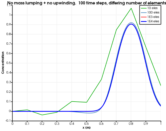
Figure 2: Diffusion as a function of number of elements. The number of time steps is fixed to 100 and no mass lumping and no upwinding is used.
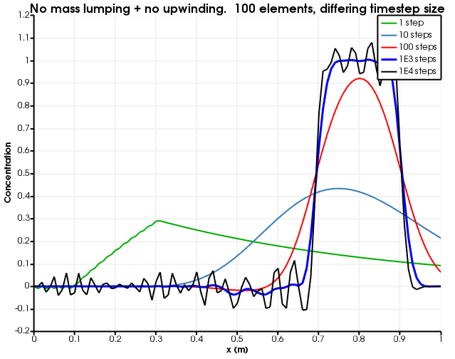
Figure 3: Diffusion as a function of number of time steps. The number of elements is fixed to 100 and no mass lumping and no upwinding is used.
Mass lumping and no upwinding
The MOOSE input file is:
# Using the fully-saturated action, which does mass lumping but no upwinding
[Mesh]
  type = GeneratedMesh
  dim = 1
  nx = 100
  xmin = 0
  xmax = 1
[]

[GlobalParams]
  PorousFlowDictator = dictator
[]

[Variables]
  [./porepressure]
  [../]
  [./tracer]
  [../]
[]

[ICs]
  [./porepressure]
    type = FunctionIC
    variable = porepressure
    function = '1 - x'
  [../]
  [./tracer]
    type = FunctionIC
    variable = tracer
    function = 'if(x<0.1,0,if(x>0.3,0,1))'
  [../]
[]

[PorousFlowFullySaturated]
  porepressure = porepressure
  coupling_type = Hydro
  gravity = '0 0 0'
  fp = the_simple_fluid
  mass_fraction_vars = tracer
[]

[BCs]
  [./constant_injection_porepressure]
    type = DirichletBC
    variable = porepressure
    value = 1
    boundary = left
  [../]
  [./no_tracer_on_left]
    type = DirichletBC
    variable = tracer
    value = 0
    boundary = left
  [../]
  [./remove_component_1]
    type = PorousFlowPiecewiseLinearSink
    variable = porepressure
    boundary = right
    fluid_phase = 0
    pt_vals = '0 1E3'
    multipliers = '0 1E3'
    mass_fraction_component = 1
    use_mobility = true
    flux_function = 1E3
  [../]
  [./remove_component_0]
    type = PorousFlowPiecewiseLinearSink
    variable = tracer
    boundary = right
    fluid_phase = 0
    pt_vals = '0 1E3'
    multipliers = '0 1E3'
    mass_fraction_component = 0
    use_mobility = true
    flux_function = 1E3
  [../]
[]

[Modules]
  [./FluidProperties]
    [./the_simple_fluid]
      type = SimpleFluidProperties
      bulk_modulus = 2E9
      viscosity = 1.0
      density0 = 1000.0
    [../]
  [../]
[]

[Materials]
  [./porosity]
    type = PorousFlowPorosity
    porosity_zero = 0.1
  [../]
  [./permeability]
    type = PorousFlowPermeabilityConst
    permeability = '1E-2 0 0   0 1E-2 0   0 0 1E-2'
  [../]
[]

[Preconditioning]
  active = basic
  [./basic]
    type = SMP
    full = true
    petsc_options = '-ksp_diagonal_scale -ksp_diagonal_scale_fix'
    petsc_options_iname = '-pc_type -sub_pc_type -sub_pc_factor_shift_type -pc_asm_overlap'
    petsc_options_value = ' asm      lu           NONZERO                   2'
  [../]
  [./preferred_but_might_not_be_installed]
    type = SMP
    full = true
    petsc_options_iname = '-pc_type -pc_factor_mat_solver_package'
    petsc_options_value = ' lu       mumps'
  [../]
[]

[VectorPostprocessors]
  [./tracer]
    type = LineValueSampler
    start_point = '0 0 0'
    end_point = '1 0 0'
    num_points = 101
    sort_by = x
    variable = tracer
  [../]
[]

[Executioner]
  type = Transient
  solve_type = Newton
  end_time = 6
  dt = 6E-1
  nl_abs_tol = 1E-8
  timestep_tolerance = 1E-3
[]

[Outputs]
  [./out]
    type = CSV
    execute_on = final
  [../]
[]
Figure 4 and Figure 5 show the dependence on discretisation when there is no upwinding. Evidently, the lack of upwinding causes overshoots and undershoots, and the diffusion becomes less as the spatial discretisation becomes finer.
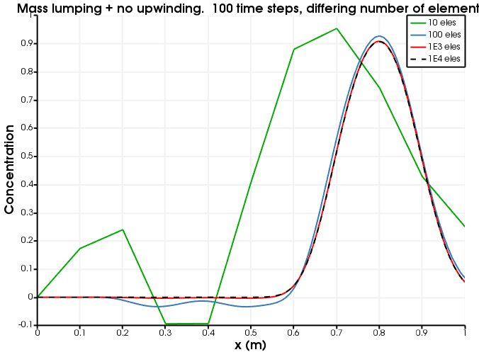
Figure 4: Diffusion as a function of number of elements. The number of time steps is fixed to 100 and no upwinding is used.
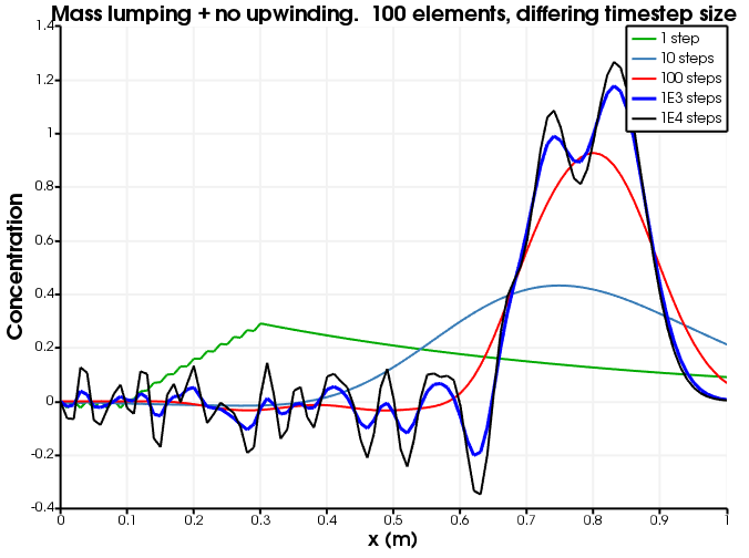
Figure 5: Diffusion as a function of number of time steps. The number of elements is fixed to 100 and no upwinding is used.
Mass lumping and full upwinding
The MOOSE input file is:
# Using upwinded and mass-lumped PorousFlow Kernels
[Mesh]
  type = GeneratedMesh
  dim = 1
  nx = 100
  xmin = 0
  xmax = 1
[]

[GlobalParams]
  PorousFlowDictator = dictator
  gravity = '0 0 0'
[]

[Variables]
  [./porepressure]
  [../]
  [./tracer]
  [../]
[]

[ICs]
  [./porepressure]
    type = FunctionIC
    variable = porepressure
    function = '1 - x'
  [../]
  [./tracer]
    type = FunctionIC
    variable = tracer
    function = 'if(x<0.1,0,if(x>0.3,0,1))'
  [../]
[]

[Kernels]
  [./mass0]
    type = PorousFlowMassTimeDerivative
    fluid_component = 0
    variable = tracer
  [../]
  [./flux0]
    type = PorousFlowAdvectiveFlux
    fluid_component = 0
    variable = tracer
  [../]
  [./mass1]
    type = PorousFlowMassTimeDerivative
    fluid_component = 1
    variable = porepressure
  [../]
  [./flux1]
    type = PorousFlowAdvectiveFlux
    fluid_component = 1
    variable = porepressure
  [../]
[]

[BCs]
  [./constant_injection_porepressure]
    type = DirichletBC
    variable = porepressure
    value = 1
    boundary = left
  [../]
  [./no_tracer_on_left]
    type = DirichletBC
    variable = tracer
    value = 0
    boundary = left
  [../]
  [./remove_component_1]
    type = PorousFlowPiecewiseLinearSink
    variable = porepressure
    boundary = right
    fluid_phase = 0
    pt_vals = '0 1E3'
    multipliers = '0 1E3'
    mass_fraction_component = 1
    use_mobility = true
    flux_function = 1E3
  [../]
  [./remove_component_0]
    type = PorousFlowPiecewiseLinearSink
    variable = tracer
    boundary = right
    fluid_phase = 0
    pt_vals = '0 1E3'
    multipliers = '0 1E3'
    mass_fraction_component = 0
    use_mobility = true
    flux_function = 1E3
  [../]
[]

[Modules]
  [./FluidProperties]
    [./the_simple_fluid]
      type = SimpleFluidProperties
      bulk_modulus = 2E9
      thermal_expansion = 0
      viscosity = 1.0
      density0 = 1000.0
    [../]
  [../]
[]

[UserObjects]
  [./dictator]
    type = PorousFlowDictator
    porous_flow_vars = 'porepressure tracer'
    number_fluid_phases = 1
    number_fluid_components = 2
  [../]
  [./pc]
    type = PorousFlowCapillaryPressureConst
  [../]
[]

[Materials]
  [./temperature]
    type = PorousFlowTemperature
  [../]
  [./ppss]
    type = PorousFlow1PhaseP
    porepressure = porepressure
    capillary_pressure = pc
  [../]
  [./massfrac]
    type = PorousFlowMassFraction
    mass_fraction_vars = tracer
  [../]
  [./simple_fluid]
    type = PorousFlowSingleComponentFluid
    fp = the_simple_fluid
    phase = 0
  [../]
  [./relperm]
    type = PorousFlowRelativePermeabilityConst
    phase = 0
  [../]
  [./porosity]
    type = PorousFlowPorosity
    porosity_zero = 0.1
  [../]
  [./permeability]
    type = PorousFlowPermeabilityConst
    permeability = '1E-2 0 0   0 1E-2 0   0 0 1E-2'
  [../]
[]

[Preconditioning]
  active = basic
  [./basic]
    type = SMP
    full = true
    petsc_options = '-ksp_diagonal_scale -ksp_diagonal_scale_fix'
    petsc_options_iname = '-pc_type -sub_pc_type -sub_pc_factor_shift_type -pc_asm_overlap'
    petsc_options_value = ' asm      lu           NONZERO                   2'
  [../]
  [./preferred_but_might_not_be_installed]
    type = SMP
    full = true
    petsc_options_iname = '-pc_type -pc_factor_mat_solver_package'
    petsc_options_value = ' lu       mumps'
  [../]
[]

[VectorPostprocessors]
  [./tracer]
    type = LineValueSampler
    start_point = '0 0 0'
    end_point = '1 0 0'
    num_points = 101
    sort_by = x
    variable = tracer
  [../]
[]

[Executioner]
  type = Transient
  solve_type = Newton
  end_time = 6
  dt = 6E-1
  nl_abs_tol = 1E-8
  timestep_tolerance = 1E-3
[]

[Outputs]
  [./out]
    type = CSV
    execute_on = final
  [../]
[]
Figure 6 and Figure 7 show the dependence on discretisation when full upwinding is used.
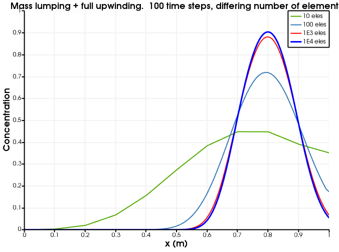
Figure 6: Diffusion as a function of number of elements. The number of time steps is fixed to 100 and full upwinding is used.
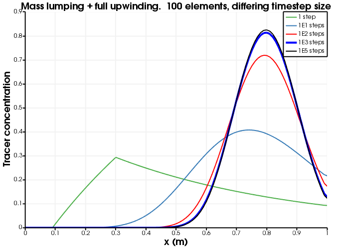
Figure 7: Diffusion as a function of number of time steps. The number of elements is fixed to 100 and full upwinding is used.
RDG(P0)
In RDG, the variables (just the tracer in this case) are constant-monomial, that is, they are constant throughout the element. This means MOOSE behaves like a Finite Volume Method, and it means that the output looks less smooth than the usual linear-Lagrange variables (the figures below display "stepped" results). The MOOSE input file is:
# This test demonstrates the advection of a tracer in 1D using the RDG module.
# There is no slope limiting.  Changing the SlopeLimiting scheme to minmod, mc,
# or superbee means that a linear reconstruction is performed, and the slope
# limited according to the scheme chosen.  Doing this produces RDG(P0P1) and
# substantially reduces numerical diffusion

[Mesh]
  type = GeneratedMesh
  dim = 1
  nx = 100
  xmin = 0
  xmax = 1
[]

[Variables]
  [./tracer]
    order = CONSTANT
    family = MONOMIAL
  [../]
[]

[ICs]
  [./tracer]
    type = FunctionIC
    variable = tracer
    function = 'if(x<0.1,0,if(x>0.3,0,1))'
  [../]
[]

[UserObjects]
  [./lslope]
    type = AEFVSlopeLimitingOneD
    execute_on = 'linear'
    scheme = 'none' #none | minmod | mc | superbee
    u = tracer
  [../]

  [./internal_side_flux]
    type = AEFVUpwindInternalSideFlux
    execute_on = 'linear'
    velocity = 0.1
  [../]

  [./free_outflow_bc]
    type = AEFVFreeOutflowBoundaryFlux
    execute_on = 'linear'
    velocity = 0.1
  [../]
[]

[Kernels]
  [./dot]
    type = TimeDerivative
    variable = tracer
  [../]
[]
[DGKernels]
  [./concentration]
    type = AEFVKernel
    variable = tracer
    component = 'concentration'
    flux = internal_side_flux
    u = tracer
  [../]
[]

[BCs]
  [./concentration]
    type = AEFVBC
    boundary = 'left right'
    variable = tracer
    component = 'concentration'
    flux = free_outflow_bc
    u = tracer
  [../]
[]

[Materials]
  [./aefv]
    type = AEFVMaterial
    slope_limiting = lslope
    u = tracer
  [../]
[]

[VectorPostprocessors]
  [./tracer]
    type = LineValueSampler
    start_point = '0 0 0'
    end_point = '1 0 0'
    num_points = 101
    sort_by = x
    variable = tracer
  [../]
[]

[Executioner]
  type = Transient
  solve_type = PJFNK
  end_time = 6
  dt = 6E-1
  nl_abs_tol = 1E-8
  timestep_tolerance = 1E-3
[]

[Outputs]
  #exodus = true
  csv = true
  execute_on = final
[]
Figure 8 and Figure 9 show the dependence on discretisation when RDG(P0) is used. This is identical to mass-lumping + full-upwinding (up to the fact that constant-monomial variables are used instead of linear-Lagrange). As expected, there are no oscillations or over-shoots or under-shoots, but the results suffer from numerical diffusion.
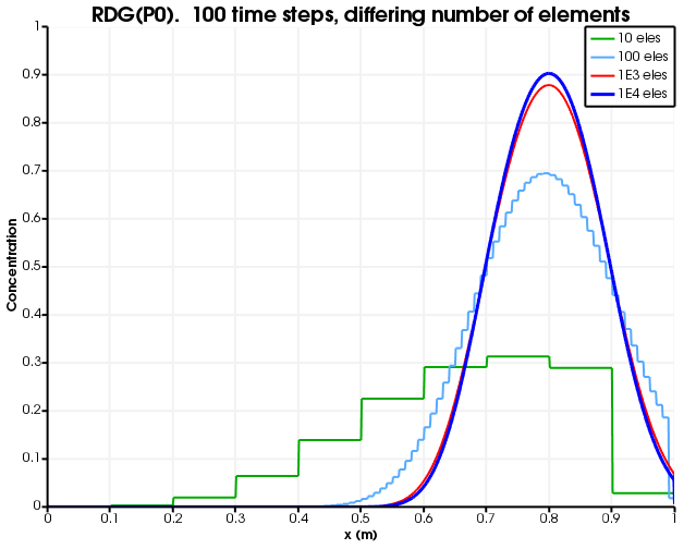
Figure 8: Diffusion as a function of number of elements. The number of time steps is fixed to 100 and RDG(P0) is used.
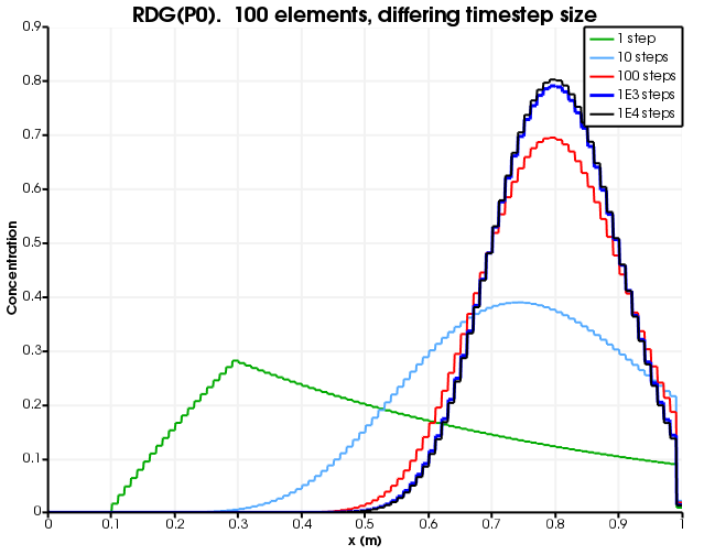
Figure 9: Diffusion as a function of number of time steps. The number of elements is fixed to 100 and RDG(P0) is used.
RDG(P0P1)
The MOOSE input file is almost identical to the RDG(P0) version, save for the changing the SlopeLimiting scheme from "none" to "mc" (or another limiter such as "minmod" or "superbee").
Figure 10 and Figure 11 show the dependence on discretisation when RDG(P0P1) is used. As with RDG(P0), there are no oscillations or over-shoots or under-shoots. However, numerical diffusion is greatly reduced by the linear reconstruction.
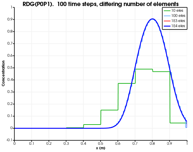
Figure 10: Diffusion as a function of number of elements. The number of time steps is fixed to 100 and RDG(P0P1) is used.
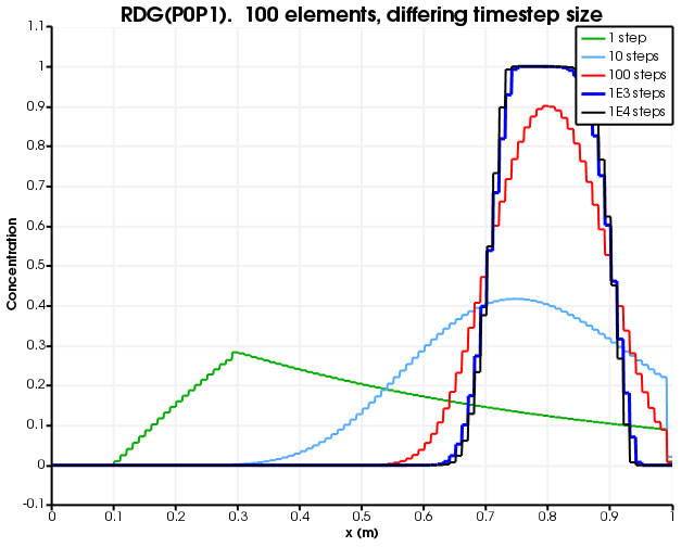
Figure 11: Diffusion as a function of number of time steps. The number of elements is fixed to 100 and RDG(P0P1) is used.
Kuzmin-Turek scheme with no flux limiter
The MOOSE input file is:
# Using Flux-Limited TVD Advection ala Kuzmin and Turek, but without any antidiffusion
[Mesh]
  type = GeneratedMesh
  dim = 1
  nx = 100
  xmin = 0
  xmax = 1
[]

[Variables]
  [./tracer]
  [../]
[]

[ICs]
  [./tracer]
    type = FunctionIC
    variable = tracer
    function = 'if(x<0.1,0,if(x>0.3,0,1))'
  [../]
[]

[Kernels]
  [./mass_dot]
    type = MassLumpedTimeDerivative
    variable = tracer
  [../]
  [./flux]
    type = FluxLimitedTVDAdvection
    variable = tracer
    advective_flux_calculator = fluo
  [../]
[]

[UserObjects]
  [./fluo]
    type = AdvectiveFluxCalculatorConstantVelocity
    flux_limiter_type = none
    u = tracer
    velocity = '0.1 0 0'
  [../]
[]

[BCs]
  [./no_tracer_on_left]
    type = DirichletBC
    variable = tracer
    value = 0
    boundary = left
  [../]
  [./remove_tracer]
# Ideally, an OutflowBC would be used, but that does not exist in the framework
# In 1D VacuumBC is the same as OutflowBC, with the alpha parameter being twice the velocity
    type = VacuumBC
    boundary = right
    alpha = 0.2 # 2 * velocity
    variable = tracer
  [../]
[]

[Preconditioning]
  active = basic
  [./basic]
    type = SMP
    full = true
    petsc_options = '-ksp_diagonal_scale -ksp_diagonal_scale_fix'
    petsc_options_iname = '-pc_type -sub_pc_type -sub_pc_factor_shift_type -pc_asm_overlap'
    petsc_options_value = ' asm      lu           NONZERO                   2'
  [../]
  [./preferred_but_might_not_be_installed]
    type = SMP
    full = true
    petsc_options_iname = '-pc_type -pc_factor_mat_solver_package'
    petsc_options_value = ' lu       mumps'
  [../]
[]

[VectorPostprocessors]
  [./tracer]
    type = LineValueSampler
    start_point = '0 0 0'
    end_point = '1 0 0'
    num_points = 101
    sort_by = x
    variable = tracer
  [../]
[]

[Executioner]
  type = Transient
  solve_type = Newton
  end_time = 6
  dt = 6E-1
  nl_abs_tol = 1E-8
  nl_max_its = 500
  timestep_tolerance = 1E-3
[]

[Outputs]
  [./out]
    type = CSV
    execute_on = final
  [../]
[]
Figure 12 and Figure 13 show the dependence on discretisation when Kuzmin-Turek with no flux limiter is used. As expected, the behaviour is identical to the case with full upwinding.
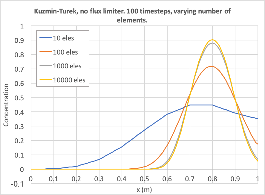
Figure 12: Diffusion as a function of number of elements. The number of time steps is fixed to 100 and Kuzmin-Turek with no flux limiter is used.
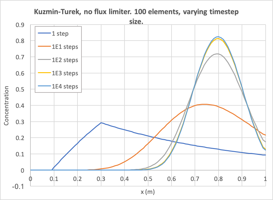
Figure 13: Diffusion as a function of number of time steps. The number of elements is fixed to 100 and Kuzmin-Turek with no flux limiter is used.
Kuzmin-Turek scheme with flux limiter
The MOOSE input file is:
# Using Flux-Limited TVD Advection ala Kuzmin and Turek, with antidiffusion from superbee flux limiting
[Mesh]
  type = GeneratedMesh
  dim = 1
  nx = 100
  xmin = 0
  xmax = 1
[]

[Variables]
  [./tracer]
  [../]
[]

[ICs]
  [./tracer]
    type = FunctionIC
    variable = tracer
    function = 'if(x<0.1,0,if(x>0.3,0,1))'
  [../]
[]

[Kernels]
  [./mass_dot]
    type = MassLumpedTimeDerivative
    variable = tracer
  [../]
  [./flux]
    type = FluxLimitedTVDAdvection
    variable = tracer
    advective_flux_calculator = fluo
  [../]
[]

[UserObjects]
  [./fluo]
    type = AdvectiveFluxCalculatorConstantVelocity
    flux_limiter_type = superbee
    u = tracer
    velocity = '0.1 0 0'
  [../]
[]

[BCs]
  [./no_tracer_on_left]
    type = DirichletBC
    variable = tracer
    value = 0
    boundary = left
  [../]
  [./remove_tracer]
# Ideally, an OutflowBC would be used, but that does not exist in the framework
# In 1D VacuumBC is the same as OutflowBC, with the alpha parameter being twice the velocity
    type = VacuumBC
    boundary = right
    alpha = 0.2 # 2 * velocity
    variable = tracer
  [../]
[]

[Preconditioning]
  active = basic
  [./basic]
    type = SMP
    full = true
    petsc_options = '-ksp_diagonal_scale -ksp_diagonal_scale_fix'
    petsc_options_iname = '-pc_type -sub_pc_type -sub_pc_factor_shift_type -pc_asm_overlap'
    petsc_options_value = ' asm      lu           NONZERO                   2'
  [../]
  [./preferred_but_might_not_be_installed]
    type = SMP
    full = true
    petsc_options_iname = '-pc_type -pc_factor_mat_solver_package'
    petsc_options_value = ' lu       mumps'
  [../]
[]

[VectorPostprocessors]
  [./tracer]
    type = LineValueSampler
    start_point = '0 0 0'
    end_point = '1 0 0'
    num_points = 101
    sort_by = x
    variable = tracer
  [../]
[]

[Executioner]
  type = Transient
  solve_type = Newton
  end_time = 6
  dt = 6E-2
  nl_abs_tol = 1E-8
  nl_max_its = 500
  timestep_tolerance = 1E-3
[]

[Outputs]
  [./out]
    type = CSV
    execute_on = final
  [../]
[]
Figure 14 and Figure 15 show the dependence on discretisation when Kuzmin-Turek with a flux limiter is used (the "superbee" limiter has been chosen in this case, see the worked example of Kuzmin-Turek stabilization). As expected, the behaviour is similar to the RDG(POP1) case, except it is smooth because the variables are linear-lagrange.
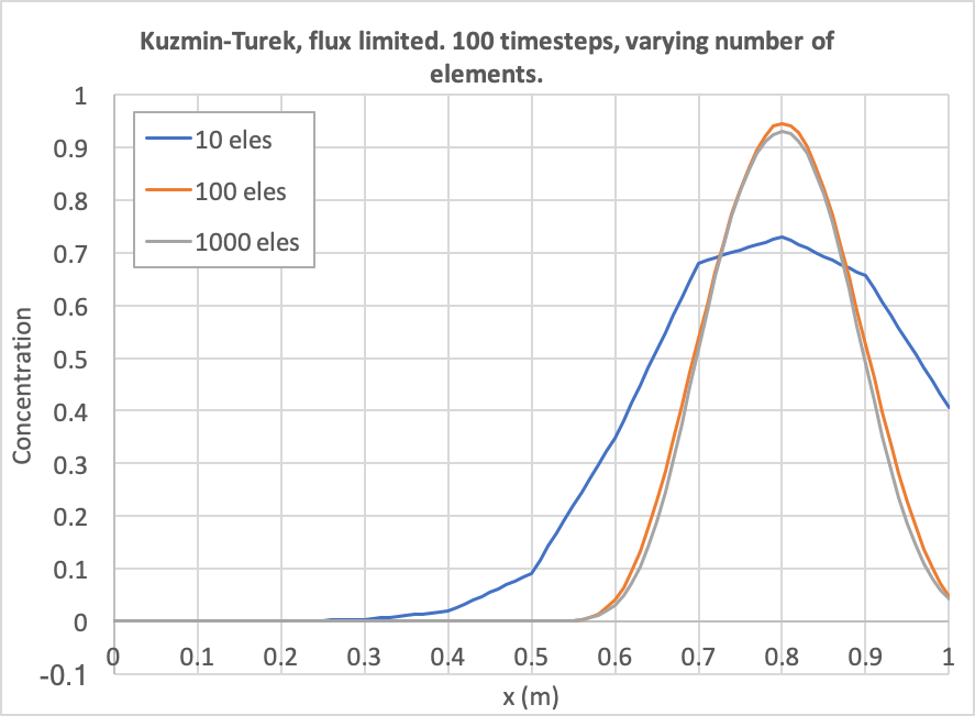
Figure 14: Diffusion as a function of number of elements. The number of time steps is fixed to 100 and Kuzmin-Turek with no flux limiter is used.
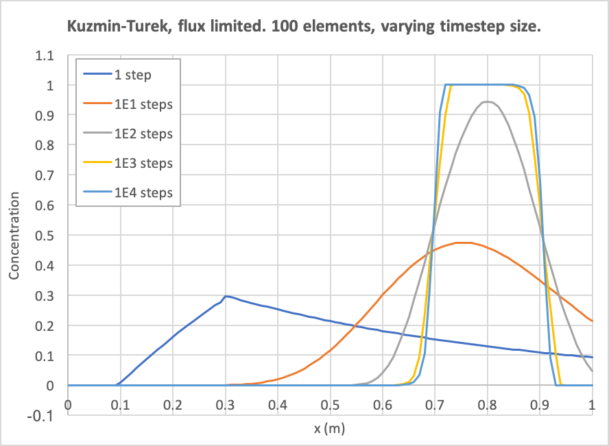
Figure 15: Diffusion as a function of number of time steps. The number of elements is fixed to 100 and Kuzmin-Turek with no flux limiter is used.
Summary
By way of comparison, Figure 16 and Figure 17 show the results when the number of elements is fixed to 100 and the number of timesteps is 100 or 1000 (respectively). Evidently, without upwinding, the result includes over-shoots and under-shoots, which are typically devastating for PorousFlow simulations, since they typically manifest themselves as negative saturations, negative mass fractions, or negative temperatures. With upwinding, RDG(P0), or Kuzmin-Turek with no antidiffusion these are avoided, at the expense of introducing large numerical diffusion. RDG(P0P1) and Kuzmin-Turek with a flux limiter produces a similar amount of numerical diffusion to the non-upwinded, non-masslumped version, but without introducing any over-shoots and under-shoots.
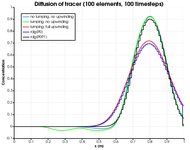
Figure 16: Diffusion for different numerical schemes. 100 timesteps are used.
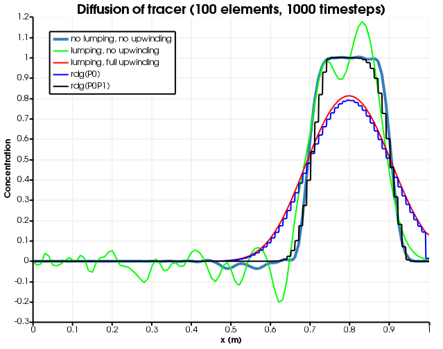
Figure 17: Diffusion for different numerical schemes. 1000 timesteps are used.
Interestingly, as the timestep size is decreased, the numerical diffusion is decreased when using lumping and upwinding, but only up to a point: increasing the number of timesteps from 100 to 10000 makes basically no difference when the number of elements is 100. This suggests that lumping and full-upwinding will always produce numerical diffusion, and this may be proved by simple analysis (not presented here) since the tracer always gets moved from upwind node to downwind node irrespective of the concentration of the tracer.