Inverse Optimization
This page provides a practical overview of the theory and equations needed to solve inverse optimization problems for users/developers of the optimization module. This overview focuses on optimization problems constrained by the solution to a partial differentiation equation, i.e. PDE constrained optimization, and how to efficiently compute the various gradients needed to accelerate the convergence of the optimization solver. See citations throughout this overview for a more in depth and rigorous overview of inverse optimization. This overview on inverse optimization in the optimization module is split up into the following sections:
PDE constrained Optimization Theory: Describes the theory for partial differential equation (PDE) constrained optimization
Adjoint Equation and Boundary Conditions: Derivation of the Adjoint equation using Lagrange multipliers and its boundary conditions.
Parameter Derivatives of PDE: Derivatives of the PDE with respect to the optimization parameters for force and material inversion. Force inversion examples where PDE constrained optimization is used to parameterize boundary conditions and body loads is provided in this section. Material inversion examples are provided in this section where PDE constrained optimization is used to control material properties.
The overall flow of the optimization algorithm implemented in the MOOSE optimization module is shown in Figure 1. In this example, the internal heat source, , is being parameterized to match the simulated and experimental steady state temperature fields, and , respectively. Step one of the optimization cycle consists of adjusting the internal heat source, . In step two, the physics model is solved with the current to obtain a simulated temperature field, . Step two is often referred to as the forward solve. In step three, the simulated and experimental temperature fields are compared via the objective function, . If is below the user defined threshold, the optimization cycle stops and the best fit parameterization of is found. If is above the user defined threshold, the optimization algorithm determines a new and the process is repeated. In the next section, methods for determining the next iteration of the parameterized value, in this case , will be presented. Problems solved using the optimization module are available on the Examples page.
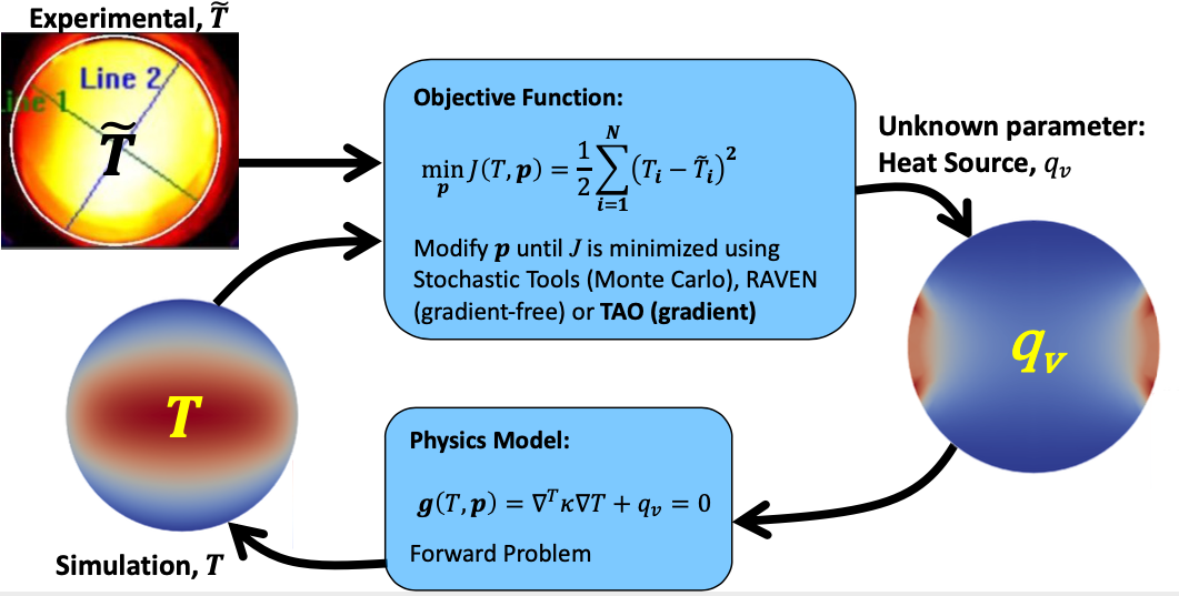
Figure 1: Optimization cycle example for parameterizing an internal heat source distribution to match the simulated and experimental temperature field, and , respectively.
PDE Constrained Inverse Optimization
Inverse optimization is a mathematical framework to infer model parameters by minimizing the misfit between the experimental and simulation observables. In the optimization module, our model is a PDE describing the physics of the experiment. We solve our physics PDE using the finite element method as implemented in MOOSE. The physics of our problem constrains our optimization algorithm. A PDE-constrained inverse optimization framework is formulated as an abstract optimization problem Biegler et al. (2003): (1) where is our objective function which provides a scalar measure of the misfit between experimental and simulated responses, along with any regularization Neumaier (1998). The constraint, , is the residual vector for the PDEs governing the multiphysics phenomena simulated by MOOSE (e.g. coupled heat and elasticity equations), the vector contains design variables (e.g. material properties or loads) and the vector contains state variables (e.g. temperature and displacement fields). Eq. (1) appears simple on the outset but is extremely difficult to solve. The solution space can span millions of degrees of freedom and the parameter space can also be very large. Finally, the PDEs can be highly nonlinear, time-dependent and tightly coupling complex phenomena across multiple physics.
Optimization problems can be solved using either global (gradient-free) or local (gradient-based) approaches Aster et al. (2018). Global approaches require a large number of iterations compared to gradient-based approaches (e.g. conjugate gradient or Newton-type methods), making the latter more suitable to problems with a large parameter space and computationally expensive models. The PETSc TAO optimization library Balay et al. (2019) is used to solve Eq. (1). Optimization libraries like TAO require access to functions for computing the objective (), gradient and Hessian or a function to take the action of the Hessian on a vector. An objective function measuring the misfit or distance between the simulation and experimental data usually has the form (2) where the first summation over is an L norm or euclidean distance between experimental measurement points, , and the simulated solution, . The second summation over provides Tikhonov regularization of the design variables, , for ill-posed problems where controls the amount of regularization. Other types of regularization may also be used.
Gradient-free optimization solvers only require a function to solve for the objective given in Eq. (2). Solving for the objective only requires solving a forward problem to determine and then plugging that into Eq. (2) to determine . The forward problem is defined as the FEM model of the experiment which the analyst should have already made before attempting to perform optimization. The parameters that go into the forward problem (e.g. pressure distributions on sidesets or material properties) are adjusted by the optimization solver and the forward problem is recomputed. This process continues until is below some user defined threshold. The basic gradient-free solver available in TAO is the simplex or Nelder-Mead method. Gradient-free optimization solvers are robust and straight-forward to use. Unfortunately, their computational cost scales exponentially with the number of parameters. When the forward model is a computationally expensive FEM model, gradient-free approaches quickly become computationally expensive.
Gradient-based optimization algorithms require fewer iterations but require functions to solve for the gradient vector and sometimes Hessians matrix. TAO has petsc_options to evaluate finite difference based gradients and Hessians by solving the objective function multiple times with perturbed parameters, which also requires multiple solves of the forward problem. Finite difference gradients and Hessians are good for testing an optimization approach but become too expensive for realistic problems.
Given the large parameter space, we resort to the adjoint method for gradient computation; unlike finite difference approaches, the computational cost of adjoint methods is independent of the number of parameters Plessix (2006). In the adjoint method, the gradient, i.e. the total derivative , is computed as, (3) where accounts for the regularization in Eq. (2) and is the adjoint variable solved for from the adjoint equation (4) where is the adjoint of the Jacobian from the residual vector of the forward problem, , and is a body force like term that accounts for the misfit between the computed and experimental data. Thus, the solution to Eq. (4) has the same complexity as the solution to the forward problem.
The remaining step for evaluating the derivative of the PDE in Eq. (3) is to compute , the derivative of the PDE with respect to the parameter vector. The form this term takes is dependent on the physics (e.g. mechanics or heat conduction) and the parameter being optimized (e.g. force inversion versus material inversion). In what follows, we will derive the adjoint equation for steady state heat conduction and the gradient term for both force and material inversion.
In the following, the adjoint method given in Eq. (3) and Eq. (4) is derived from Eq. (2) following the derivation given by Bradley (2013). Neglecting the regularization in Eq. (2) the total derivative of with respect to using the chain rule is given by (5) We can solve easily compute and so we need to rearrange The physics constraint of the PDE from Eq. (1), , implies that (6) Rearranging the last part of Eq. (6) gives (7) which can be substituted into Eq. (5) to give (8) The terms in Eq. (8) are all terms we can compute. The derivative of the objective with respect to the degree of freedom, , is dependent on the data being fit and will be discussed in the section discussing the adjoint method for discrete data points. The term, , requires differentiation of our PDE with respect to each parameter being inverted for and is derived for simple cases in the following section for force inversion and material identification. The middle term, , is the Jacobian matrix of the forward problem. Eq. (8) requires the inverse of the Jacobian matrix which is not how we actually solve this system of equations.
We have two options for dealing with the inverse of the Jacobian. In the first, we could perform one linear solve per parameter, , being fit by solving . This algorithm scales with the number of parameters which makes it computationally expensive for tens of parameters.
The alternative that we will use is the adjoint method which scales independently to the number of optimization parameters. The adjoint method requires one additional solve of the same complexity as the original forward problem. The adjoint equation given in Eq. (4) is found by setting the adjoint variable, , equal to the first two terms of Eq. (8) and then rearranging terms to give (9) where each step of the derivation has been included as a reminder of how Eq. (4) is obtained. The next section uses an alternative approach to determine the adjoint equation based on Lagrange multipliers Walsh et al. (2013).
Adjoint Problem for Steady State Heat Conduction
In this section, we are interested in solving the following PDE-constrained optimization problem from Eq. (1) for steady state heat conduction: (10) where is the objective function from Eq. (2) without regularization, is the distributed heat flux, is the experimental temperature being compared to our simulation temperature field at discrete locations, . Other forms for the objective function are possible such as different norms or different types of measurements that may require integration over a line or volume.
We also have the following boundary conditions for our PDE, (11) where is the normal vector, is the Dirichlet boundary, and is the Robin or mixed boundary. Common cases for are: (12) where is the heat transfer coefficient and is independent of . The objective function can also be expressed in a integral form for the case of point measurements as follows (13)
We take the equivalent, variational approach to derive the adjoint. Thus, the Lagrangian of this problem is (14) The divergence theorem is applied to the last term in Eq. (14) giving By substituting the above and Eq. (13) into Eq. (14), we have (15) where is the Lagrange multiplier field known as the adjoint state or costate variable. The Lagrangian has been broken up into terms integrated over the body, , and boundary terms, . In order to determine the boundary conditions for the adjoint equation, the boundary integral terms, , in Eq. (15) are further broken up into their separate domains, and , given in Eq. (11) resulting in (16) where is the prescribed temperature on the Dirichlet boundary, . The variation of with respect to is then given by where the variation of the body terms with respect to are given by (17) and the variation of with respect to is given as (18) where for the convection BC given in Eq. (12). Combining Eq. (17) and Eq. (18) to get results in (19)
Stationarity of would require for all admissible . Setting each of the integrals in Eq. (19) results in the adjoint problem and its boundary conditions (20) Solving Eq. (20) comes down to adjusting the boundary conditions and load vector from the forward problem and re-solving.
PDE Derivatives for Inversion
In this section we will present derivatives for steady state heat conduction Eq. (10) with respect to the force or material parameters. For all of these examples, measurement data is taken at specific locations where the objective function can be represented by Eq. (13). We will present the discrete forms of our PDE and its derivative which most closely matches the implementation that will be used in MOOSE.
The discrete form of the PDE constraint for steady state heat conduction in Eq. (10) is given by the residual, , as
(21) where is the Jacobian matrix, and are the discretized temperature and source vectors. Element-wise definitions of the terms are (22) where denotes the continuous Lagrange finite element shape function at node . The solution can be expressed as . Note here the includes the contribution from both the body load term ( in Eq. (10)) and flux boundary conditions (see Eq. (11)). We are assuming a Galerkin form for our discretized PDE by making our test and trial functions identical (both are ). Note in the rest of this document, we omit the superscript of the shape function (i.e., ) and the summation over all the elements (i.e., ) for simplicity.
To compute the derivative of PDE with respect to the design parameters, i.e., , it can be seen from Eq. (22) that the derivatives can come from either or . For problems that have design parameters that are embedded in and/or the Neumann boundary condition in , we call them force inversion problems, since the derivative only depends on the body load. For design parameters that are embedded in and/or the convection boundary condition in , indicating dependence on the material property, we call them material inversion problems. Derivative calculation of different force inversion and material inversion problems are included in the following subsections:
Examples for force and material inversion are given on the following pages:
PDE Derivatives for Force Inversion
We will first consider the simple case of load parameterization for body loads, (in Eq. (10)), where the gradient is given as (23) by taking the chain rule from Eq. (21) and Eq. (22). The gradient term requires the derivative of to be integrated over the volume .
For the first case, we will consider a volumetric heat source that varies linearly across the body, which is given by with and the design parameters. Therefore, the derivative can be calculated as (24) An example using the derivative given in Eq. (24) is given in the Distributed Body Load Example .
In the next force inversion case, we parameterize the intensity of point heat sources, where the heat source takes the form The corresponding gradient term is given by (25) which makes the gradient equal to one at the locations of the point loads. This PDE derivative is used in the Point Loads Example.
Next, we will use force inversion to parameterize a Neumann boundary condition with the heat flux on the boundary being a function of the coordinates, , given by (26) where the derivative of is now integrated over the boundary . For instance, if we have a linearly varying heat flux with and the design parameters, then (27) The derivative given in Eq. (27) is used in the Neumann Boundary Condition Example.
The above force inversion examples, Eq. (23) and Eq. (27), are all linear optimization problems where the parameter being optimized does not show up in the derivative term. Linear optimization problems are not overly sensitive to the location of measurement points or the initial guesses for the parameter being optimized, making them easy to solve. In the following we parameterize a Gaussian body force given by (28) where is the height or intensity of the Gaussian curve, is the location of the peak of the curve, and is the standard deviation of the curve or its width. Parameterizing a Gaussian curve can result in a linear or nonlinear optimization problem depending on which parameter is being optimized. Parameterizing this function for the height, , results in the following linear optimization problem derivative (29) where the parameter being optimized does not show up in the derivative term. However, if we try to parameterize for the location of the peak of the Gaussian curve, , we get the following nonlinear optimization problem derivative (30) where the parameter remains in the derivative term. Optimizing for the peak location of a Gaussian heat source, Eq. (30), will be a much more difficult problem to solve than Eq. (29) and convergence will be dependent on the initial guesses given for and the locations where measurement data is taken.
PDE Derivative for Convective Boundary Conditions
In this section, the convective heat transfer coefficient, , is considered as a parameter for the convection boundary condition given in Eq. (12). This is a material inversion problem with integral limited to the boundary, . The boundary condition is given by on . The PDE derivative term is given by (31) This derivative requires the solution from the forward problem to be included in the integral over the boundary making this a nonlinear optimization problem. This derivative is used in the Convective Boundary Condition Example.
PDE Derivative for Material Inversion
In force inversion and convective heat transfer inversion, the design parameters only exist in the load terms. For force inversion problems, the derivatives of the residual, , with respect to the design parameters only required differentiation of the load functions, not the Jacobian. In this section, we consider material inversion where the design parameters exist in the Jacobian term requiring it to be differentiated. In the below derivatives, we treat the thermal conductivity () as the design parameter by matching experimentally measured temperature data points. The derivative of is taken with respect to . This requires the derivative of in Eq. (21) leading to (32) where was used in the last line. The gradient term given by Eq. (32) is multiplied by the adjoint variable in Eq. (3), giving
(33) where is used in the last line. Computing the integral in Eq. (33) requires an inner product of the gradients of the adjoint and forward variables. This is much simpler to compute in MOOSE than the integral in Eq. (32) which requires the multiplication of nodal variables with elemental shape function gradients. Material inversion is a nonlinear optimization problem since shows up in the derivative, making the derivative dependent on the solution to the forward problem. The derivative given in Eq. (33) is used in this example where the thermal conductivity of a block is found.
This same procedure is used to a temperature dependent thermal conductivity given by where and are the design parameters. The resultant derivative is then (34)
References
- Richard C Aster, Brian Borchers, and Clifford H Thurber.
Parameter estimation and inverse problems.
Elsevier, 2018.[BibTeX]
- Satish Balay, Shrirang Abhyankar, Mark Adams, Jed Brown, Peter Brune, Kris Buschelman, Lisandro Dalcin, Alp Dener, Victor Eijkhout, W Gropp, and others.
PETSc users manual.
2019.[BibTeX]
- Lorenz T Biegler, Omar Ghattas, Matthias Heinkenschloss, and Bart van Bloemen Waanders.
Large-scale PDE-constrained optimization: an introduction, pages 3–13.
Springer, 2003.[BibTeX]
- Andrew M Bradley.
Pde-constrained optimization and the adjoint method.
Technical Report, Technical Report. Stanford University. https://cs. stanford. edu/˜ ambrad …, 2013.[BibTeX]
- Arnold Neumaier.
Solving ill-conditioned and singular linear systems: a tutorial on regularization.
SIAM review, 40(3):636–666, 1998.[BibTeX]
- R-E Plessix.
A review of the adjoint-state method for computing the gradient of a functional with geophysical applications.
Geophysical Journal International, 167(2):495–503, 2006.[BibTeX]
- Timothy Francis Walsh, Wilkins Aquino, and Michael Ross.
Source identification in acoustics and structural mechanics using sierra/sd.
Technical Report, Duke University, Durham, NC; Sandia National Laboratory, Albuquerque, NM …, 2013.[BibTeX]