Force Inversion Example: Point Loads
Background
The MOOSE optimization module provides a flexible framework for solving inverse optimization problems in MOOSE. This page is part of a set of examples for different types of inverse optimization problems.
Example 1: Point Loads
In this example we are parameterizing the heat source intensity at the locations indicated by the symbols in Figure 1 that will produce a temperature field that most closely matches the temperature measurements taken at the points indicated by the symbols. Dirichlet boundary conditions are applied to the entire boundary with T=300.
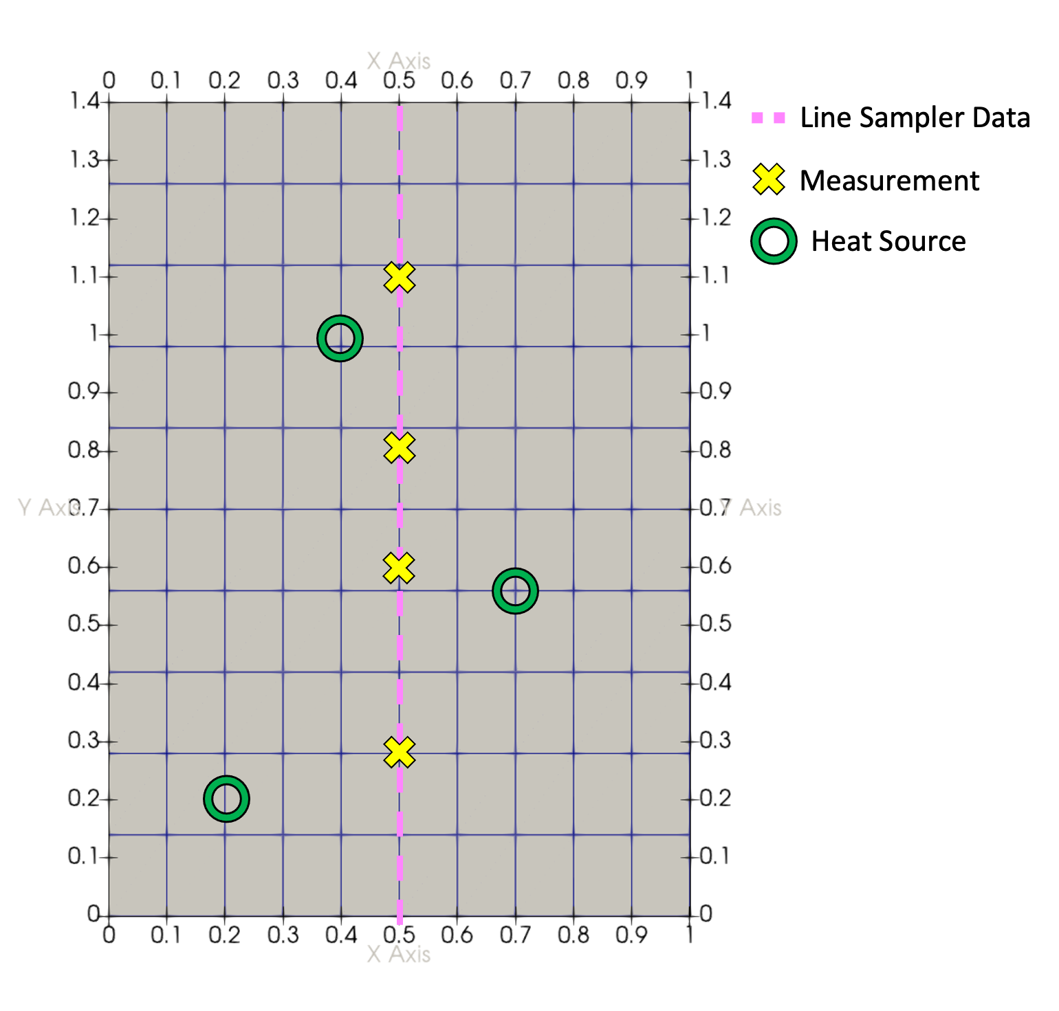
Figure 1: Meshed geometry with measurement () and parameterized point load () locations.
The temperature field with a known heat source is shown in Figure 2. This will be used as synthetic measurement data in the optimization example where the magnitude of the point sources () will be parameterized to best match the temperatures at the measurement locations ().
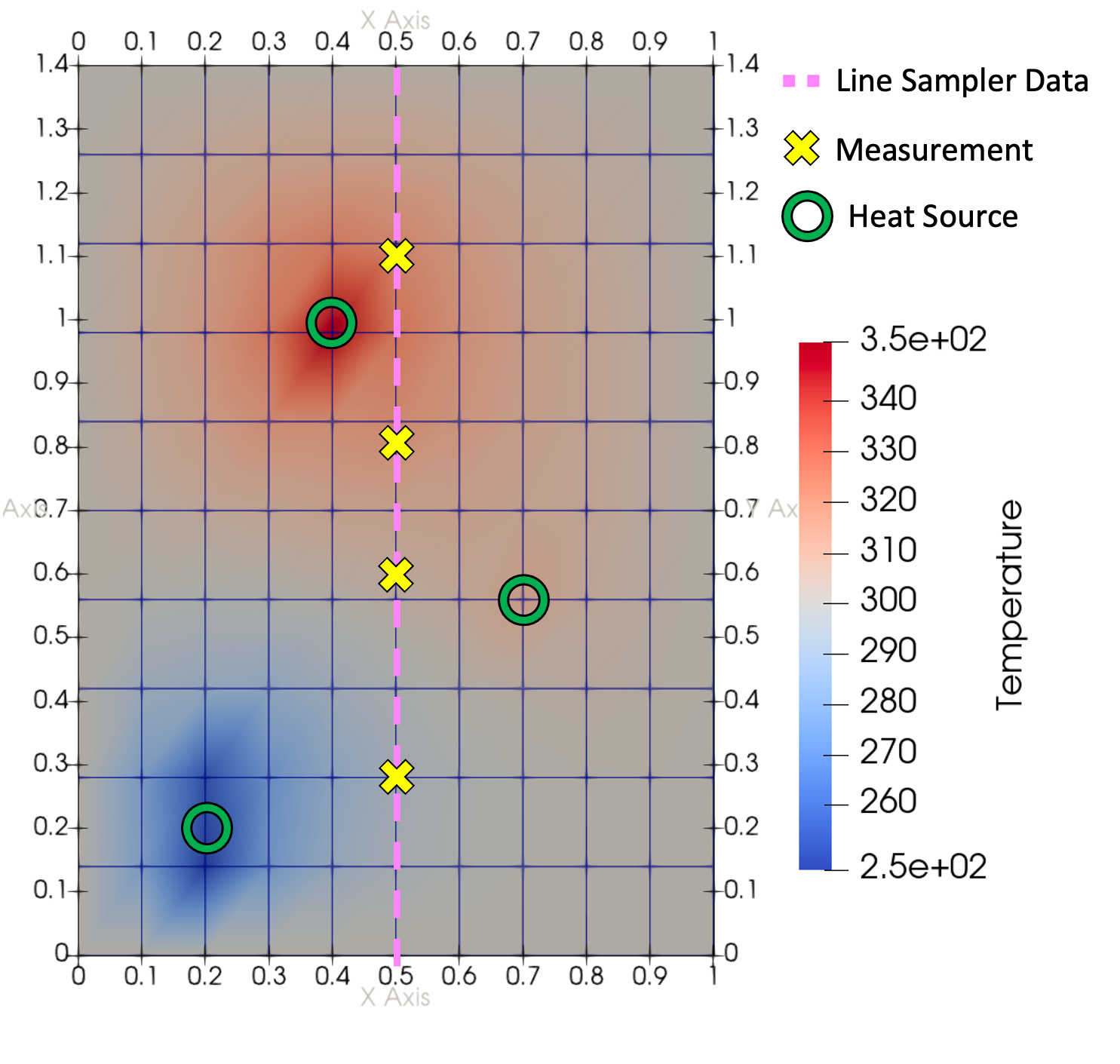
Figure 2: Synthetic temperature field for known heat sources for optimization example.
Main Application Input
Optimization problems are solved using the MultiApps system. The main application contains the optimization executioner and the sub-applications solve the forward and adjoint PDE. The main application input is shown in Listing 1.
Listing 1: Main application optimization input for point load parameterization shown in Figure 1
# DO NOT CHANGE THIS TEST
# this test is documented as an example in forceInv_pointLoads.md
# if this test is changed, the figures will need to be updated.
measurement_points = '0.5 0.28 0
   0.5 0.6 0
   0.5 0.8 0
   0.5 1.1 0'
measurement_values = '293 304 315 320'
[Optimization]
[]

[OptimizationReporter]
  type = GeneralOptimization
  objective_name = objective_value
  parameter_names = 'parameter_results'
  num_values = '3'
[]

[Reporters]
  [main]
    type = OptimizationData
    measurement_points = ${measurement_points}
    measurement_values = ${measurement_values}
  []
[]

[Executioner]
  type = Optimize
  tao_solver = taonls
  petsc_options_iname = '-tao_gttol -tao_max_it -tao_nls_pc_type -tao_nls_ksp_type'
  petsc_options_value = '1e-5 10 none cg'
  verbose = true
[]

[MultiApps]
  [forward]
    type = FullSolveMultiApp
    input_files = forward.i
    execute_on = "FORWARD"
  []
  [adjoint]
    type = FullSolveMultiApp
    input_files = adjoint.i
    execute_on = "ADJOINT"
  []
  [homogeneousForward]
    type = FullSolveMultiApp
    input_files = forward_homogeneous.i
    execute_on = "HOMOGENEOUS_FORWARD"
  []
[]

[Transfers]
  # FORWARD transfers
  [toForward_measument]
    type = MultiAppReporterTransfer
    to_multi_app = forward
    from_reporters = 'main/measurement_xcoord
                      main/measurement_ycoord
                      main/measurement_zcoord
                      main/measurement_time
                      main/measurement_values
                      OptimizationReporter/parameter_results'
    to_reporters = 'measure_data/measurement_xcoord
                    measure_data/measurement_ycoord
                    measure_data/measurement_zcoord
                    measure_data/measurement_time
                    measure_data/measurement_values
                    point_source/value'
  []
  [fromForward]
    type = MultiAppReporterTransfer
    from_multi_app = forward
    # Note: We are transferring the misfit values into main misfit
    from_reporters = 'measure_data/objective_value measure_data/misfit_values'
    to_reporters = 'OptimizationReporter/objective_value main/misfit_values'
  []

  # ADJOINT transfers
  #NOTE:  the adjoint variable we are transferring is actually the gradient
  [toAdjoint]
    type = MultiAppReporterTransfer
    to_multi_app = adjoint
    from_reporters = 'main/measurement_xcoord
                      main/measurement_ycoord
                      main/measurement_zcoord
                      main/measurement_time
                      main/misfit_values'
    to_reporters = 'misfit/measurement_xcoord
                    misfit/measurement_ycoord
                    misfit/measurement_zcoord
                    misfit/measurement_time
                    misfit/misfit_values'
  []
  [fromAdjoint]
    type = MultiAppReporterTransfer
    from_multi_app = adjoint
    from_reporters = 'gradient/adjoint'
    to_reporters = 'OptimizationReporter/grad_parameter_results'
  []

  # HESSIAN transfers.  Same as forward.
  [toHomoForward]
    type = MultiAppReporterTransfer
    multi_app = homogeneousForward
    direction = to_multiapp
    from_reporters = 'main/measurement_xcoord
                      main/measurement_ycoord
                      main/measurement_zcoord
                      main/measurement_time
                      main/measurement_values
                      OptimizationReporter/parameter_results'
    to_reporters = 'measure_data/measurement_xcoord
                    measure_data/measurement_ycoord
                    measure_data/measurement_zcoord
                    measure_data/measurement_time
                    measure_data/measurement_values
                    point_source/value'
  []
  [fromHomoForward]
    type = MultiAppReporterTransfer
    multi_app = homogeneousForward
    direction = from_multiapp
    # Note: We are transferring the simulation values into misfit
    # this has to be done when using general opt and homogenous forward.
    from_reporters = 'measure_data/simulation_values'
    to_reporters = 'main/misfit_values'
  []
[]

[Reporters]
  [optInfo]
    type = OptimizationInfo
  []
[]

[Outputs]
  csv = true
[]
The main application runs the optimization executioner and transfers data from the optimization executioner back and forth to the sub-apps that are running the "forward" and "adjoint" simulations.
Since no mesh or physics kernels are required on the main-app, we use the Optimization action to set up all of the nullkernels, empty mesh, etc. needed to get a MOOSE simulation to run.
The Optimize executioner block in Listing 2 , provides an interface with the PETSc TAO optimization library. The optimization algorithm is selected with "tao_solver" with specific solver options set with petsc_options. In this example the TAO Hessian based Newton linesearch algorithm is selected with taonls.
Listing 2: Main application Executioner block for point load parameterization shown in Figure 1
[Executioner]
  type = Optimize
  tao_solver = taonls
  petsc_options_iname = '-tao_gttol -tao_max_it -tao_nls_pc_type -tao_nls_ksp_type'
  petsc_options_value = '1e-5 10 none cg'
  verbose = true
[]
The optimize executioner requires an OptimizationReporter. In this example the GeneralOptimization reporter is used. A GeneralOptimization reporter is used to transfer data between the optimization executioner and the transfers used for communicating with the sub-apps. The "objective_name" is used to name the reporter that holds the objective value to optimize. "parameter_names" are the list of parameters being controlled. A gradient reporter is automatically created for each parameter with a name that is "grad_" concatenated to the parmater name provided. The "num_values" specifies the number of parameters per group of parameter_names being controlled. In this case there is a single parameter being controlled and that parameter contains three values being controlled. These three values are the magnitude of the point loads being applied, shown by the symbols in Figure 1. "initial_condition" can be used to supply initial guesses for parameter values. Bounded optimization algorithms like bounded conjugate gradient (taobncg) will use the bounds supplied by "lower_bounds" and "upper_bounds". Unbounded solvers like taonls used in this example will not apply the bounds even if they are in the input file.
The "measurement_points" are the xyz coordinates of the measurement data and "measurement_values" are the values at each measurement point. For this small example, the measurement data are supplied in the input file but for larger sets of measurement data, there is the option to read these values from a csv file using "measurement_file" and "file_value".
Listing 3: Main application OptimizationReporter and Reporter block for point load parameterization shown in Figure 1
[OptimizationReporter]
  type = GeneralOptimization
  objective_name = objective_value
  parameter_names = 'parameter_results'
  num_values = '3'
[]
[Reporters]
  [main]
    type = OptimizationData
    measurement_points = ${measurement_points}
    measurement_values = ${measurement_values}
  []
[]
The MultiApps block is shown in Listing 4. The optimization executioner utilizes FullSolveMultiApp sub-apps which, when the module is linked in, have special "execute_on" flags to allow the optimization executioner to control which sub-app is being solved. This allows TAO to call whichever sub-app it needs in order to compute the quantity needed. For instance, if TAO needs to recompute the objective function with a new set of parameters, it will execute the sub-app with the flag exectute_on=FORWARD. The sub-apps being set-up correspond to the type of optimization algorithm being used. Gradient free algorithms like Nelder-Mead (taonm) only require a forward sub-app. Gradient based optimization algorithms like conjugate gradient (taobncg) require a forward and adjoint sub-app. Hessian based optimization algorithms like Newton linesearch (taonls) requires a forward, adjoint and homogeneous forward sub-app.
Listing 4: Main application MultiApps block for point load parameterization shown in Figure 1
[MultiApps]
  [forward]
    type = FullSolveMultiApp
    input_files = forward.i
    execute_on = "FORWARD"
  []
  [adjoint]
    type = FullSolveMultiApp
    input_files = adjoint.i
    execute_on = "ADJOINT"
  []
  [homogeneousForward]
    type = FullSolveMultiApp
    input_files = forward_homogeneous.i
    execute_on = "HOMOGENEOUS_FORWARD"
  []
[]
Transfers makes up the next section of the main input file. TAO interacts with the various sub-apps using the reporter system and the MultiAppReporterTransfer. The first two Transfers in Listing 5 communicate data with the forward sub-app. These Transfers are used by TAO to compute the objective. The first transfer [toForward_measument] communicates the measurement locations to the forward app object OptimizationData. This transfer can be avoided by placing the OptimizationData block on the forward solve input file instead of the main optimization input file. These are the locations where the objective function is computed by minimizing the difference between the simulated and experimental data at discrete points, see Inverse Optimization, Eq. (13). The second transfer [toForward] is used by TAO to control the parameter being optimized. In this case, [toForward] controls the 'value' reporter in a ConstantVectorPostprocessor on the forward-app which is then consumed by the ReporterPointSource dirac kernel to apply the point source loading. The third transfer, [fromForward] returns the simulation values at the measurement points from the forward-app to the main-app main Reporter which computes a new objective function for TAO.
Listing 5: Main application Transfers for point load parameterization shown in Figure 1
[Transfers]
  # FORWARD transfers
  [toForward_measument]
    type = MultiAppReporterTransfer
    to_multi_app = forward
    from_reporters = 'main/measurement_xcoord
                      main/measurement_ycoord
                      main/measurement_zcoord
                      main/measurement_time
                      main/measurement_values
                      OptimizationReporter/parameter_results'
    to_reporters = 'measure_data/measurement_xcoord
                    measure_data/measurement_ycoord
                    measure_data/measurement_zcoord
                    measure_data/measurement_time
                    measure_data/measurement_values
                    point_source/value'
  []
  [fromForward]
    type = MultiAppReporterTransfer
    from_multi_app = forward
    # Note: We are transferring the misfit values into main misfit
    from_reporters = 'measure_data/objective_value measure_data/misfit_values'
    to_reporters = 'OptimizationReporter/objective_value main/misfit_values'
  []

  # ADJOINT transfers
  #NOTE:  the adjoint variable we are transferring is actually the gradient
  [toAdjoint]
    type = MultiAppReporterTransfer
    to_multi_app = adjoint
    from_reporters = 'main/measurement_xcoord
                      main/measurement_ycoord
                      main/measurement_zcoord
                      main/measurement_time
                      main/misfit_values'
    to_reporters = 'misfit/measurement_xcoord
                    misfit/measurement_ycoord
                    misfit/measurement_zcoord
                    misfit/measurement_time
                    misfit/misfit_values'
  []
  [fromAdjoint]
    type = MultiAppReporterTransfer
    from_multi_app = adjoint
    from_reporters = 'gradient/adjoint'
    to_reporters = 'OptimizationReporter/grad_parameter_results'
  []

  # HESSIAN transfers.  Same as forward.
  [toHomoForward]
    type = MultiAppReporterTransfer
    multi_app = homogeneousForward
    direction = to_multiapp
    from_reporters = 'main/measurement_xcoord
                      main/measurement_ycoord
                      main/measurement_zcoord
                      main/measurement_time
                      main/measurement_values
                      OptimizationReporter/parameter_results'
    to_reporters = 'measure_data/measurement_xcoord
                    measure_data/measurement_ycoord
                    measure_data/measurement_zcoord
                    measure_data/measurement_time
                    measure_data/measurement_values
                    point_source/value'
  []
  [fromHomoForward]
    type = MultiAppReporterTransfer
    multi_app = homogeneousForward
    direction = from_multiapp
    # Note: We are transferring the simulation values into misfit
    # this has to be done when using general opt and homogenous forward.
    from_reporters = 'measure_data/simulation_values'
    to_reporters = 'main/misfit_values'
  []
[]
The next set of Transfers in Listing 5 communicate reporter values between the main-app and adjoint sub-app to compute the gradient of the objective function with respect to the controllable parameter. The third transfer named [toAdjoint] sends the misfit data at each measurement point to an OptimizationData reporter on the adjoint-app which is then consumed by the ReporterPointSource dirackernel to apply the misfit source loading as described by the top equation in Inverse Optimization, Eq. (20). The fourth transfer named [fromAdjoint] retrieves the gradient from the adjoint-app for TAO. The sibling transfer system could have been used to transfer the misfit data directly from the forward solve to the adjoint solve.
The final set of Transfers in Listing 5 communicate reporter values between the main-app and the homogeneous forward sub-app to compute a matrix free Hessian. The homogeneous forward transfers, [toHomoForward_measument] [toHomoForward] and [fromHomoForward] transfer the same reporter data to the same objects types used by the forward-app. For force inversion, the homogeneous forward app solves the same kernels as the forward-app except the boundary conditions are homogenized, i.e. set to zero. The parameter being controlled in OptimizationReporter by the Optimize executioner for the homogeneous forward problem is the variation in the parameter which is determined by TAO in order to build up the required matrix free Hessian. In the Transfer from the homogenous forward sub-app Listing 6, the simulation_values are transferred into the misfit_values in the main application. This will be problem specific to the tpy eof optimization performed.
Listing 6: Main application Transfers block for homogenous forward sub-app shown in Figure 1
[Transfers]
  [fromHomoForward]
    type = MultiAppReporterTransfer
    multi_app = homogeneousForward
    direction = from_multiapp
    # Note: We are transferring the simulation values into misfit
    # this has to be done when using general opt and homogenous forward.
    from_reporters = 'measure_data/simulation_values'
    to_reporters = 'main/misfit_values'
  []
[]
Iteration history of the optimization solve is output by the OptimizationInfo reporter as shown in Listing 7. This reporter tracks the objective function value, norm of the gradient, total number of sub-app evaluations, and the number of forward, adjoint, or Hessian iterations per optimization step.
Listing 7: Main application OptimizationInfo for outputting convergence information.
[Reporters]
  [optInfo]
    type = OptimizationInfo
  []
[]
Forward Sub-Application Input
The forward problem sub-app input file for the point load simulation shown in Figure 1 is given in Listing 8. Tao uses the solution of the forward-app to compute the objective function. Almost every object included in the forward-app input would be needed in a regular simulation of this system with point loads of a known magnitude. The point loads are applied by the ReporterPointSource Dirac kernel. The xyz coordinates and point load value used in the ReporterPointSource come from the reporters defined in the ConstantVectorPostprocessor vector postprocessor. The reporters in the ConstantVectorPostprocessor are over-written by the [toForward] transfer on the main-app each time Tao executes the forward-app. The values being transferred into the ConstantVectorPostprocessor are the values being optimized and are controlled by Tao.
Listing 8: Complete input file for executing the forward problem sub-app.
# DO NOT CHANGE THIS TEST
# this test is documented as an example in forceInv_pointLoads.md
# if this test is changed, the figures will need to be updated.
[Mesh]
  [gmg]
    type = GeneratedMeshGenerator
    dim = 2
    nx = 10
    ny = 10
    xmax = 1
    ymax = 1.4
  []
[]

[Variables]
  [temperature]
  []
[]

[Kernels]
  [heat_conduction]
    type = MatDiffusion
    variable = temperature
    diffusivity = thermal_conductivity
  []
[]

[DiracKernels]
  [pt]
    type = ReporterPointSource
    variable = temperature
    x_coord_name = 'point_source/x'
    y_coord_name = 'point_source/y'
    z_coord_name = 'point_source/z'
    value_name = 'point_source/value'
  []
[]

[BCs]
  [left]
    type = DirichletBC
    variable = temperature
    boundary = left
    value = 300
  []
  [right]
    type = DirichletBC
    variable = temperature
    boundary = right
    value = 300
  []
  [bottom]
    type = DirichletBC
    variable = temperature
    boundary = bottom
    value = 300
  []
  [top]
    type = DirichletBC
    variable = temperature
    boundary = top
    value = 300
  []
[]

[Materials]
  [steel]
    type = GenericConstantMaterial
    prop_names = thermal_conductivity
    prop_values = 5
  []
[]

[Executioner]
  type = Steady
  solve_type = NEWTON
  nl_abs_tol = 1e-6
  nl_rel_tol = 1e-8
  petsc_options_iname = '-pc_type'
  petsc_options_value = 'lu'
[]

[VectorPostprocessors]
  [point_source]
    type = ConstantVectorPostprocessor
    vector_names = 'x y z value'
    value = '0.2 0.7 0.4;
             0.2 0.56 1;
             0 0 0;
             -1000 120 500'
    execute_on = LINEAR
  []
  [vertical]
    type = LineValueSampler
    variable = 'temperature'
    start_point = '0.5 0 0'
    end_point = '0.5 1.4 0'
    num_points = 21
    sort_by = y
  []
[]

[Reporters]
  [measure_data]
    type = OptimizationData
    objective_name = objective_value
    variable = temperature
  []
[]

[Outputs]
  console = false
  file_base = 'forward'
[]
The locations where the simulation values are compared to the measurement data is transferred from the main-app [toForward_measurement] transfer into the forward-app OptimizationData reporter. By specifying the "variable", the reporter will evaluate the simulated temperature at the measurement locations. The main-app [fromForward] transfer then gets the temperature values sampled by OptimizationData back to Tao and the objective function can then be computed.
Adjoint Sub-Application Input
The adjoint problem sub-app computes the adjoint solution of the forward problem for a point load applied at the measurement locations. The adjoint sub-app input file is given in Listing 9. The adjoint variable is used to compute the gradient needed by TAO. The magnitude of the point loads for the adjoint problem are the misfit given by the difference of the measurement and simulation data, as shown by Inverse Optimization, Eq. (20). The misfit is computed by the OptimizationReporter on the main-app and is transferred into the adjoint-app [OptimizationData] object using the main-app [toAdjoint] transfer. The ReporterPointSource consumes the OptimizationData and applies the point loads at the measurement points.
Listing 9: Complete input file for executing the adjoint problem sub-app.
# DO NOT CHANGE THIS TEST
# this test is documented as an example in forceInv_pointLoads.md
# if this test is changed, the figures will need to be updated.
[Mesh]
  type = GeneratedMesh
  dim = 2
  nx = 10
  ny = 10
  xmax = 1
  ymax = 1.4
[]

[Variables]
  [adjoint]
  []
[]

[Problem]
  extra_tag_vectors = 'ref'
[]
[AuxVariables]
  [residual_src]
  []
[]
[AuxKernels]
  [residual_src]
    type = TagVectorAux
    vector_tag = 'ref'
    v = 'adjoint'
    variable = 'residual_src'
  []
[]

[Variables]
  [adjoint]
  []
[]

[Kernels]
  [heat_conduction]
    type = MatDiffusion
    variable = adjoint
    diffusivity = thermal_conductivity
  []
[]

#-----every adjoint problem should have these two
[DiracKernels]
  [pt]
    type = ReporterPointSource
    variable = adjoint
    x_coord_name = misfit/measurement_xcoord
    y_coord_name = misfit/measurement_ycoord
    z_coord_name = misfit/measurement_zcoord
    value_name = misfit/misfit_values
    extra_vector_tags = 'ref'
  []
[]

[Reporters]
  [misfit]
    type = OptimizationData
  []
[]

[BCs]
  [left]
    type = DirichletBC
    variable = adjoint
    boundary = left
    value = 0
  []
  [right]
    type = DirichletBC
    variable = adjoint
    boundary = right
    value = 0
  []
  [bottom]
    type = DirichletBC
    variable = adjoint
    boundary = bottom
    value = 0
  []
  [top]
    type = DirichletBC
    variable = adjoint
    boundary = top
    value = 0
  []
[]

[Materials]
  [steel]
    type = GenericConstantMaterial
    prop_names = thermal_conductivity
    prop_values = 5
  []
[]

[Executioner]
  type = Steady
  solve_type = NEWTON
  nl_abs_tol = 1e-6
  nl_rel_tol = 1e-8
  petsc_options_iname = '-pc_type'
  petsc_options_value = 'lu'
[]

[VectorPostprocessors]
  [gradient]
    type = PointValueSampler
    points = '0.2 0.2 0
              0.7 0.56 0
              0.4 1 0'
    variable = adjoint
    sort_by = id
  []
[]

[Outputs]
  console = false
  exodus = false
  file_base = 'adjoint'
[]
The misfit load applied at the first iteration step is given by the residual values shown in Figure 3. Homogeneous boundary conditions are applied in the adjoint problem. The solution to the adjoint problem for the first iteration is shown in Figure 4. The adjoint variable can be interpreted as the sensitivity of point load locations on the measurement values. Ideally, measurements would be taken at locations that are most sensitive to the point source locations, i.e. the measurement locations maximize the adjoint variable at the point sources.
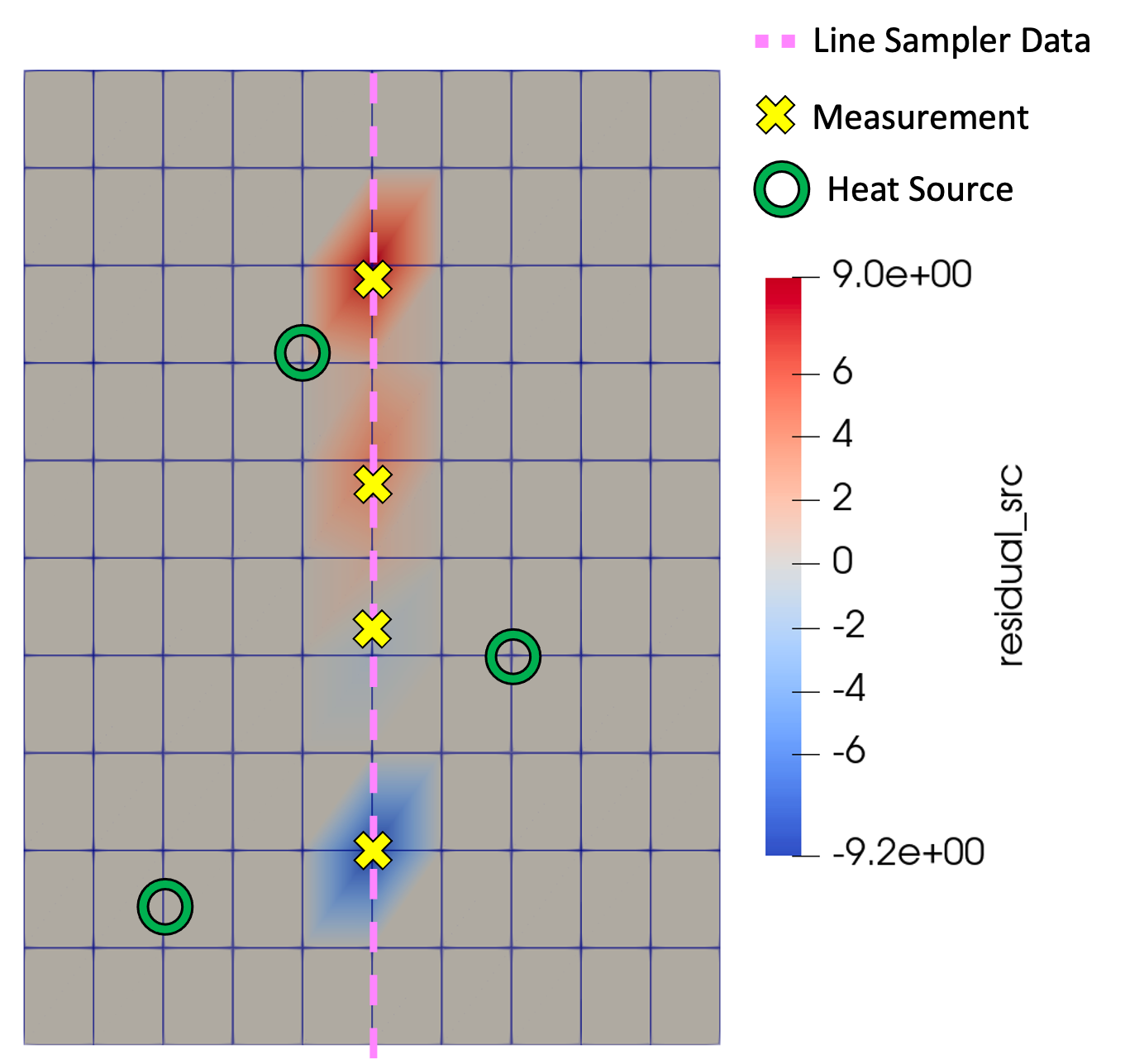
Figure 3: Adjoint misfit load from the first optimization iteration.
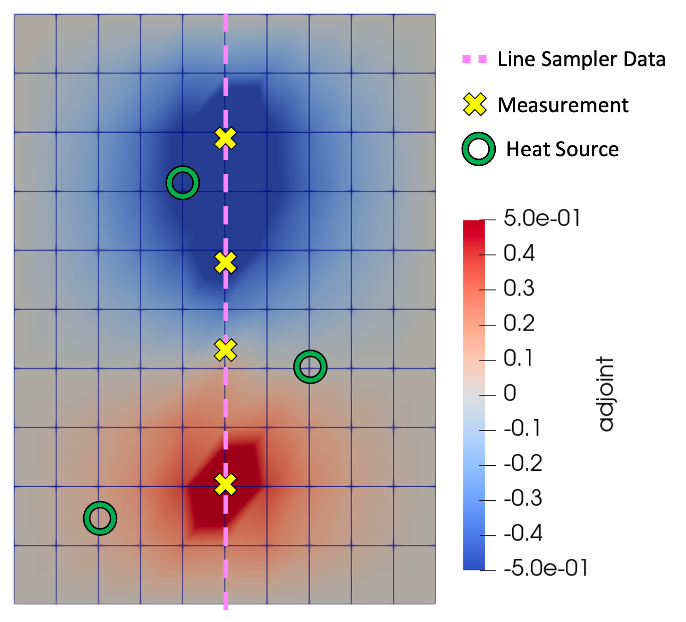
Figure 4: Adjoint solution from the misfit load applied in Figure 3 for the first optimization iteration.
The purpose of the adjoint sub-app is to compute gradient needed by TAO. This gradient is given by
where is the objective function, , is the controllable parameter, is the adjoint variable computed by the adjoint sub-app and is the residual from the forward problem. This gradient ignores regularization shown in Inverse Optimization, Eq. (2) which isn't needed for force inversion problems. For the simple case of point loading, the derivative of the forward problem residual with respect to the parameter, , given by Inverse Optimization, Eq. (25) is a projection matrix equal to 1 at locations where measurements are taken and zero everywhere else. The gradient given by is the adjoint variable sampled at the locations of the point loads. This sampling is done by the PointValueSampler vector postprocessor. The PointValueSampler is then transferred back to main-app in the fromAdjoint transfer and is the gradient used by TAO.
Homogeneous Forward Sub-Application Input
Hessian based optimization algorithms like Newton linesearch (taonls) require a homogeneous version of the forward problem given by the input file Listing 10. A homogenous forward problem is the forward problem with homogenous boundary conditions, i.e. the value or the flux is to zero. A homogenous forward problem is required for Hessian based optimization if a homogenous forward problem cannot be derived, then a gradient based algorithm like conjugate gradient (taobncg) should be used. The forward and homogeneous forward sub-apps have the same parameters transferred to them from the main-app. The parameters transferred into the homogeneous forward problem ConstantVectorPostprocessor vector postprocessor from the main-app [toHomoForward] transfer are perturbations of the parameters computed by TAO. The solution to the homogeneous forward problem is then sampled at the measurement points by OptimizationData and is returned to TAO on the main-app with the [fromHomoForward] transfer to be used as a matrix free Hessian. The matrix free Hessian algorithm is only valid for force inversion and does not work for material inversion. For linear optimization problems, Hessian based optimization algorithms are able to converge on the exact answer in a single iteration.
Listing 10: Complete input file for executing the homogeneous forward problem sub-app.
# DO NOT CHANGE THIS TEST
# this test is documented as an example in forceInv_pointLoads.md
# if this test is changed, the figures will need to be updated.
[Mesh]
  [gmg]
    type = GeneratedMeshGenerator
    dim = 2
    nx = 10
    ny = 10
    xmax = 1
    ymax = 1.4
  []
[]

[Variables]
  [temperature]
  []
[]

[Kernels]
  [heat_conduction]
    type = MatDiffusion
    variable = temperature
    diffusivity = thermal_conductivity
  []
[]

[DiracKernels]
  [pt]
    type = ReporterPointSource
    variable = temperature
    x_coord_name = 'point_source/x'
    y_coord_name = 'point_source/y'
    z_coord_name = 'point_source/z'
    value_name = 'point_source/value'
  []
[]

[BCs]
  [left]
    type = DirichletBC
    variable = temperature
    boundary = left
    value = 0
  []
  [right]
    type = DirichletBC
    variable = temperature
    boundary = right
    value = 0
  []
  [bottom]
    type = DirichletBC
    variable = temperature
    boundary = bottom
    value = 0
  []
  [top]
    type = DirichletBC
    variable = temperature
    boundary = top
    value = 0
  []
[]

[Materials]
  [steel]
    type = GenericConstantMaterial
    prop_names = thermal_conductivity
    prop_values = 5
  []
[]

[Executioner]
  type = Steady
  solve_type = NEWTON
  nl_abs_tol = 1e-6
  nl_rel_tol = 1e-8
  petsc_options_iname = '-pc_type'
  petsc_options_value = 'lu'
[]

[VectorPostprocessors]
  [point_source]
    type = ConstantVectorPostprocessor
    vector_names = 'x y z value'
    value = '0.2 0.7 0.4;
             0.2 0.56 1;
             0 0 0;
             -1000 120 500'
    execute_on = LINEAR
  []
[]

[Reporters]
  [measure_data]
    type = OptimizationData
    variable = temperature
  []
[]

[Outputs]
  console = false
  file_base = 'forward_homo'
[]
Optimization Results
The results for this example are shown in Figure 5. The left plot in Figure 5 shows the temperature along a vertical line passing through the measurement points is taken at several conjugate gradient iterations. The right plot shows the convergence of the objective function for several optimization algorithms. It's important to note when looking at the convergence plot that the Nelder Mead gradient free algorithm requires only a single forward solve per iteration where as the gradient based algorithms require at least two solves, one for the forward problem and one for the adjoint problem. The Hessian based algorithms require several forward, adjoint, and homogenous forward solves per iteration to make the matrix free Hessian accurate enough to converge. Even with this in mind, the Hessian based algorithm is the most computationally efficient for this problem. The taolmvm gradient based method also performs well and only requires an adjoint.
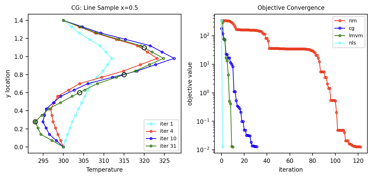
Figure 5: (Left) Temperature field taken along pink dashed line in Figure 1 at conjugate gradient iterations. (Right) Convergence of the objective function for different optimization algorithms.