Numerical diffusion
This page is part of a set of pages devoted to discussions of numerical stabilization in PorousFlow. See:
Numerical diffusion is the artificial smoothing of quantities, such as temperature and concentrations, as they are transported through a numerical model. In the case of PorousFlow, it is usually the fluid that transports these quantities (the fluid "advects" temperature and chemical species). Numerical diffusion can be the major source of inaccurate results in simulations, as MOOSE predicts that tracer breakthrough times (etc) are much shorter than they are in reality.
An animation of the tracer advection is shown in Figure 1. Notice that the initially-sharp profile suffers from diffusion.
Figure 1: Tracer advection down the porepressure gradient.
Numerical diffusion has been mentioned in various pieces of PorousFlow documentation (eg, in the Porous Flow Tutorial Page 06. Adding a tracer and PorousFlowFullySaturatedDarcyFlow, and the documentation concerning the sinks tests and heat advection test page). There are two main sources of numerical diffusion:
employing large time steps with MOOSE's implicit time stepping scheme
the full upwinding used by PorousFlow
To quantify the numerical diffusion by example, a single-phase tracer advection problem is studied in 1D. A porepressure gradient is established so that the Darcy velocity, m/s, and porosity is chosen to be so that the tracer advects down the porepressure gradient with a constant velocity of m/s.
The degree of numerical diffusion is a function of the spatial and temporal discretisation, as well as the upwinding, RDG reconstruction and limiting. To quantify this, seven input files are created:
Using framework MOOSE objects: there is no mass lumping and no upwinding.
Using the PorousFlow fully-saturated action, which is mass-lumped but does not use any upwinding.
Using the standard mass-lumped and fully-upwinded PorousFlow kernels.
Using the RDG module with no reconstruction (RDG(P0)): the tracer is a constant monomial Variable (c.f. linear lagrange variables in PorousFlow)
Using the RDG module with linear reconstruction (RDG(P0P1)): the tracer is constant monomial, but a linear form is reconstructed and then limited using RDG's mc limiter . Another limiter could have been chosen, with very similar results.
Using the Kuzmin-Turek scheme with no flux limiter (should be identical to the fully upwinded case).
Using the Kuzmin-Turek scheme with a flux limiter (should be similar to RDG(POP1) case).
The Kuzmin-Turek scheme is described in: D Kuzmin and S Turek (2004) "High-resolution FEM-TVD schemes based on a fully multidimensional flux limiter." Journal of Computational Physics, Volume 198, 131 - 158.
No mass lumping and no upwinding
The MOOSE input file is:
# Using framework objects: no mass lumping or upwinding
[Mesh<<<{"href": "../../syntax/Mesh/index.html"}>>>]
  type = GeneratedMesh
  dim = 1
  nx = 100
  xmin = 0
  xmax = 1
[]

[Variables<<<{"href": "../../syntax/Variables/index.html"}>>>]
  [tracer]
  []
[]

[ICs<<<{"href": "../../syntax/ICs/index.html"}>>>]
  [tracer]
    type = FunctionIC<<<{"description": "An initial condition that uses a normal function of x, y, z to produce values (and optionally gradients) for a field variable.", "href": "../../source/ics/FunctionIC.html"}>>>
    variable<<<{"description": "The variable this initial condition is supposed to provide values for."}>>> = tracer
    function<<<{"description": "The initial condition function."}>>> = 'if(x<0.1,0,if(x>0.3,0,1))'
  []
[]

[Kernels<<<{"href": "../../syntax/Kernels/index.html"}>>>]
  [mass_dot]
    type = TimeDerivative<<<{"description": "The time derivative operator with the weak form of $(\\psi_i, \\frac{\\partial u_h}{\\partial t})$.", "href": "../../source/kernels/TimeDerivative.html"}>>>
    variable<<<{"description": "The name of the variable that this residual object operates on"}>>> = tracer
  []
  [flux]
    type = ConservativeAdvection<<<{"description": "Conservative form of $\\nabla \\cdot \\vec{v} u$ which in its weak form is given by: $(-\\nabla \\psi_i, \\vec{v} u)$. Velocity can be given as 1) a variable, for which the gradient is automatically taken, 2) a vector variable, or a 3) vector material.", "href": "../../source/kernels/ConservativeAdvection.html"}>>>
    velocity = '0.1 0 0'
    variable<<<{"description": "The name of the variable that this residual object operates on"}>>> = tracer
  []
[]

[BCs<<<{"href": "../../syntax/BCs/index.html"}>>>]
  [no_tracer_on_left]
    type = DirichletBC<<<{"description": "Imposes the essential boundary condition $u=g$, where $g$ is a constant, controllable value.", "href": "../../source/bcs/DirichletBC.html"}>>>
    variable<<<{"description": "The name of the variable that this residual object operates on"}>>> = tracer
    value<<<{"description": "Value of the BC"}>>> = 0
    boundary<<<{"description": "The list of boundary IDs from the mesh where this object applies"}>>> = left
  []
  [remove_tracer]
    # Ideally, an OutflowBC would be used, but that does not exist in the framework
    # In 1D VacuumBC is the same as OutflowBC, with the alpha parameter being twice the velocity
    type = VacuumBC<<<{"description": "Vacuum boundary condition for diffusion.", "href": "../../source/bcs/VacuumBC.html"}>>>
    boundary<<<{"description": "The list of boundary IDs from the mesh where this object applies"}>>> = right
    alpha<<<{"description": "Diffusion coefficient."}>>> = 0.2 # 2 * velocity
    variable<<<{"description": "The name of the variable that this residual object operates on"}>>> = tracer
  []
[]

[Preconditioning<<<{"href": "../../syntax/Preconditioning/index.html"}>>>]
  active<<<{"description": "If specified only the blocks named will be visited and made active"}>>> = basic
  [basic]
    type = SMP<<<{"description": "Single matrix preconditioner (SMP) builds a preconditioner using user defined off-diagonal parts of the Jacobian.", "href": "../../source/preconditioners/SingleMatrixPreconditioner.html"}>>>
    full<<<{"description": "Set to true if you want the full set of couplings between variables simply for convenience so you don't have to set every off_diag_row and off_diag_column combination."}>>> = true
    petsc_options<<<{"description": "Singleton PETSc options"}>>> = '-ksp_diagonal_scale -ksp_diagonal_scale_fix'
    petsc_options_iname<<<{"description": "Names of PETSc name/value pairs"}>>> = '-pc_type -sub_pc_type -sub_pc_factor_shift_type -pc_asm_overlap'
    petsc_options_value<<<{"description": "Values of PETSc name/value pairs (must correspond with \"petsc_options_iname\""}>>> = ' asm      lu           NONZERO                   2'
  []
  [preferred_but_might_not_be_installed]
    type = SMP<<<{"description": "Single matrix preconditioner (SMP) builds a preconditioner using user defined off-diagonal parts of the Jacobian.", "href": "../../source/preconditioners/SingleMatrixPreconditioner.html"}>>>
    full<<<{"description": "Set to true if you want the full set of couplings between variables simply for convenience so you don't have to set every off_diag_row and off_diag_column combination."}>>> = true
    petsc_options_iname<<<{"description": "Names of PETSc name/value pairs"}>>> = '-pc_type -pc_factor_mat_solver_package'
    petsc_options_value<<<{"description": "Values of PETSc name/value pairs (must correspond with \"petsc_options_iname\""}>>> = ' lu       mumps'
  []
[]

[VectorPostprocessors<<<{"href": "../../syntax/VectorPostprocessors/index.html"}>>>]
  [tracer]
    type = LineValueSampler<<<{"description": "Samples variable(s) along a specified line", "href": "../../source/vectorpostprocessors/LineValueSampler.html"}>>>
    start_point<<<{"description": "The beginning of the line"}>>> = '0 0 0'
    end_point<<<{"description": "The ending of the line"}>>> = '1 0 0'
    num_points<<<{"description": "The number of points to sample along the line"}>>> = 101
    sort_by<<<{"description": "What to sort the samples by. Options include 'x', 'y', 'z', 'id', and the name of any of the sampled quantities (which each create a vector of the same name)."}>>> = x
    variable<<<{"description": "The names of the variables that this VectorPostprocessor operates on"}>>> = tracer
  []
[]

[Executioner<<<{"href": "../../syntax/Executioner/index.html"}>>>]
  type = Transient
  solve_type = Newton
  end_time = 6
  dt = 6E-1
  nl_abs_tol = 1E-8
  timestep_tolerance = 1E-3
[]

[Outputs<<<{"href": "../../syntax/Outputs/index.html"}>>>]
  [out]
    type = CSV<<<{"description": "Output for postprocessors, vector postprocessors, and scalar variables using comma seperated values (CSV).", "href": "../../source/outputs/CSV.html"}>>>
    execute_on<<<{"description": "The list of flag(s) indicating when this object should be executed. For a description of each flag, see https://mooseframework.inl.gov/source/interfaces/SetupInterface.html."}>>> = final
  []
[]Figure 2 and Figure 3 show the dependence on discretisation when there is no mass-lumping and no upwinding. Evidently, the lack of upwinding causes overshoots and undershoots, and the diffusion becomes less as the spatial discretisation becomes finer.
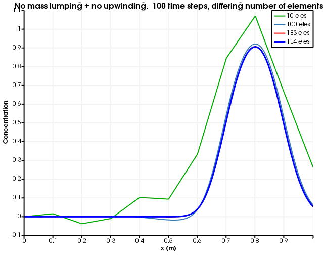
Figure 2: Diffusion as a function of number of elements. The number of time steps is fixed to 100 and no mass lumping and no upwinding is used.
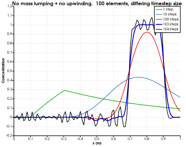
Figure 3: Diffusion as a function of number of time steps. The number of elements is fixed to 100 and no mass lumping and no upwinding is used.
Mass lumping and no upwinding
The MOOSE input file is:
# Using the fully-saturated action, which does mass lumping but no upwinding
[Mesh<<<{"href": "../../syntax/Mesh/index.html"}>>>]
  type = GeneratedMesh
  dim = 1
  nx = 100
  xmin = 0
  xmax = 1
[]

[GlobalParams<<<{"href": "../../syntax/GlobalParams/index.html"}>>>]
  PorousFlowDictator = dictator
[]

[Variables<<<{"href": "../../syntax/Variables/index.html"}>>>]
  [porepressure]
  []
  [tracer]
  []
[]

[ICs<<<{"href": "../../syntax/ICs/index.html"}>>>]
  [porepressure]
    type = FunctionIC<<<{"description": "An initial condition that uses a normal function of x, y, z to produce values (and optionally gradients) for a field variable.", "href": "../../source/ics/FunctionIC.html"}>>>
    variable<<<{"description": "The variable this initial condition is supposed to provide values for."}>>> = porepressure
    function<<<{"description": "The initial condition function."}>>> = '1 - x'
  []
  [tracer]
    type = FunctionIC<<<{"description": "An initial condition that uses a normal function of x, y, z to produce values (and optionally gradients) for a field variable.", "href": "../../source/ics/FunctionIC.html"}>>>
    variable<<<{"description": "The variable this initial condition is supposed to provide values for."}>>> = tracer
    function<<<{"description": "The initial condition function."}>>> = 'if(x<0.1,0,if(x>0.3,0,1))'
  []
[]

[PorousFlowFullySaturated<<<{"href": "../../syntax/PorousFlowFullySaturated/index.html"}>>>]
  porepressure<<<{"description": "The name of the porepressure variable"}>>> = porepressure
  coupling_type<<<{"description": "The type of simulation.  For simulations involving Mechanical deformations, you will need to supply the correct Biot coefficient.  For simulations involving Thermal flows, you will need an associated ConstantThermalExpansionCoefficient Material"}>>> = Hydro
  gravity<<<{"description": "Gravitational acceleration vector downwards (m/s^2)"}>>> = '0 0 0'
  fp<<<{"description": "The name of the user object for fluid properties. Only needed if fluid_properties_type = PorousFlowSingleComponentFluid"}>>> = the_simple_fluid
  mass_fraction_vars<<<{"description": "List of variables that represent the mass fractions.  With only one fluid component, this may be left empty.  With N fluid components, the format is 'f_0 f_1 f_2 ... f_(N-1)'.  That is, the N^th component need not be specified because f_N = 1 - (f_0 + f_1 + ... + f_(N-1)).  It is best numerically to choose the N-1 mass fraction variables so that they represent the fluid components with small concentrations.  This Action will associated the i^th mass fraction variable to the equation for the i^th fluid component, and the pressure variable to the N^th fluid component."}>>> = tracer
  stabilization<<<{"description": "Numerical stabilization used.  'Full' means full upwinding.  'KT' means FEM-TVD stabilization of Kuzmin-Turek"}>>> = none
[]

[BCs<<<{"href": "../../syntax/BCs/index.html"}>>>]
  [constant_injection_porepressure]
    type = DirichletBC<<<{"description": "Imposes the essential boundary condition $u=g$, where $g$ is a constant, controllable value.", "href": "../../source/bcs/DirichletBC.html"}>>>
    variable<<<{"description": "The name of the variable that this residual object operates on"}>>> = porepressure
    value<<<{"description": "Value of the BC"}>>> = 1
    boundary<<<{"description": "The list of boundary IDs from the mesh where this object applies"}>>> = left
  []
  [no_tracer_on_left]
    type = DirichletBC<<<{"description": "Imposes the essential boundary condition $u=g$, where $g$ is a constant, controllable value.", "href": "../../source/bcs/DirichletBC.html"}>>>
    variable<<<{"description": "The name of the variable that this residual object operates on"}>>> = tracer
    value<<<{"description": "Value of the BC"}>>> = 0
    boundary<<<{"description": "The list of boundary IDs from the mesh where this object applies"}>>> = left
  []
  [remove_component_1]
    type = PorousFlowPiecewiseLinearSink<<<{"description": "Applies a flux sink to a boundary. The base flux defined by PorousFlowSink is multiplied by a piecewise linear function.", "href": "../../source/bcs/PorousFlowPiecewiseLinearSink.html"}>>>
    variable<<<{"description": "The name of the variable that this residual object operates on"}>>> = porepressure
    boundary<<<{"description": "The list of boundary IDs from the mesh where this object applies"}>>> = right
    fluid_phase<<<{"description": "If supplied, then this BC will potentially be a function of fluid pressure, and you can use mass_fraction_component, use_mobility, use_relperm, use_enthalpy and use_energy.  If not supplied, then this BC can only be a function of temperature"}>>> = 0
    pt_vals<<<{"description": "Tuple of pressure values (for the fluid_phase specified).  Must be monotonically increasing.  For heat fluxes that don't involve fluids, these are temperature values"}>>> = '0 1E3'
    multipliers<<<{"description": "Tuple of multiplying values.  The flux values are multiplied by these."}>>> = '0 1E3'
    mass_fraction_component<<<{"description": "The index corresponding to a fluid component.  If supplied, the flux will be multiplied by the nodal mass fraction for the component"}>>> = 1
    use_mobility<<<{"description": "If true, then fluxes are multiplied by (density*permeability_nn/viscosity), where the '_nn' indicates the component normal to the boundary.  In this case bare_flux is measured in Pa.m^-1.  This can be used in conjunction with other use_*"}>>> = true
    flux_function<<<{"description": "The flux.  The flux is OUT of the medium: hence positive values of this function means this BC will act as a SINK, while negative values indicate this flux will be a SOURCE.  The functional form is useful for spatially or temporally varying sinks.  Without any use_*, this function is measured in kg.m^-2.s^-1 (or J.m^-2.s^-1 for the case with only heat and no fluids)"}>>> = 1E3
  []
  [remove_component_0]
    type = PorousFlowPiecewiseLinearSink<<<{"description": "Applies a flux sink to a boundary. The base flux defined by PorousFlowSink is multiplied by a piecewise linear function.", "href": "../../source/bcs/PorousFlowPiecewiseLinearSink.html"}>>>
    variable<<<{"description": "The name of the variable that this residual object operates on"}>>> = tracer
    boundary<<<{"description": "The list of boundary IDs from the mesh where this object applies"}>>> = right
    fluid_phase<<<{"description": "If supplied, then this BC will potentially be a function of fluid pressure, and you can use mass_fraction_component, use_mobility, use_relperm, use_enthalpy and use_energy.  If not supplied, then this BC can only be a function of temperature"}>>> = 0
    pt_vals<<<{"description": "Tuple of pressure values (for the fluid_phase specified).  Must be monotonically increasing.  For heat fluxes that don't involve fluids, these are temperature values"}>>> = '0 1E3'
    multipliers<<<{"description": "Tuple of multiplying values.  The flux values are multiplied by these."}>>> = '0 1E3'
    mass_fraction_component<<<{"description": "The index corresponding to a fluid component.  If supplied, the flux will be multiplied by the nodal mass fraction for the component"}>>> = 0
    use_mobility<<<{"description": "If true, then fluxes are multiplied by (density*permeability_nn/viscosity), where the '_nn' indicates the component normal to the boundary.  In this case bare_flux is measured in Pa.m^-1.  This can be used in conjunction with other use_*"}>>> = true
    flux_function<<<{"description": "The flux.  The flux is OUT of the medium: hence positive values of this function means this BC will act as a SINK, while negative values indicate this flux will be a SOURCE.  The functional form is useful for spatially or temporally varying sinks.  Without any use_*, this function is measured in kg.m^-2.s^-1 (or J.m^-2.s^-1 for the case with only heat and no fluids)"}>>> = 1E3
  []
[]

[FluidProperties<<<{"href": "../../syntax/FluidProperties/index.html"}>>>]
  [the_simple_fluid]
    type = SimpleFluidProperties<<<{"description": "Fluid properties for a simple fluid with a constant bulk density", "href": "../../source/fluidproperties/SimpleFluidProperties.html"}>>>
    bulk_modulus<<<{"description": "Constant bulk modulus (Pa)"}>>> = 2E9
    thermal_expansion<<<{"description": "Constant coefficient of thermal expansion (1/K)"}>>> = 0
    viscosity<<<{"description": "Constant dynamic viscosity (Pa.s)"}>>> = 1.0
    density0<<<{"description": "Density at zero pressure and zero temperature"}>>> = 1000.0
  []
[]

[Materials<<<{"href": "../../syntax/Materials/index.html"}>>>]
  [porosity]
    type = PorousFlowPorosity<<<{"description": "This Material calculates the porosity PorousFlow simulations", "href": "../../source/materials/PorousFlowPorosity.html"}>>>
    porosity_zero<<<{"description": "The porosity at zero volumetric strain and reference temperature and reference effective porepressure and reference chemistry.  This must be a real number or a constant monomial variable (not a linear lagrange or other type of variable)"}>>> = 0.1
  []
  [permeability]
    type = PorousFlowPermeabilityConst<<<{"description": "This Material calculates the permeability tensor assuming it is constant", "href": "../../source/materials/PorousFlowPermeabilityConst.html"}>>>
    permeability<<<{"description": "The permeability tensor (usually in m^2), which is assumed constant for this material"}>>> = '1E-2 0 0   0 1E-2 0   0 0 1E-2'
  []
[]

[Preconditioning<<<{"href": "../../syntax/Preconditioning/index.html"}>>>]
  active<<<{"description": "If specified only the blocks named will be visited and made active"}>>> = basic
  [basic]
    type = SMP<<<{"description": "Single matrix preconditioner (SMP) builds a preconditioner using user defined off-diagonal parts of the Jacobian.", "href": "../../source/preconditioners/SingleMatrixPreconditioner.html"}>>>
    full<<<{"description": "Set to true if you want the full set of couplings between variables simply for convenience so you don't have to set every off_diag_row and off_diag_column combination."}>>> = true
    petsc_options<<<{"description": "Singleton PETSc options"}>>> = '-ksp_diagonal_scale -ksp_diagonal_scale_fix'
    petsc_options_iname<<<{"description": "Names of PETSc name/value pairs"}>>> = '-pc_type -sub_pc_type -sub_pc_factor_shift_type -pc_asm_overlap'
    petsc_options_value<<<{"description": "Values of PETSc name/value pairs (must correspond with \"petsc_options_iname\""}>>> = ' asm      lu           NONZERO                   2'
  []
  [preferred_but_might_not_be_installed]
    type = SMP<<<{"description": "Single matrix preconditioner (SMP) builds a preconditioner using user defined off-diagonal parts of the Jacobian.", "href": "../../source/preconditioners/SingleMatrixPreconditioner.html"}>>>
    full<<<{"description": "Set to true if you want the full set of couplings between variables simply for convenience so you don't have to set every off_diag_row and off_diag_column combination."}>>> = true
    petsc_options_iname<<<{"description": "Names of PETSc name/value pairs"}>>> = '-pc_type -pc_factor_mat_solver_package'
    petsc_options_value<<<{"description": "Values of PETSc name/value pairs (must correspond with \"petsc_options_iname\""}>>> = ' lu       mumps'
  []
[]

[VectorPostprocessors<<<{"href": "../../syntax/VectorPostprocessors/index.html"}>>>]
  [tracer]
    type = LineValueSampler<<<{"description": "Samples variable(s) along a specified line", "href": "../../source/vectorpostprocessors/LineValueSampler.html"}>>>
    start_point<<<{"description": "The beginning of the line"}>>> = '0 0 0'
    end_point<<<{"description": "The ending of the line"}>>> = '1 0 0'
    num_points<<<{"description": "The number of points to sample along the line"}>>> = 101
    sort_by<<<{"description": "What to sort the samples by. Options include 'x', 'y', 'z', 'id', and the name of any of the sampled quantities (which each create a vector of the same name)."}>>> = x
    variable<<<{"description": "The names of the variables that this VectorPostprocessor operates on"}>>> = tracer
  []
[]

[Executioner<<<{"href": "../../syntax/Executioner/index.html"}>>>]
  type = Transient
  solve_type = Newton
  end_time = 6
  dt = 6E-1
  nl_abs_tol = 1E-8
  timestep_tolerance = 1E-3
[]

[Outputs<<<{"href": "../../syntax/Outputs/index.html"}>>>]
  [out]
    type = CSV<<<{"description": "Output for postprocessors, vector postprocessors, and scalar variables using comma seperated values (CSV).", "href": "../../source/outputs/CSV.html"}>>>
    execute_on<<<{"description": "The list of flag(s) indicating when this object should be executed. For a description of each flag, see https://mooseframework.inl.gov/source/interfaces/SetupInterface.html."}>>> = final
  []
[]Figure 4 and Figure 5 show the dependence on discretisation when there is no upwinding. Evidently, the lack of upwinding causes overshoots and undershoots, and the diffusion becomes less as the spatial discretisation becomes finer.
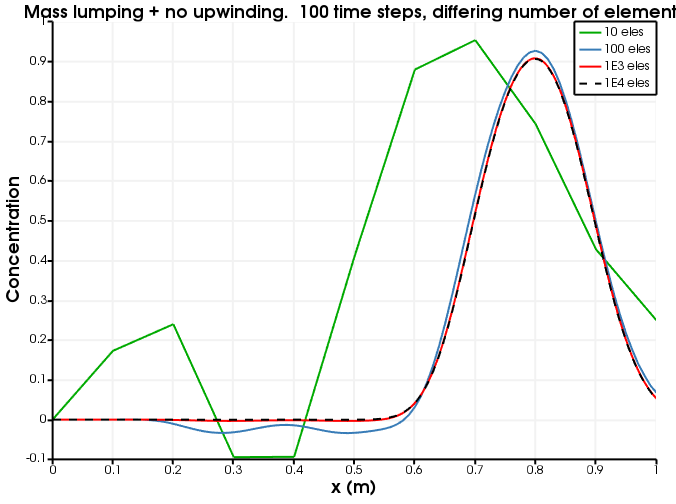
Figure 4: Diffusion as a function of number of elements. The number of time steps is fixed to 100 and no upwinding is used.
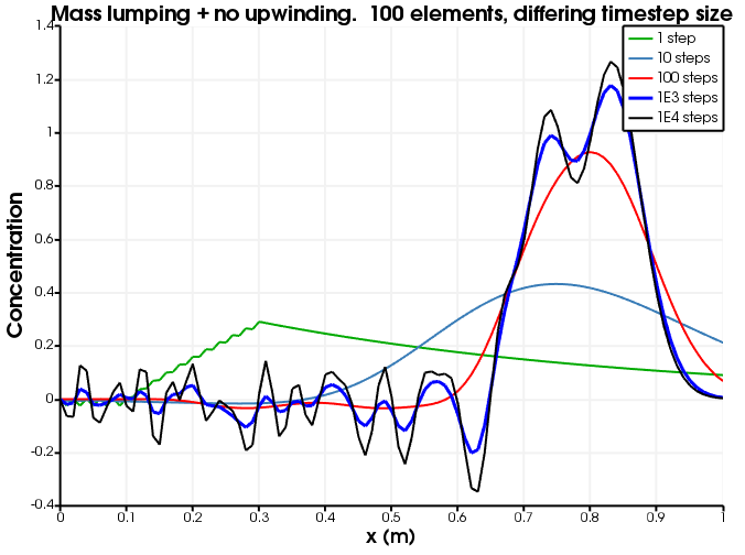
Figure 5: Diffusion as a function of number of time steps. The number of elements is fixed to 100 and no upwinding is used.
Mass lumping and full upwinding
The MOOSE input file is identical to the one above, save for the PorousFlowFullySaturated block that must now contain stabilization = Full:
[PorousFlowFullySaturated]
  porepressure = porepressure
  coupling_type = Hydro
  gravity = '0 0 0'
  fp = the_simple_fluid
  mass_fraction_vars = tracer
  stabilization = Full
[]
(Also, the test suite contains a non-action version).
Figure 6 and Figure 7 show the dependence on discretisation when full upwinding is used.
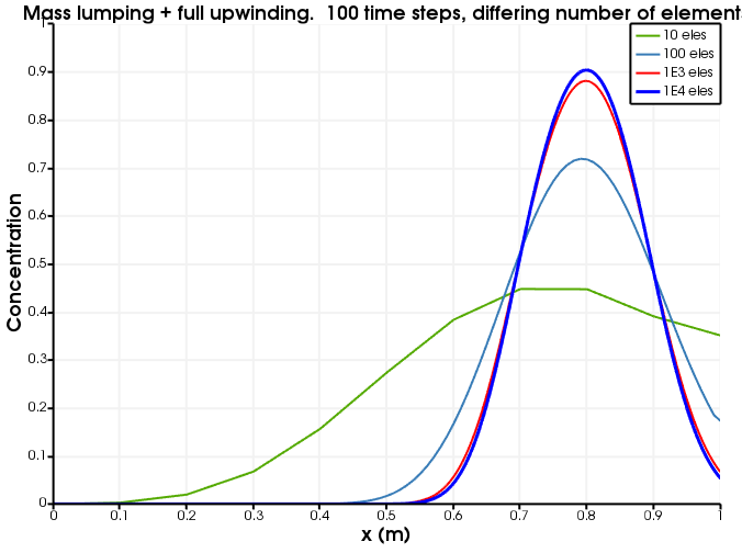
Figure 6: Diffusion as a function of number of elements. The number of time steps is fixed to 100 and full upwinding is used.
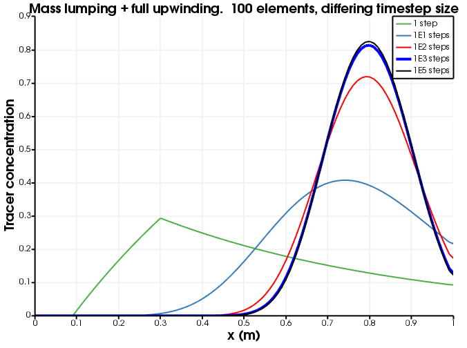
Figure 7: Diffusion as a function of number of time steps. The number of elements is fixed to 100 and full upwinding is used.
RDG(P0)
In RDG, the variables (just the tracer in this case) are constant-monomial, that is, they are constant throughout the element. This means MOOSE behaves like a Finite Volume Method, and it means that the output looks less smooth than the usual linear-Lagrange variables (the figures below display "stepped" results). The MOOSE input file is:
# This test demonstrates the advection of a tracer in 1D using the RDG module.
# There is no slope limiting.  Changing the SlopeLimiting scheme to minmod, mc,
# or superbee means that a linear reconstruction is performed, and the slope
# limited according to the scheme chosen.  Doing this produces RDG(P0P1) and
# substantially reduces numerical diffusion

[Mesh<<<{"href": "../../syntax/Mesh/index.html"}>>>]
  type = GeneratedMesh
  dim = 1
  nx = 100
  xmin = 0
  xmax = 1
[]

[Variables<<<{"href": "../../syntax/Variables/index.html"}>>>]
  [./tracer]
    order<<<{"description": "Specifies the order of the FE shape function to use for this variable (additional orders not listed are allowed)"}>>> = CONSTANT
    family<<<{"description": "Specifies the family of FE shape functions to use for this variable"}>>> = MONOMIAL
  [../]
[]

[ICs<<<{"href": "../../syntax/ICs/index.html"}>>>]
  [./tracer]
    type = FunctionIC<<<{"description": "An initial condition that uses a normal function of x, y, z to produce values (and optionally gradients) for a field variable.", "href": "../../source/ics/FunctionIC.html"}>>>
    variable<<<{"description": "The variable this initial condition is supposed to provide values for."}>>> = tracer
    function<<<{"description": "The initial condition function."}>>> = 'if(x<0.1,0,if(x>0.3,0,1))'
  [../]
[]

[UserObjects<<<{"href": "../../syntax/UserObjects/index.html"}>>>]
  [./lslope]
    type = AEFVSlopeLimitingOneD<<<{"description": "One-dimensional slope limiting to get the limited slope of cell average variable for the advection equation using a cell-centered finite volume method.", "href": "../../source/userobjects/AEFVSlopeLimitingOneD.html"}>>>
    execute_on<<<{"description": "The list of flag(s) indicating when this object should be executed. For a description of each flag, see https://mooseframework.inl.gov/source/interfaces/SetupInterface.html."}>>> = 'linear'
    scheme<<<{"description": "TVD-type slope limiting scheme"}>>> = 'none' #none | minmod | mc | superbee
    u<<<{"description": "constant monomial variable"}>>> = tracer
  [../]

  [./internal_side_flux]
    type = AEFVUpwindInternalSideFlux<<<{"description": "Upwind numerical flux scheme for the advection equation using a cell-centered finite volume method.", "href": "../../source/userobjects/AEFVUpwindInternalSideFlux.html"}>>>
    execute_on<<<{"description": "The list of flag(s) indicating when this object should be executed. For a description of each flag, see https://mooseframework.inl.gov/source/interfaces/SetupInterface.html."}>>> = 'linear'
    velocity<<<{"description": "Advective velocity"}>>> = 0.1
  [../]

  [./free_outflow_bc]
    type = AEFVFreeOutflowBoundaryFlux<<<{"description": "Free outflow BC based boundary flux user object for the advection equation using a cell-centered finite volume method.", "href": "../../source/userobjects/AEFVFreeOutflowBoundaryFlux.html"}>>>
    execute_on<<<{"description": "The list of flag(s) indicating when this object should be executed. For a description of each flag, see https://mooseframework.inl.gov/source/interfaces/SetupInterface.html."}>>> = 'linear'
    velocity<<<{"description": "Advective velocity"}>>> = 0.1
  [../]
[]

[Kernels<<<{"href": "../../syntax/Kernels/index.html"}>>>]
  [./dot]
    type = TimeDerivative<<<{"description": "The time derivative operator with the weak form of $(\\psi_i, \\frac{\\partial u_h}{\\partial t})$.", "href": "../../source/kernels/TimeDerivative.html"}>>>
    variable<<<{"description": "The name of the variable that this residual object operates on"}>>> = tracer
  [../]
[]
[DGKernels<<<{"href": "../../syntax/DGKernels/index.html"}>>>]
  [./concentration]
    type = AEFVKernel<<<{"description": "A dgkernel for the advection equation using a cell-centered finite volume method.", "href": "../../source/dgkernels/AEFVKernel.html"}>>>
    variable<<<{"description": "The name of the variable that this residual object operates on"}>>> = tracer
    component<<<{"description": "Choose one of the equations"}>>> = 'concentration'
    flux<<<{"description": "Name of the internal side flux object to use"}>>> = internal_side_flux
    u<<<{"description": "Name of the variable to use"}>>> = tracer
  [../]
[]

[BCs<<<{"href": "../../syntax/BCs/index.html"}>>>]
  [./concentration]
    type = AEFVBC<<<{"description": "A boundary condition kernel for the advection equation using a cell-centered finite volume method.", "href": "../../source/bcs/AEFVBC.html"}>>>
    boundary<<<{"description": "The list of boundary IDs from the mesh where this object applies"}>>> = 'left right'
    variable<<<{"description": "The name of the variable that this residual object operates on"}>>> = tracer
    component<<<{"description": "Choose one of the equations"}>>> = 'concentration'
    flux<<<{"description": "Name of the boundary flux object to use"}>>> = free_outflow_bc
    u<<<{"description": "Name of the variable to use"}>>> = tracer
  [../]
[]

[Materials<<<{"href": "../../syntax/Materials/index.html"}>>>]
  [./aefv]
    type = AEFVMaterial<<<{"description": "A material kernel for the advection equation using a cell-centered finite volume method.", "href": "../../source/materials/AEFVMaterial.html"}>>>
    slope_limiting<<<{"description": "Name for slope limiting user object"}>>> = lslope
    u<<<{"description": "Cell-averge variable"}>>> = tracer
  [../]
[]

[VectorPostprocessors<<<{"href": "../../syntax/VectorPostprocessors/index.html"}>>>]
  [./tracer]
    type = LineValueSampler<<<{"description": "Samples variable(s) along a specified line", "href": "../../source/vectorpostprocessors/LineValueSampler.html"}>>>
    start_point<<<{"description": "The beginning of the line"}>>> = '0 0 0'
    end_point<<<{"description": "The ending of the line"}>>> = '1 0 0'
    num_points<<<{"description": "The number of points to sample along the line"}>>> = 100
    sort_by<<<{"description": "What to sort the samples by. Options include 'x', 'y', 'z', 'id', and the name of any of the sampled quantities (which each create a vector of the same name)."}>>> = x
    variable<<<{"description": "The names of the variables that this VectorPostprocessor operates on"}>>> = tracer
  [../]
[]

[Executioner<<<{"href": "../../syntax/Executioner/index.html"}>>>]
  type = Transient
  solve_type = PJFNK
  end_time = 6
  dt = 6E-1
  nl_abs_tol = 1E-8
  timestep_tolerance = 1E-3
[]

[Outputs<<<{"href": "../../syntax/Outputs/index.html"}>>>]
  #exodus = true
  csv<<<{"description": "Output the scalar variable and postprocessors to a *.csv file using the default CSV output."}>>> = true
  execute_on<<<{"description": "The list of flag(s) indicating when this object should be executed. For a description of each flag, see https://mooseframework.inl.gov/source/interfaces/SetupInterface.html."}>>> = final
[]Figure 8 and Figure 9 show the dependence on discretisation when RDG(P0) is used. This is identical to mass-lumping + full-upwinding (up to the fact that constant-monomial variables are used instead of linear-Lagrange). As expected, there are no oscillations or over-shoots or under-shoots, but the results suffer from numerical diffusion.
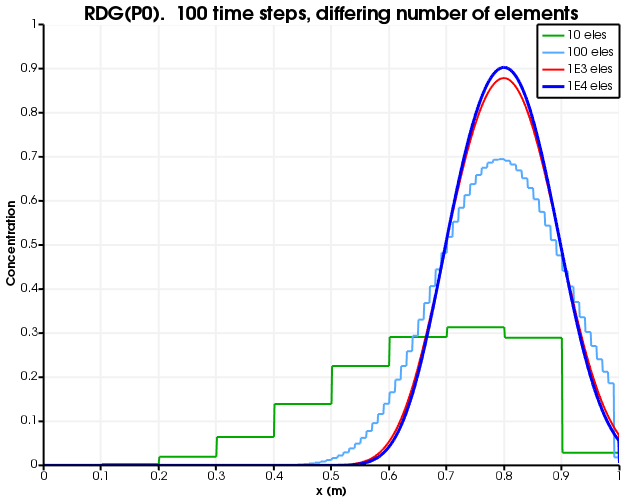
Figure 8: Diffusion as a function of number of elements. The number of time steps is fixed to 100 and RDG(P0) is used.
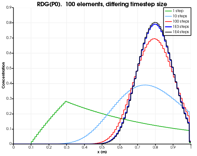
Figure 9: Diffusion as a function of number of time steps. The number of elements is fixed to 100 and RDG(P0) is used.
RDG(P0P1)
The MOOSE input file is almost identical to the RDG(P0) version, save for the changing the SlopeLimiting scheme from "none" to "mc" (or another limiter such as "minmod" or "superbee").
Figure 10 and Figure 11 show the dependence on discretisation when RDG(P0P1) is used. As with RDG(P0), there are no oscillations or over-shoots or under-shoots. However, numerical diffusion is greatly reduced by the linear reconstruction.
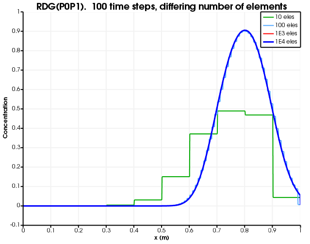
Figure 10: Diffusion as a function of number of elements. The number of time steps is fixed to 100 and RDG(P0P1) is used.
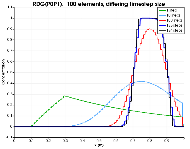
Figure 11: Diffusion as a function of number of time steps. The number of elements is fixed to 100 and RDG(P0P1) is used.
Kuzmin-Turek scheme with no flux limiter
To employ the Kuzmin-Turek scheme, the fully_saturated_action.i input file listed above may be simply modified by including KT stabilization:
[PorousFlowFullySaturated]
  porepressure = porepressure
  coupling_type = Hydro
  gravity = '0 0 0'
  fp = the_simple_fluid
  mass_fraction_vars = tracer
  stabilization = KT
  flux_limiter_type = None
[]
in the PorousFlowFullySaturated Action block. Alternatively, a new input file may be built, such as:
# Using Flux-Limited TVD Advection ala Kuzmin and Turek, but without any antidiffusion
[Mesh<<<{"href": "../../syntax/Mesh/index.html"}>>>]
  type = GeneratedMesh
  dim = 1
  nx = 100
  xmin = 0
  xmax = 1
[]

[Variables<<<{"href": "../../syntax/Variables/index.html"}>>>]
  [tracer]
  []
[]

[ICs<<<{"href": "../../syntax/ICs/index.html"}>>>]
  [tracer]
    type = FunctionIC<<<{"description": "An initial condition that uses a normal function of x, y, z to produce values (and optionally gradients) for a field variable.", "href": "../../source/ics/FunctionIC.html"}>>>
    variable<<<{"description": "The variable this initial condition is supposed to provide values for."}>>> = tracer
    function<<<{"description": "The initial condition function."}>>> = 'if(x<0.1,0,if(x>0.3,0,1))'
  []
[]

[Kernels<<<{"href": "../../syntax/Kernels/index.html"}>>>]
  [mass_dot]
    type = MassLumpedTimeDerivative<<<{"description": "Lumped formulation of the time derivative $\\frac{\\partial u}{\\partial t}$. Its corresponding weak form is $\\dot{u_i}(\\psi_i, 1)$ where $\\dot{u_i}$ denotes the time derivative of the solution coefficient associated with node $i$.", "href": "../../source/kernels/MassLumpedTimeDerivative.html"}>>>
    variable<<<{"description": "The name of the variable that this residual object operates on"}>>> = tracer
  []
  [flux]
    type = FluxLimitedTVDAdvection<<<{"description": "Conservative form of $\\nabla \\cdot \\vec{v} u$ (advection), using the Flux Limited TVD scheme invented by Kuzmin and Turek", "href": "../../source/kernels/FluxLimitedTVDAdvection.html"}>>>
    variable<<<{"description": "The name of the variable that this residual object operates on"}>>> = tracer
    advective_flux_calculator<<<{"description": "AdvectiveFluxCalculator UserObject"}>>> = fluo
  []
[]

[UserObjects<<<{"href": "../../syntax/UserObjects/index.html"}>>>]
  [fluo]
    type = AdvectiveFluxCalculatorConstantVelocity<<<{"description": "Compute K_ij (a measure of advective flux from node i to node j) and R+ and R- (which quantify amount of antidiffusion to add) in the Kuzmin-Turek FEM-TVD multidimensional scheme.  Constant advective velocity is assumed", "href": "../../source/userobjects/AdvectiveFluxCalculatorConstantVelocity.html"}>>>
    flux_limiter_type<<<{"description": "Type of flux limiter to use.  'None' means that no antidiffusion will be added in the Kuzmin-Turek scheme"}>>> = none
    u<<<{"description": "The variable that is being advected"}>>> = tracer
    velocity<<<{"description": "Velocity vector"}>>> = '0.1 0 0'
  []
[]

[BCs<<<{"href": "../../syntax/BCs/index.html"}>>>]
  [no_tracer_on_left]
    type = DirichletBC<<<{"description": "Imposes the essential boundary condition $u=g$, where $g$ is a constant, controllable value.", "href": "../../source/bcs/DirichletBC.html"}>>>
    variable<<<{"description": "The name of the variable that this residual object operates on"}>>> = tracer
    value<<<{"description": "Value of the BC"}>>> = 0
    boundary<<<{"description": "The list of boundary IDs from the mesh where this object applies"}>>> = left
  []
  [remove_tracer]
# Ideally, an OutflowBC would be used, but that does not exist in the framework
# In 1D VacuumBC is the same as OutflowBC, with the alpha parameter being twice the velocity
    type = VacuumBC<<<{"description": "Vacuum boundary condition for diffusion.", "href": "../../source/bcs/VacuumBC.html"}>>>
    boundary<<<{"description": "The list of boundary IDs from the mesh where this object applies"}>>> = right
    alpha<<<{"description": "Diffusion coefficient."}>>> = 0.2 # 2 * velocity
    variable<<<{"description": "The name of the variable that this residual object operates on"}>>> = tracer
  []
[]

[Preconditioning<<<{"href": "../../syntax/Preconditioning/index.html"}>>>]
  active<<<{"description": "If specified only the blocks named will be visited and made active"}>>> = basic
  [basic]
    type = SMP<<<{"description": "Single matrix preconditioner (SMP) builds a preconditioner using user defined off-diagonal parts of the Jacobian.", "href": "../../source/preconditioners/SingleMatrixPreconditioner.html"}>>>
    full<<<{"description": "Set to true if you want the full set of couplings between variables simply for convenience so you don't have to set every off_diag_row and off_diag_column combination."}>>> = true
    petsc_options<<<{"description": "Singleton PETSc options"}>>> = '-ksp_diagonal_scale -ksp_diagonal_scale_fix'
    petsc_options_iname<<<{"description": "Names of PETSc name/value pairs"}>>> = '-pc_type -sub_pc_type -sub_pc_factor_shift_type -pc_asm_overlap'
    petsc_options_value<<<{"description": "Values of PETSc name/value pairs (must correspond with \"petsc_options_iname\""}>>> = ' asm      lu           NONZERO                   2'
  []
  [preferred_but_might_not_be_installed]
    type = SMP<<<{"description": "Single matrix preconditioner (SMP) builds a preconditioner using user defined off-diagonal parts of the Jacobian.", "href": "../../source/preconditioners/SingleMatrixPreconditioner.html"}>>>
    full<<<{"description": "Set to true if you want the full set of couplings between variables simply for convenience so you don't have to set every off_diag_row and off_diag_column combination."}>>> = true
    petsc_options_iname<<<{"description": "Names of PETSc name/value pairs"}>>> = '-pc_type -pc_factor_mat_solver_package'
    petsc_options_value<<<{"description": "Values of PETSc name/value pairs (must correspond with \"petsc_options_iname\""}>>> = ' lu       mumps'
  []
[]

[VectorPostprocessors<<<{"href": "../../syntax/VectorPostprocessors/index.html"}>>>]
  [tracer]
    type = LineValueSampler<<<{"description": "Samples variable(s) along a specified line", "href": "../../source/vectorpostprocessors/LineValueSampler.html"}>>>
    start_point<<<{"description": "The beginning of the line"}>>> = '0 0 0'
    end_point<<<{"description": "The ending of the line"}>>> = '1 0 0'
    num_points<<<{"description": "The number of points to sample along the line"}>>> = 101
    sort_by<<<{"description": "What to sort the samples by. Options include 'x', 'y', 'z', 'id', and the name of any of the sampled quantities (which each create a vector of the same name)."}>>> = x
    variable<<<{"description": "The names of the variables that this VectorPostprocessor operates on"}>>> = tracer
  []
[]

[Executioner<<<{"href": "../../syntax/Executioner/index.html"}>>>]
  type = Transient
  solve_type = Newton
  end_time = 6
  dt = 6E-1
  nl_abs_tol = 1E-8
  nl_max_its = 500
  timestep_tolerance = 1E-3
[]

[Outputs<<<{"href": "../../syntax/Outputs/index.html"}>>>]
  [out]
    type = CSV<<<{"description": "Output for postprocessors, vector postprocessors, and scalar variables using comma seperated values (CSV).", "href": "../../source/outputs/CSV.html"}>>>
    execute_on<<<{"description": "The list of flag(s) indicating when this object should be executed. For a description of each flag, see https://mooseframework.inl.gov/source/interfaces/SetupInterface.html."}>>> = final
  []
[]Figure 12 and Figure 13 show the dependence on discretisation when Kuzmin-Turek with no flux limiter is used. As expected, the behaviour is identical to the case with full upwinding.
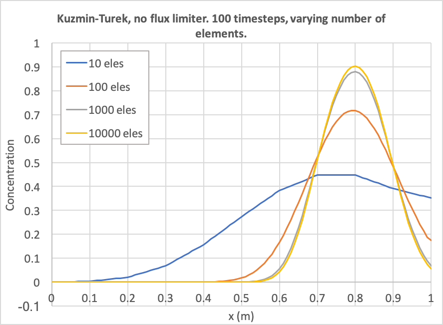
Figure 12: Diffusion as a function of number of elements. The number of time steps is fixed to 100 and Kuzmin-Turek with no flux limiter is used.
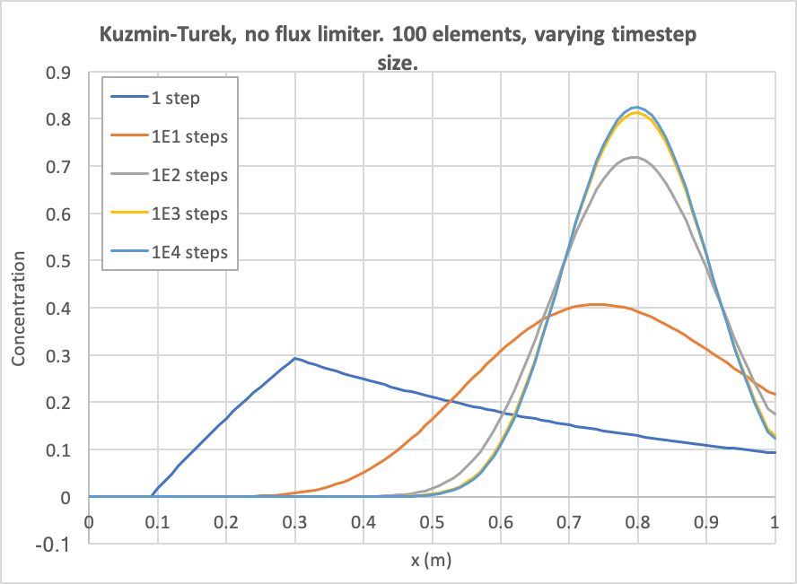
Figure 13: Diffusion as a function of number of time steps. The number of elements is fixed to 100 and Kuzmin-Turek with no flux limiter is used.
Kuzmin-Turek scheme with flux limiter
To employ the Kuzmin-Turek scheme, the fully_saturated_action.i input file listed above may be simply modified by including KT stabilization:
[PorousFlowFullySaturated]
  porepressure = porepressure
  coupling_type = Hydro
  gravity = '0 0 0'
  fp = the_simple_fluid
  mass_fraction_vars = tracer
  stabilization = KT
  flux_limiter_type = superbee
[]
in the PorousFlowFullySaturated Action block. Alternatively, a new input file may be built, such as:
# Using Flux-Limited TVD Advection ala Kuzmin and Turek, with antidiffusion from superbee flux limiting
[Mesh<<<{"href": "../../syntax/Mesh/index.html"}>>>]
  type = GeneratedMesh
  dim = 1
  nx = 100
  xmin = 0
  xmax = 1
[]

[Variables<<<{"href": "../../syntax/Variables/index.html"}>>>]
  [tracer]
  []
[]

[ICs<<<{"href": "../../syntax/ICs/index.html"}>>>]
  [tracer]
    type = FunctionIC<<<{"description": "An initial condition that uses a normal function of x, y, z to produce values (and optionally gradients) for a field variable.", "href": "../../source/ics/FunctionIC.html"}>>>
    variable<<<{"description": "The variable this initial condition is supposed to provide values for."}>>> = tracer
    function<<<{"description": "The initial condition function."}>>> = 'if(x<0.1,0,if(x>0.3,0,1))'
  []
[]

[Kernels<<<{"href": "../../syntax/Kernels/index.html"}>>>]
  [mass_dot]
    type = MassLumpedTimeDerivative<<<{"description": "Lumped formulation of the time derivative $\\frac{\\partial u}{\\partial t}$. Its corresponding weak form is $\\dot{u_i}(\\psi_i, 1)$ where $\\dot{u_i}$ denotes the time derivative of the solution coefficient associated with node $i$.", "href": "../../source/kernels/MassLumpedTimeDerivative.html"}>>>
    variable<<<{"description": "The name of the variable that this residual object operates on"}>>> = tracer
  []
  [flux]
    type = FluxLimitedTVDAdvection<<<{"description": "Conservative form of $\\nabla \\cdot \\vec{v} u$ (advection), using the Flux Limited TVD scheme invented by Kuzmin and Turek", "href": "../../source/kernels/FluxLimitedTVDAdvection.html"}>>>
    variable<<<{"description": "The name of the variable that this residual object operates on"}>>> = tracer
    advective_flux_calculator<<<{"description": "AdvectiveFluxCalculator UserObject"}>>> = fluo
  []
[]

[UserObjects<<<{"href": "../../syntax/UserObjects/index.html"}>>>]
  [fluo]
    type = AdvectiveFluxCalculatorConstantVelocity<<<{"description": "Compute K_ij (a measure of advective flux from node i to node j) and R+ and R- (which quantify amount of antidiffusion to add) in the Kuzmin-Turek FEM-TVD multidimensional scheme.  Constant advective velocity is assumed", "href": "../../source/userobjects/AdvectiveFluxCalculatorConstantVelocity.html"}>>>
    flux_limiter_type<<<{"description": "Type of flux limiter to use.  'None' means that no antidiffusion will be added in the Kuzmin-Turek scheme"}>>> = superbee
    u<<<{"description": "The variable that is being advected"}>>> = tracer
    velocity<<<{"description": "Velocity vector"}>>> = '0.1 0 0'
  []
[]

[BCs<<<{"href": "../../syntax/BCs/index.html"}>>>]
  [no_tracer_on_left]
    type = DirichletBC<<<{"description": "Imposes the essential boundary condition $u=g$, where $g$ is a constant, controllable value.", "href": "../../source/bcs/DirichletBC.html"}>>>
    variable<<<{"description": "The name of the variable that this residual object operates on"}>>> = tracer
    value<<<{"description": "Value of the BC"}>>> = 0
    boundary<<<{"description": "The list of boundary IDs from the mesh where this object applies"}>>> = left
  []
  [remove_tracer]
# Ideally, an OutflowBC would be used, but that does not exist in the framework
# In 1D VacuumBC is the same as OutflowBC, with the alpha parameter being twice the velocity
    type = VacuumBC<<<{"description": "Vacuum boundary condition for diffusion.", "href": "../../source/bcs/VacuumBC.html"}>>>
    boundary<<<{"description": "The list of boundary IDs from the mesh where this object applies"}>>> = right
    alpha<<<{"description": "Diffusion coefficient."}>>> = 0.2 # 2 * velocity
    variable<<<{"description": "The name of the variable that this residual object operates on"}>>> = tracer
  []
[]

[Preconditioning<<<{"href": "../../syntax/Preconditioning/index.html"}>>>]
  active<<<{"description": "If specified only the blocks named will be visited and made active"}>>> = basic
  [basic]
    type = SMP<<<{"description": "Single matrix preconditioner (SMP) builds a preconditioner using user defined off-diagonal parts of the Jacobian.", "href": "../../source/preconditioners/SingleMatrixPreconditioner.html"}>>>
    full<<<{"description": "Set to true if you want the full set of couplings between variables simply for convenience so you don't have to set every off_diag_row and off_diag_column combination."}>>> = true
    petsc_options<<<{"description": "Singleton PETSc options"}>>> = '-ksp_diagonal_scale -ksp_diagonal_scale_fix'
    petsc_options_iname<<<{"description": "Names of PETSc name/value pairs"}>>> = '-pc_type -sub_pc_type -sub_pc_factor_shift_type -pc_asm_overlap'
    petsc_options_value<<<{"description": "Values of PETSc name/value pairs (must correspond with \"petsc_options_iname\""}>>> = ' asm      lu           NONZERO                   2'
  []
  [preferred_but_might_not_be_installed]
    type = SMP<<<{"description": "Single matrix preconditioner (SMP) builds a preconditioner using user defined off-diagonal parts of the Jacobian.", "href": "../../source/preconditioners/SingleMatrixPreconditioner.html"}>>>
    full<<<{"description": "Set to true if you want the full set of couplings between variables simply for convenience so you don't have to set every off_diag_row and off_diag_column combination."}>>> = true
    petsc_options_iname<<<{"description": "Names of PETSc name/value pairs"}>>> = '-pc_type -pc_factor_mat_solver_package'
    petsc_options_value<<<{"description": "Values of PETSc name/value pairs (must correspond with \"petsc_options_iname\""}>>> = ' lu       mumps'
  []
[]

[VectorPostprocessors<<<{"href": "../../syntax/VectorPostprocessors/index.html"}>>>]
  [tracer]
    type = LineValueSampler<<<{"description": "Samples variable(s) along a specified line", "href": "../../source/vectorpostprocessors/LineValueSampler.html"}>>>
    start_point<<<{"description": "The beginning of the line"}>>> = '0 0 0'
    end_point<<<{"description": "The ending of the line"}>>> = '1 0 0'
    num_points<<<{"description": "The number of points to sample along the line"}>>> = 101
    sort_by<<<{"description": "What to sort the samples by. Options include 'x', 'y', 'z', 'id', and the name of any of the sampled quantities (which each create a vector of the same name)."}>>> = x
    variable<<<{"description": "The names of the variables that this VectorPostprocessor operates on"}>>> = tracer
  []
[]

[Executioner<<<{"href": "../../syntax/Executioner/index.html"}>>>]
  type = Transient
  solve_type = Newton
  end_time = 6
  dt = 6E-2
  nl_abs_tol = 1E-8
  nl_max_its = 500
  timestep_tolerance = 1E-3
[]

[Outputs<<<{"href": "../../syntax/Outputs/index.html"}>>>]
  [out]
    type = CSV<<<{"description": "Output for postprocessors, vector postprocessors, and scalar variables using comma seperated values (CSV).", "href": "../../source/outputs/CSV.html"}>>>
    execute_on<<<{"description": "The list of flag(s) indicating when this object should be executed. For a description of each flag, see https://mooseframework.inl.gov/source/interfaces/SetupInterface.html."}>>> = final
  []
[]Figure 14 and Figure 15 show the dependence on discretisation when Kuzmin-Turek with a flux limiter is used (the "superbee" limiter has been chosen in this case, see the worked example of Kuzmin-Turek stabilization). As expected, the behaviour is similar to the RDG(POP1) case, except it is smooth because the variables are linear-lagrange.
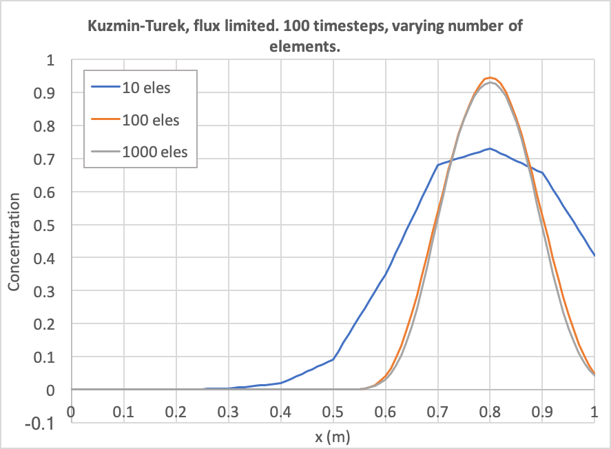
Figure 14: Diffusion as a function of number of elements. The number of time steps is fixed to 100 and Kuzmin-Turek with the superbee flux limiter.
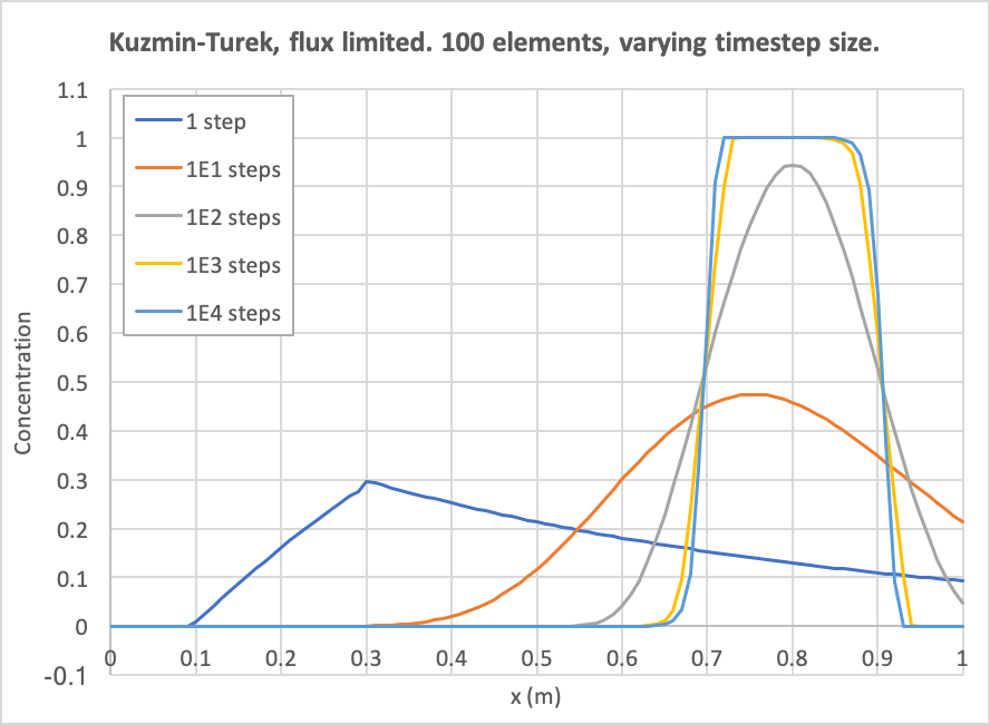
Figure 15: Diffusion as a function of number of time steps. The number of elements is fixed to 100 and Kuzmin-Turek with the superbee flux limiter.
Summary
By way of comparison, Figure 16 and Figure 17 show the results when the number of elements is fixed to 100 and the number of timesteps is 100 or 1000 (respectively). Evidently, without upwinding, the result includes over-shoots and under-shoots, which are typically devastating for PorousFlow simulations, since they typically manifest themselves as negative saturations, negative mass fractions, or negative temperatures. With upwinding, RDG(P0), or Kuzmin-Turek with no antidiffusion these are avoided, at the expense of introducing large numerical diffusion. RDG(P0P1) and Kuzmin-Turek with a flux limiter produces a similar amount of numerical diffusion to the non-upwinded, non-masslumped version, but without introducing any over-shoots and under-shoots.
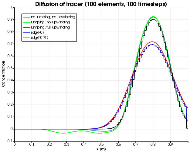
Figure 16: Diffusion for different numerical schemes. 100 timesteps are used.
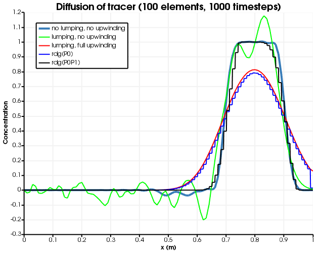
Figure 17: Diffusion for different numerical schemes. 1000 timesteps are used.
Interestingly, as the timestep size is decreased, the numerical diffusion is decreased when using lumping and upwinding, but only up to a point: increasing the number of timesteps from 100 to 10000 makes basically no difference when the number of elements is 100. This suggests that lumping and full-upwinding will always produce numerical diffusion, and this may be proved by simple analysis (not presented here) since the tracer always gets moved from upwind node to downwind node irrespective of the concentration of the tracer.