Theory manual
Introduction
Multi-hazard Analysis for STOchastic time-DOmaiN phenomena (MASTODON) is a finite element application that aims at analyzing the response of 3-D soil-structure systems to natural and man-made hazards such as earthquakes, floods and fire. MASTODON currently focuses on the simulation of seismic events and has the capability to perform extensive 'source-to-site' simulations including earthquake fault rupture, nonlinear wave propagation and nonlinear soil-structure interaction (NLSSI) analysis. MASTODON is being developed to be a dynamic probabilistic risk assessment framework that enables analysts to not only perform deterministic analyses, but also easily perform probabilistic or stochastic simulations for the purpose of risk assessment.
MASTODON is a MOOSE-based application and performs finite-element analysis of the dynamics of solids, mechanics of interfaces and porous media flow. It is equipped with effective stress space nonlinear hysteretic soil constitutive model (I-soil), and a u-p-U formulation to couple solid and fluid, as well as structural materials such as reinforced concrete. It includes interface models that simulate gapping, sliding and uplift at the interfaces of solid media such as the foundation-soil interface of structures. Absorbing boundary models for the simulation of infinite or semi-infinite domains, fault rupture model for seismic source simulation, and the domain reduction method for the input of complex, three-dimensional wave fields are incorporated. Since MASTODON is a MOOSE-based application, it can efficiently solve problems using standard workstations or very large high-performance computers.
This document describes the theoretical and numerical foundations of MASTODON.
Units
MASTODON does not follow a fixed unit system unless explicitly specified in the corresponding syntax, user manual or theory manual. Users should ensure that the quantities specified in the input file follow a consistent set of units.
Governing equations
The basic equation that MASTODON solves is the nonlinear wave equation:
(1)
where, is the density of the soil or structure that can vary with space, is the stress at any point in space and time, is the external force acting on the system that can be in the form of localized seismic sources or global body forces such as gravity, and is the acceleration at any point within the soil-structure domain. The left side of the equation contains the internal forces acting on the system with first term being the contribution from the inertia, and the second term being the contribution from the stiffness of the system. Additional terms would be added to this equation when damping is present in the system. The material stress response () is described by the constitutive model, where the stress is determined as a function of the strain (), i.e. . Details about the material constitutive models available in MASTODON are presented in the section about material models.
The above equation is incomplete and ill-conditioned without the corresponding boundary conditions. There are two main types of boundary conditions: (i) Dirichlet boundary condition which is a kinematic boundary condition where the displacement, velocity, or acceleration at that boundary is specified; (ii) Neumann boundary condition where a force or traction is applied at the boundary. All the special boundary conditions such as absorbing boundary condition are specialized versions of these broad boundary condition types.
Time integration
To solve the governing equation above for , an appropriate time integration scheme needs to be chosen. Newmark and Hilber-Hughes-Taylor (HHT) time integration schemes are two of the commonly used methods in solving wave propagation problems.
Newmark time integration
In Newmark time integration (Newmark, 1959), the acceleration and velocity at are written in terms of the displacement (), velocity () and acceleration () at time and the displacement at .
(2)
In the above equations, and are Newmark time integration parameters. Substituting the above two equations into the equation of motion will result in a linear system of equations () from which can be estimated.
For and , the Newmark time integration scheme is the same as the trapezoidal rule. The trapezoidal rule is an unconditionally stable integration scheme, i.e., the solution does not diverge for any choice of , and the solution obtained from this scheme is second order accurate. One disadvantage with using trapezoidal rule is the absence of numerical damping to damp out any high frequency numerical noise that is generated due to the discretization of the equation of motion in time.
The Newmark time integration scheme is unconditionally stable for and . For , high frequency oscillations are damped out, but the solution accuracy decreases to first order.
Damping
When the soil-structure system (including both soil and concrete) responds to an earthquake excitation, energy is dissipated in two primary ways: (1)small-strain and hysteretic material damping, and (2) damping due to gapping, sliding and uplift at the soil-foundation interface. Dissipation of energy due to item (1) is modeled (approximately) using following methods: (i) viscous damping for small strain damping experienced at very small strain levels ( ) where the material behavior is largely linear viscoelastic; (ii) hysteretic damping due to nonlinear hysteretic behavior of the material. Dissipation of energy due to (2) is discussed in the foundation-soil interface section. This section discusses the damping that is present at small strain levels.
Rayleigh damping
Rayleigh damping is the most common form of classical damping used in modeling structural dynamic problems. The more generalized form of classical damping, Caughey Damping (Caughey, 1960), is currently not implemented in MASTODON. Rayleigh damping is a specific form of Caughey damping that uses only the first two terms of the series. In this method, the viscous damping is proportional to the inertial contribution and contribution from the stiffness. This implies that in the matrix form of the governing equation, the damping matrix () is assumed to be a linear combination of the mass () and stiffness () matrices, i.e., . Here, and are the mass and stiffness dependent Rayleigh damping parameters, respectively.
The equation of motion (in the matrix form) in the presence of Rayleigh damping becomes:
The same equation of motion at any point in space and time (in the non-matrix form) is given by:
The degree of damping in the system depends on the coefficients and as follows: (3)
where, is the damping ratio of the system as a function of frequency . The damping ratio as a function of frequency for and is presented in Figure 1.
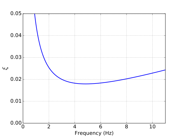
Figure 1: Damping ratio as a function of frequency.
Simulation of a constant damping ratio
For the constant damping ratio scenario, the aim is to find and such that the is close to the target damping ratio , which is a constant value, between the frequency range . This can be achieved by minimizing the difference between and for all the frequencies between and , i.e., if
Then, and results in two equations that are linear in and . Solving these two linear equations simultaneously gives:
Rayleigh damping for soils
Small-strain material damping of soils is independent of loading frequency in frequency band of 0.01 Hz - 10 Hz (Menq (2003), Shibuya et al. (1995),Presti et al. (1997), and Marmureanu et al. (2000)). The two mode Rayleigh damping is frequency dependent and can only achieve the specified damping at two frequencies while underestimating within and overestimating outside of these frequencies. The parameters and for a given damping ratio can be calculated as follows:
In case of two mode Rayleigh damping, Kwok et al. (2007) suggests to use natural frequency and five times of it for the soil column of interest. In addition, selecting first mode frequency of soil column and higher frequency that corresponds to predominant period of the input ground motion is a common practice.
Heterogeneities of the wave travel path may introduce scattering effect which leads to frequency dependent damping (Campbell (2009)). This type of damping is of the form (Withers et al. (2015)):
(4)
where, is the frequency above which the damping ratio starts to deviate from the constant target value of , and is the exponent which lies between 0 and 1. Minimizing the difference between Eq. (4) and Eq. (3) with respect to and for all frequencies between and gives:
where, the functions and are given by:
Also, for soils is inversely proportional to the shear wave velocity () and a commonly used expression for of soil is:
where, is in m/s.
Frequency-independent damping
As seen in the previous sub-section, the damping ratio using Rayleigh damping varies with frequency. Although the parameters and can be tuned to arrive at a constant damping ratio for a short frequency range, as the frequency range increases, the damping ratio no longer remains constant. For scenarios like these, where a constant damping ratio is required over a large frequency range, frequency independent damping formulations work better. This formulations is under consideration for adding to MASTODON.
Site response and SSI
MASTODON provides tools that simplifies site-response and SSI modeling. Currently, these tools include automated soil layering, and mesh sizing based on the maximum frequency of wave propagation.
Soil layers and meshing
Small strain properties (shear wave velocity, small strain modulus etc.) as well as mobilized shear strength of soils change with depth. Thus, in numerical models, soil profile (layers) is constructed to incorporate the depth dependent properties. The ground surface as well as layers that define the soil domain can be horizontal or non-horizontal. For the horizontal ground surface and layering scenario, the location of the interfaces can be provided as input and MASTODON will use that information to generate a set of soil layers, each with a unique identification number. These layer ids are later used to assign material properties to each soil layer. The same procedure can also be used for non-horizontal but planar soil layers by specifying the normal to the plane and the interface locations measured along the normal direction.
For scenarios where the soil layers are non-horizontal and non-planar, images (.jpg, .png, etc.) of the soil profile can be provided as input. The different soil layers are distinguished from the image by reading either the red, green or blue color value (as per user's directions) at each pixel. Gray scale images in which the red, green and blue values are all the same also work well for this purpose. For creating 3D soil layers, multiple 2D images with soil profiles at different 2-D cross-sections of the soil domain can be provided as input.
Once the soil layers have been distinguished, it is necessary to ensure that the different soil layers are meshed such that they can accurately transmit waves of the required frequency. The optimum element size for each soil layer depends on the type of element used for meshing, cut-off frequency (f) of the wave and the shear wave velocity () of the soil layer. A minimum of 10 points is required per wavelength of the wave to accurately represent the wave in space (Coleman et al., 2016). The minimum wavelength () is calculated as:
If linear elements such as QUAD4 or HEX8 are used, then the optimum mesh size is . If quadratic elements such as QUAD9 or HEX27 are used, then the optimum mesh size is . Using the minimum element size information, MASTODON refines the mesh such that the element size criterion is met and at the same time the layers separations are visible. An example of this meshing scheme is presented in Figure 2 where a 2D soil domain is divided into 3 soil layers and these soil layers are meshed such that the element size criterion is satisfied. A denser mesh is created at the interface between different soil layers.
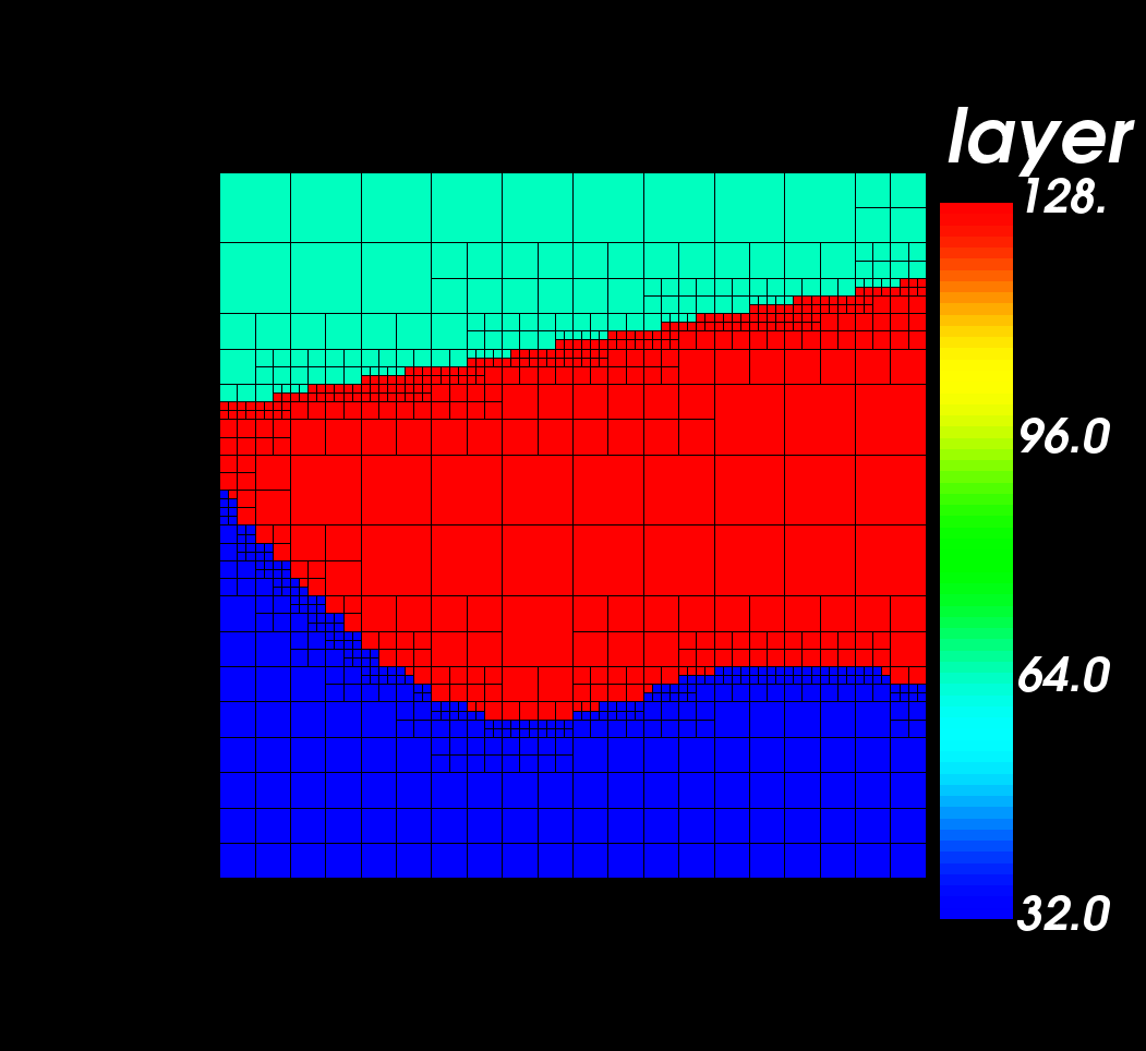
Figure 2: Auto-generated mesh for a soil domain with three non-horizontal non-planar soil layers.
Material models
To model the mechanical behavior of a material, three components need to be defined at every point in space and time - strain, elasticity tensor, stress.
Strain: Strain is a normalized measure of the deformation experienced by a material. In a 1-D scenario, say a truss is stretched along its axis, the axial strain is the elongation of the truss normalized by the length of the truss. In a 3D scenario, the strain is 3x3 tensor and there are three different ways to calculate strains from displacements - small linearized total strain, small linearized incremental strain, and finite incremental strain. Details about these methods can be found in Solid Mechanics Module.
Elasticity Tensor: The elasticity tensor is a 4th order tensor with a maximum of 81 independent constants. For MASTODON applications, the soil and structure are usually assumed to behave isotropically, i.e., the material behaves the same in all directions. Under this assumption, the number of independent elastic constants reduces from 81 to 2. The two independent constants that are usually provided for the soil are the shear modulus and Poissons's ratio, and for the structure it is the Young's modulus and Poisson's ratio.
Stress: The stress at a point in space and time is a 3x3 tensor which is a function of the strain at that location. The function that relates the stress tensor to the strain tensor is the constitutive model. Depending on the constitutive model, the material can behave elastically or plastically with an increment in strain.
Linear elastic constitutive model
In scenarios where the material exhibits a linear relation between stress and strain, and does not retain any residual strain after unloading, is called a linear elastic material. In linear elasticity, the stress tensor () is calculated as , where is the elasticity tensor, and is the strain tensor. This material model is currently used for numerically modeling the behavior of concrete and other materials used for designing a structure in MASTODON.
Nonlinear hysteretic constitutive model for soils (I-soil)
I-soil (Numanoglu (2017)) is a three dimensional, physically motivated, piecewise linearized nonlinear hysteretic material model for soils. The model can be represented by shear type parallel-series distributed nested components (springs and sliders) in one dimensional shear stress space and its framework is analogous to the distributed element modeling concept developed by Iwan (1967). The model behavior is obtained by superimposing the stress-strain response of nested components. Three dimensional generalization follows Chiang and Beck (1994) and uses von Mises (independent of effective mean stress) and/or Drucker-Prager (effective mean stress dependent) type shear yield surfaces depending on user's choice. The yield surfaces are invariant in the stress space Figure 3 . Thus, the model does not require kinematic hardening rule to model un/reloading stress-strain response and preserves mathematical simplicity.
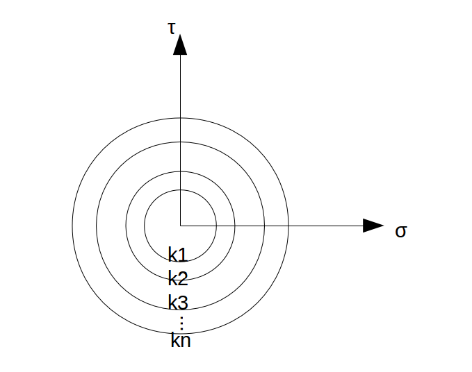
Figure 3: Invariant yield surfaces of the individual elastic-perfectly curves (after Chiang and Beck, 1994).
The current version of I-soil implemented in MASTODON utilizes Masing type un/reloading behavior and is analogous to MAT79 (LS-DYNA) material model but does not exhibit numerical instability observed in MAT79 (Numanoglu et al. (2017)). Masing type un/reloading is inherently achieved by the model because upon un/reloading the yielded nested components regain stiffness and strength. The cyclic response obtained from current version of the model is presented in Figure 4. Reduction factor type modification on un/reloading behavior (Phillips and Hashash (2009); Numanoglu et al. (2017)) is an ongoing study within MASTODON framework.
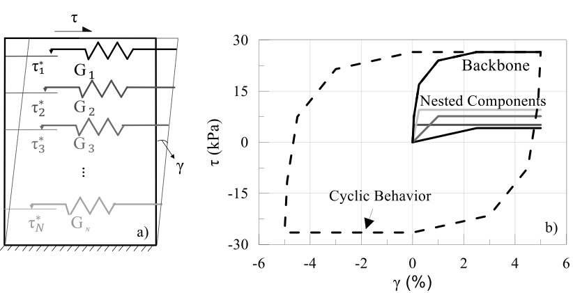
Figure 4: I-soil model details: (a) 1D representation by springs; (b) example monotonic and cyclic behavior of four nested component model (reprinted from Baltaji et al., 2017).
Main input for the current version of I-soil in MASTODON is a backbone curve at a given reference pressure. MASTODON provides variety of options to built backbone curve for a given soil type and reference pressure using following methods :
User-defined backbone curve (soil\_type = 'user_defined'): The backbone curve can be provided in a .csv file where the first column is shear strain points and the second column is shear stress points. The number of nested components that will be generated from this backbone curve depends on the number of discrete shear strain - shear stress pairs defined in the .csv file. When layered soil profile is present, .csv file for each reference pressure can be provided to the corresponding elements in the mesh.
Darendeli backbone curve (soil\_type = 'darandeli'): The backbone curve can be auto-generated based on empirical relations obtained from laboratory tests. Darendeli (2001) presents a functional form for normalized modulus reduction curves obtained from resonant column - torsional shear test for variety of soils. MASTODON utilizes this study and auto-generates the backbone shear stress - strain curves. The inputs for this option are (1) small strain shear modulus, (2) bulk modulus, (3) plasticity index, (4) overconsolidation ratio, (5) reference effective mean stress () at which the backbone is constructed, and (6) number of shear stress - shear strain points preferred by user to construct piecewise linear backbone curve. All the other parameters except the number of shear stress - shear strain points can be provided as a vector for each soil layer.
Darendeli (2001) study extrapolates the normalized modulus reduction curves after 0.1% shear strains. This extrapolation causes significant over/under estimation of the shear strength implied at large strains for different type of soils at different reference effective mean stresses (Hashash et al., 2010). Thus user should be cautious about implied shear strength when utilizing this option.
General Quadratic/Hyperbolic (GQ/H) backbone curve (soil\_type = 'gqh'): Darendeli (2001) study presented in previous item constructs the shear stress - shear strain curves based on experimentally obtained data. At small strains, the data is obtained using resonant column test, and towards the moderate shear strain levels, torsional shear test results are used. Large strain data are extrapolation of the small to medium shear strain data. This extrapolation underestimates or overestimates the shear strength mobilized at large shear strains. Therefore, implied shear strength correction is necessary to account for the correct shear strength at large strains. GQ/H constitutive model proposed by Groholski et al. (2016) has a unique curve fitting scheme embedded into the constitutive model that accounts for mobilized strength at large shear strains by controlling the shear strength. This model uses taumax, theta\_1 through 5, small strain shear modulus, bulk modulus and number of shear stress - shear strain points preferred by user to construct piecewise linear backbone curve. The parameter taumax is the maximum shear strength that can be mobilized by the soil at large strains. The parameters theta\_1 through 5 are the curve fitting parameters and can be obtained using DEEPSOIL (Hashash et al., 2016). Other than the number of points, all the other parameters can be given as a vector for the different soil layers. The number of points, which determines the number of elastic-perfectly plastic curves to be generated, is constant for all soil layers.
Once the backbone curve is provided to I-soil, the model determines the properties for nested components presented in Figure 4. The stress integration for each nested component follows classic elastic predictor - plastic corrector type radial return algorithm (Simo and Hughes (2006)) and model stress is obtained by summing the stresses from each nested component:
where is the total shear stress, is the shear modulus of the nested component, is the shear strain, is the yield stress of the nested component, and represents the number of components that have not yet yielded out of the total nested components.
Small strain shear modulus can be varied with effective mean stress via:
where, is the initial shear modulus, is the tension pressure cut off and is mean effective stress dependency parameter obtained from experiments. The shear modulus reduces to zero for any mean effective stress lower than to model the failure of soil in tension. Note that the mean effective stress is positive for compressive loading. Thus, should be inputted as negative.
Yield criteria of the material can also be varied with effective mean stress dependent behavior as:
where, , and are parameters that define how the yield stress varies with pressure.
Lead-Rubber Isolator
Lead-rubber (LR) seismic isolators are composed of alternating layers of natural rubber and steel shims with steel flange plates at top and bottom, and a central cylindrical lead core. Continuum modeling of LR bearings is computationally expensive and impractical for applications involving large structures with tens to hundreds of isolators. Hence, the two-node model developed by Kumar et al. (2015) is adopted here. The isolator model has six degrees of freedom (3 translations and 3 rotations) at each node and is capable of simulating nonlinear behavior in both axial and shear directions. The physical model of the two-node isolator element is shown in Figure 5 below. For a detailed description on the implementation of numerical model, refer to (Kumar et al., 2015).
.](../../media/materials/lr_isolator/physicalmodel.png)
Figure 5: Discrete, two-noded model of an LR bearing: (a) degrees of freedom, and (b) discrete spring representation (Kumar et al., 2014).
This model captures the following physical behaviors:
Axial
Buckling in compression
Buckling load variation with shear deformation
Cavitation and post-cavitation behavior in tension
Shear
Viscoelastic behavior of rubber
Hysteretic behavior of the lead core
Strength degradation due to the heating of the lead core
Coupling in axial and shear
Shear stiffness variation with axial load
Axial stiffness variation with shear deformation
Axial (local X direction)
Compression
The composite action of the rubber and the steel shims result in high axial stiffness of a bearing. The expression for the critical buckling load in compression is derived from the two-spring model proposed by Koh and Kelly (1987) as shown in Eq. (5).
(5)
where,
Eq. (5) provides the critical buckling load at zero shear displacement. Experimental investigations have shown that the critical buckling load is a function of the shear deformation. Warn and Whittaker (2006) proposed a simplified expression for the critical buckling load as a function of the overlap bonded rubber area. The critical buckling load is updated at every analysis step based on the current shear deformation in the bearing.
(6)
where,
is the rotational modulus
is the height of isolator excluding the end plates
is the total rubber thickness
is the shear modulus of the rubber
is the initial bonded rubber area
is the current value of the critical buckling load
is the critical buckling load at zero shear displacement
is the current overlap area of bonded rubber
Once the bearing buckles, the axial stiffness is reduced to zero. However, to avoid numerical problems, a very small value of axial stiffness is assigned to the post-buckling region.
Tension
Beyond a certain tensile stress, rubber undergoes cavitation, which is an expansion of existing voids or defects in the material. Cavitation results in an inelastic deformation due to the onset of permanent damage. The LR isolator exhibits linear elastic behavior, till the point of cavitation (,), where, and are the deformation and force, respectively, at the onset of cavitation. Due to the breakage of rubber-filler bonds, the post-cavitation stiffness is reduced. Constantinou et al. (2007) suggested an expression for post-cavitation stiffness as:
(7)
Integrating the Eq. (7), the expression for the post-cavitation tensile force is obtained as:
(8)
where,
is the initial cavitation force
is a cavitation parameter
is the initial cavitation deformation
is the tensile deformation
is Young's modulus of the rubber
When the bearing is loaded beyond the point of cavitation and unloaded, it does not unload with the initial elastic stiffness. The unloading stiffness is smaller than the elastic stiffness because of formation of cavities in the rubber. The cavitation strength is a function of a damage parameter which varies from zero to one. At maximum damage, the tensile strength of rubber layers is not completely zero. Therefore an upper bound of 0.75 value is assumed for the damage parameter.
(9)
where,
is the damage constant
is the current value of the damage parameter
is the upper bound on the damage parameter
For (namely, at the cavitation point), is equal to 0 implying no damage. As the tensile deformation increases, the damage parameter converges to . The reduced cavitation strength as a function of damage parameter is calculated as
(10)
Figure 6 shows the assumed response of a LR isolator to cyclic axial loading (both compression and tension).
.](../../media/materials/lr_isolator/axialformulation.png)
Figure 6: Axial response of an elastomeric isolator (Kumar et al., 2014).
where,
is the axial stiffness of the isolator
is the current shear deformation
is the radius of gyration of the isolator
Shear behavior (local Y and Z directions)
The smoothed hysteric model proposed by Park et al. (1986) and extended by Nagarajaiah et al. (1989) is used to model the behavior of a lead-rubber bearing in shear. The shear resistance of the LR bearing is a combination of the viscoelastic behavior of the rubber layers and the hysteretic behavior of the lead core, as shown in Figure 7. The behavior of rubber is characterized by elastic stiffness, viscous damping terms and the nonlinear hysteretic contribution of the lead core is modeled using a Bouc-Wen formulation.
.](../../media/materials/lr_isolator/shearformulation.png)
Figure 7: Shear behavior of the LR isolator (Kumar et al., 2015).
(11)
where,
subscripts and correspond to shear 1 (local Y) and shear 2 (local Z) directions respectively, as shown in Figure 5
is the viscous damping co-efficient of the rubber</br> is the shear stiffness of the rubber material </br> is the dynamic yield strength of the lead core </br> is the cross sectional area of the lead core
The Bouc-Wen formulation introduces two hysteresis evolution parameters, and , which are functions of the shear displacements and , in the local Y and Z directions respectively.
(12)
where,
(13)
Eq. (12) is iteratively solved using the Newton-Raphson method to calculate the values of and at every analysis step in MASTODON.
Lead core heating
When the LR isolator is subjected to cyclic loads in shear, the temperature of the lead core increases. The effective yield stress of the lead core used in Eq. (11) varies with the temperature of the lead core, which is a function of time. Therefore, at every time step, the temperature of lead core is calculated and the dynamic yield strength of the lead is adjusted. The relationship between the dynamic yield strength of the lead core and the instantaneous temperature was proposed by Kalpakidis and Constantinou (2009a) as
(14)
where,
is the dynamic strength of lead core at the current temperature
is the dynamic yield strength of lead core at a reference temperature
is the instantaneous temperature of the lead core
Coupled shear and axial response
When the axial load on the bearing is close to the critical buckling load, the shear stiffness of the rubber is reduced substantially. This reduction in shear stiffness as a function of axial load is approximated using the equation from Kelly (1993).
(15)
where,
P is the current axial load on the isolator
The axial stiffness of the LR isolator is also a function of the overlap bonded rubber area, which is a function of the shear deformation. A simplified expression formulated by Koh and Kelly (1987) and Warn et al. (2007) is adopted here (16)
where,
is the current shear deformation
Limitations
Currently, this formulation is limited to simulations that result in small rigid-body rotations in the isolator because the isolator deformations are transformed from the global to the local coordinate system using a transformation matrix that is calculated from the initial position of the isolator. This transformation matrix is not updated during the analysis because, seismic isolators typically undergo very small rigid-body rotations.
The post-buckling behavior of the LR isolator is modeled using a very small axial stiffness () of the initial stiffness to avoid numerical convergence problems.
The mass of the LR bearing is not modeled. The user can model the mass of an isolator using inertial NodalKernels as shown in a seismic simulation example here.
Friction PendulumTM Isolator
Friction PendulumTM (FP) bearings are used to seismically isolate structures, including critical facilities such as nuclear power plants. The single concave FP bearing consists of a spherical sliding surface, a slider coated with PTFE-type composite material, and a housing plate. Figure 15 and Figure 16 shows components and part sectional view of a single concave Friction PendulumTM bearing, respectively.
](../../media/materials/fp_isolator/fp_components.png)
Figure 15: Components of a single Friction PendulumTM bearing ((EPS), 2012)
](../../media/materials/fp_isolator/fp_sectionalview.png)
Figure 16: Sectional view of a single concave Friction PendulumTM bearing (Kumar et al., 2015b)
Continuum modeling of FP bearings is computationally expensive and impractical for applications involving structures with tens to hundreds of bearings. Hence a two-node model developed by Kumar et al. (2015b) is adopted here. The bottom node represents the concave sliding surface, and the top node represents the articulated slider. The two-node model has six degrees of freedom (3 translations and 3 rotations), at each node and is capable of simulating nonlinear hysteric behavior in the FP bearing. The physical model and spring representation of the two-node FP isolator element is similar to that of the lead-rubber isolator as shown in fig.
Force-displacement relationship
Friction PendulumTM bearings dissipate the energy induced during an earthquake through nonlinear hysteretic behavior in shear. The lateral force-displacement relationship of a single concave FP bearing is characterized by two parameters: yield strength and post elastic stiffness, and can be represented by the bi-linear curve of Figure 8.
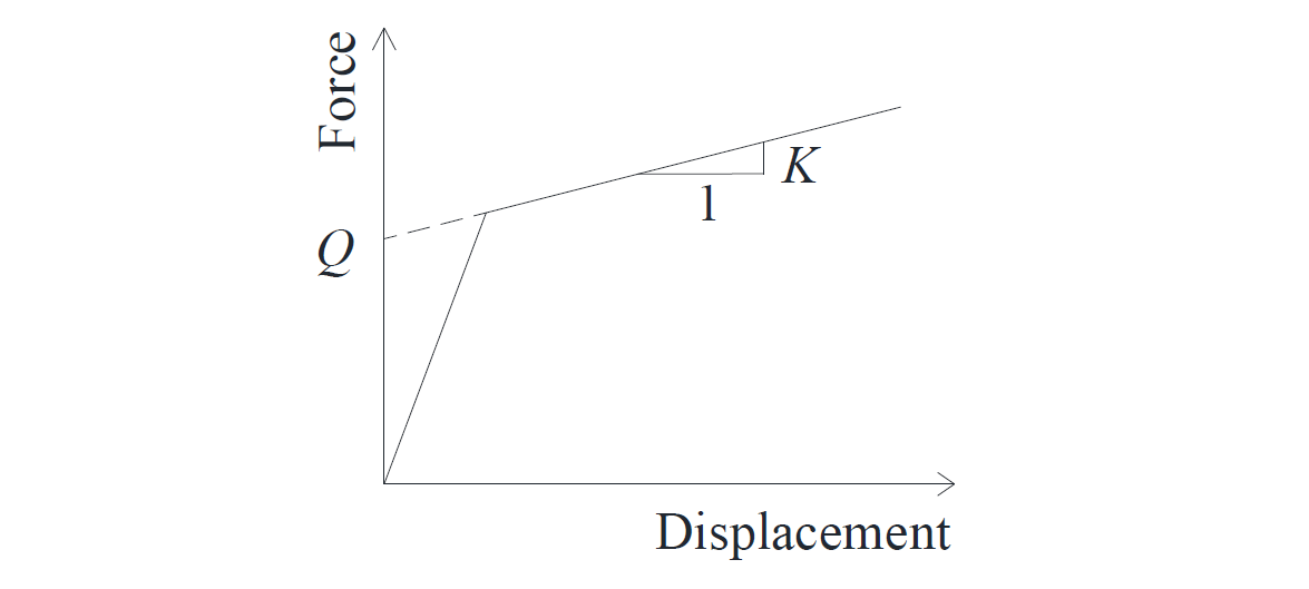
Figure 8: Lateral force-displacement relationship of a single concave FP bearing
The yield strength and the post-elastic stiffness can be calculated as,
(17)
(18)
where,
is the yield strength
is the post elastic stiffness
is the instantaneous axial load, and
is the effective radius of curvature of the sliding surface.
Parameters and depends on the coefficient of sliding friction and the axial load on the bearing. For detailed information on the numerical implementation of the nonlinear hysteretic behavior of the FP bearing in shear, refer to Kumar et al. (2015) (page:106-107). Additionally, the FP bearing exhibits very large stiffness in axial, torsional and rotational directions and is therefore modeled as a linear elastic material with large stiffness in these degrees-of-freedom.
Coefficient of sliding friction
The lateral force-displacement relationship of the FP bearing is governed by the coefficient of sliding friction. At a given instant of time the coefficient of sliding friction depends on the instantaneous sliding velocity, instantaneous axial pressure, and the temperature of the sliding interface.
(19)
where,
is the coefficient of sliding friction at given time
is the instantaneous sliding velocity
is the instantaneous axial pressure, and
is the instantaneous temperature of the sliding surface.
Kumar et al. (2015b) developed a framework to account for the variation in due to the combined effect of velocity, pressure, and temperature and it is adopted here. The sliding velocity and the axial pressure on the bearing are governed by the response of the superstructure. The temperature at the sliding surface is a function of the coefficient of friction, sliding velocity, instantaneous axial pressure and, thermal and heat flux parameters of the material (typically stainless steel):
(20)
where,
k is the thermal conductivity of the sliding interface material, and
D is the thermal diffusivity of the sliding interface material.
It is evident from Eq. (19) and Eq. (20), that and are interdependent. This complex interdependence of the coefficient of sliding friction, sliding velocity, instantaneous axial pressure, and the temperature at the sliding surface is described using the flowchart of Figure 9.
.](../../media/materials/fp_isolator/fp_interdependence.png)
Figure 9: Interdependence of parameters governing the lateral force-displacement relationship of a FP bearing (Kumar et al., 2015b).
Dependence of the coefficient of friction on the sliding velocity
Mokha et al. (1988) proposed an expression to account for the dependence of the coefficient of friction on the instantaneous sliding velocity as
(21)
where,
is the friction coefficient at a very small sliding velocity
is the friction coefficient at a very high sliding velocity, and
is a rate parameter.
Based on the experimental data, the ratio is assumed to be a constant value of 0.5 (Kumar et al., 2015b). The modified expression for coefficient of friction as a function of instantaneous sliding velocity, at constant axial load and temperature, can be written as:
(22)
Dependence of the coefficient of friction on the axial pressure
Kumar et al. (2015b) proposed an expression for the coefficient of sliding friction as a function of axial pressure at very high sliding velocity, and is given by
(23)
where,
is the reference axial pressure
is the co-efficent of sliding friction when the axial pressure on the bearing () is equal to the reference pressure (), and
and are constants.
The assumption of for all values of axial pressure allows the coefficient of sliding friction to be expressed as the product of the coefficient of friction measured at a reference pressure and a term that depends on the instantaneous axial pressure. Based on the experiments, and can be set equal to 0.7 and 0.02 respectively (Kumar et al., 2015b). Rewriting the expression for as a function of :
(24)
Dependence of the coefficient of friction on the temperature at sliding interface
The coefficient of sliding friction decreases as the number of cycles of loading increase. Kumar et al. (2015b) proposed an expression to define the coefficient of friction as a function of the instantaneous temperature, at a reference axial pressure and very high sliding velocity as
(25)
where,
is the coefficient of friction at a temperature
is the coefficient of friction measured at the reference temperature , and
is the instantaneous temperature.
During the analysis, it is difficult to monitor the temperature over the entire sliding surface. To address the heating, Kumar et al. (2015b) proposed an alternate approach namely, to monitor the temperature at the center of sliding surface only. When the slider is above the center of sliding surface, the temperature increases, and drops as the slider moves away. This increase in temperature at the monitoring location is governed by the heat flux parameters and the path of the slider, and is given by Eq. (26)
(26)
where,
is the increase in temperature
is the depth measured from the sliding surface,
is the thermal diffusivity of the sliding interface material,
is the thermal conductivity of the sliding interface material, and
is the heat flux.
At a given instant of time, the instantaneous heat flux, at the monitoring location can be expressed as
(27)
Dependence of the coefficient of friction on the combined effects of temperature, axial pressure and sliding velocity
During an earthquake, the sliding velocity, axial pressure and the temperature at the sliding surface of a FP bearing changes continuously. The combined effect of all the three has to be considered to determine the coefficient of sliding friction. From Eq. (22), Eq. (24),and Eq. (25), the factors accounting for friction dependence on the velocity, pressure, and the temperature () can be written as
(28)
(29)
(30)
The coefficient of sliding friction as a function of the instantaneous sliding velocity, axial pressure on the bearing and the temperature at the center of the sliding surface is updated as:
(31)
where,
is the factor accounting for friction dependence on the sliding velocity
is the factor accounting for friction dependence on the axial pressure on the bearing
is the factor accounting for friction dependence on the temperature at center of the sliding surface, and
is the coefficient of sliding friction at refernce pressure , measured at high velocity of sliding with the temperature at the center of the sliding surface being .
Nonlinear Fluid Viscous Damper
ComputeFVDamperElasticity material is used to simulate the hysteretic response of a nonlinear FVD element in MASTODON. Nonlinear fluid viscous dampers (FVDs) are seismic protective devices used to mitigate the effects of intense earthquake shaking on engineered structures such as nuclear power plants. Fluid viscous dampers operate on the principle of fluid flow through the orifice creating a differential pressure across the piston head and develops an internal resisting force in the damper. Reinhorn et al. (1995) proposed a simplified expression for the force in the damper as a function of the fractional power of relative velocity as shown in Eq. (32)
(32)
where, is the damping coefficient, is the velocity exponent, and is the instantaneous relative velocity in the damper.
The response of the FVD is characterized by two parameters, , and . For = 1, Eq. (32) models a linear damper and the typical range for is between 0.3 and 1.0 for seismic applications. Fluid viscous dampers are typically installed in the structure with an in-line brace, which provides stiffness to the damper assembly. Reinhorn et al. (1995) observed that such stiffness had to be addressed for response calculations and therefore modeled explicitly. The brace can be modeled as a spring in series with the nonlinear dashpot, and the combined behavior of spring and dashpot is best represented using the Maxwell formulation, as shown in Figure 10.
.](../../media/materials/fv_damper/fv_maxwellmodel.png)
Figure 10: Mathematical model for a nonlinear FVD element (Akcelyan et al., 2018).
The Maxwell model of Figure 10 also includes the flexibility of the gussets, brackets and clevises. The overall stiffness of the damper assembly is calculated as
(33)
In the Maxwell model, the nonlinear dashpot and the spring are in series and therefore the force in the dashpot and spring are equal. This force is given by,
(34)
and the expressions for the total displacement and the total velocity of the damper are
(35)
(36)
where, and are the relative displacement and the relative velocity in the spring, and and are the relative displacement and the relative velocity in the dashpot.
From Eq. (34), the rate of change of force can be written as
(37)
Using Eq. (35) & Eq. (36), and rewriting the expression for the rate of change of force
(38)
Eq. (38) is a first-order differential equation in the form of an initial value problem (IVP)
(39)
Dormand and Prince (1980) proposed an iterative integration scheme known as Dormand Prince (DP54), to solve a generalized initial value problem of the form shown in Eq. (39) above. Iterative algorithms such as DP54 are computationally more efficient than traditional integration schemes for numerical solution of initial value problems. Akcelyan et al. (2018) proposed a framework to obtain the numerical solution of nonlinear FVD based on DP54 algorithm and that has been adopted here. For detailed information on the numerical implementation, specific to the FVD element, refer to Akcelyan et al. (2018).
Foundation-soil interface models
The foundation-soil interface is an important aspect of NLSSI modeling. The foundation-soil interface simulates geometric nonlinearities in the soil-structure system: gapping (opening and closing of gaps between the soil and the foundation), sliding, and uplift.
Thin-layer method
An efficient approach to modeling the foundation-soil interface is to create a thin layer of the I-Soil material at the interface, as illustrated in Figure 11 below.
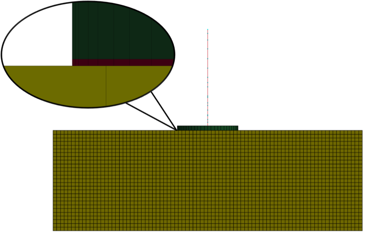
Figure 11: Modeling the foundation-soil interface as a thin layer for a sample surface foundation.
The red layer between the foundation (green) and soil (yellow) is the thin layer of I-Soil. The properties of this thin layer are then adjusted to simulate Coulomb friction between the surfaces. The Coulomb-friction-type behavior can be achieved by modeling the material of the thin soil layer as follows:
Define an I-Soil material with a user-defined stress-strain curve.
Calculate the shear strength of the thin layer as , where is the shear strength, is the friction coefficient, and is the normal stress on the contact surface. The shear strength of the thin layer is the stress at which sliding starts at the interface. Therefore, this shear strength should be proportional to the normal stress to simulate Coulomb friction. This can be achieved by setting the initial shear strength equal to the reference pressure, . The reference pressure can then be set to an arbitrary positive value, such as the average normal stress at the interface from gravity loads. The shear strength will then follow the equation
Define the stress-strain curve to be almost elastic-perfectly-plastic, and such that the shear modulus of the thin layer is equal to the shear modulus of the surrounding soil, in case of an embedded foundation. If the foundation is resting on the surface such as in Figure 11 above, the shear modulus of the thin layer soil should be as high as possible, such that the linear horizontal foundation stiffness is not reduced due to the presence of the thin layer. A sample stress-strain curve is shown in Figure 12 below. The sample curve in the figure shows an almost bilinear shear behavior with gradual yielding and strain hardening, both of which, are provided to reduce possible high-frequency response. High-frequency response is likely to occur if a pure Coulomb friction model (elastic-perfectly-plastic shear behavior at the interface) is employed, due to the sudden change in the interface shear stiffness to zero.
Figure 12: Sample shear-stress shear-strain curve for modeling the thin-layer interface using I-Soil.
Turn on pressure dependency of the soil stress-strain curve and set , and to 0, 0 and 1, respectively. This ensures that the stress-strain curve scales linearly with the normal pressure on the interface, thereby also increasing the shear strength in the above equation linearly with the normal pressure, similar to Coulomb friction.
Use a large value for the Poisson's ratio, in order to avoid sudden changes in the volume of the thin-layer elements after the yield point is reached. A suitable value for the Poisson's ratio can be calculated by trial and error.
Following the above steps should enable the user to reasonably simulate geometric nonlinearities. These steps will be automated in MASTODON in the near future.
Boundary Conditions
Non-reflecting boundary
This boundary condition applies a Lysmer damper (Lysmer and Kuhlemeyer, 1969) on a given boundary to absorb the waves hitting the boundary. To understand Lysmer dampers, let us consider an uniform linear elastic soil column and say a 1D vertically propagating P wave is traveling through this soil column. Then the normal stress at any location in the soil column is given by:
(40)
where, is the Young's modulus, is the normal stress, is the normal strain, is the density, is the P-wave speed and is the particle velocity. Note that for a 3D problem, the P-wave speed is .
The stress in the above equation is directly proportional to the particle velocity which makes this boundary condition analogous to a viscous damper with damping coefficient of . So truncating the soil domain and placing this damper at the end of the domain is equivalent to simulating wave propagation in an infinite soil column provided the soil is made of linear elastic material and the wave is vertically incident on the boundary.
If the soil is not linear elastic or if the wave is incident at an angle on the boundary, the waves are not completely absorbed by the Lysmer damper. However, if the non-reflecting boundary is placed sufficiently far from the region of interest, any reflected waves will get damped out by Rayleigh damping or hysteretic material behavior before it reaches the region of interest.
Seismic force
In some cases, the ground excitation is measured at a rock outcrop (where rock is found at surface level and there is no soil above it). To apply this to a location where rock is say m deep and there is soil above it, a sideset is created at m depth and the ground excitation (converted into a stress) is applied at this depth. To apply ground excitation as a stress, the input function should be given as ground velocity.
To convert a velocity applied normal to the boundary into a normal stress, the normal stress equation above can be used. Using a similar argument as discussed in the section above, to convert a velocity applied tangential to the boundary into a shear stress, Equation Eq. (41) can be used.
(41) where, is the shear wave speed and is the shear stress.
Preset acceleration
If the ground excitation was measured at a depth within the soil by placing an accelerometer at that location, then it is termed as a within-soil input. This time history contains the wave that was generated by the earthquake (incoming wave) and the wave that is reflected off the free surface. This ground excitation time history is usually available in the form of a acceleration time history. Since MASTODON is a displacement controlled algorithm, i.e., displacements are the primary unknown variables, the acceleration time history is first converted to the corresponding displacement time history using Newmark time integration equation. This displacement time history is then prescribed to the boundary.
Earthquake fault rupture
The orientation of an earthquake fault is described using three directions - strike (), dip () and slip direction () as shown in Figure 13, which is courtesy of Aki and Richards (2012).
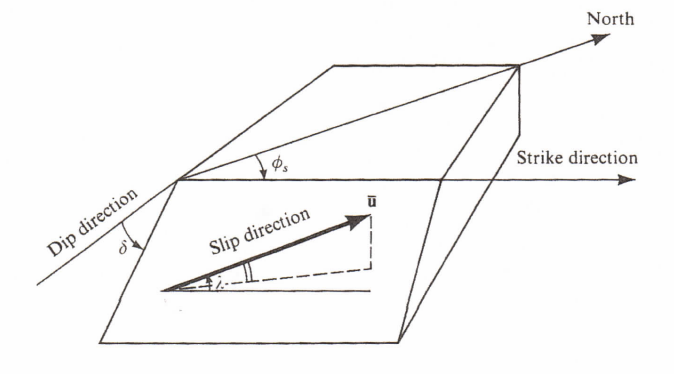
Figure 13: Definition of the fault-orientation parameters - strike , dip and slip direction . The slip direction is measured clockwise around from north, with the fault dipping down to the right of the strike direction. Strike direction is also measured from the north. is measured down from the horizontal.
In MASTODON, earthquake fault is modeled using a set of point sources. The seismic moment () of the earthquake point source in the fault specific coordinate system is:
where, is the shear modulus of the soil, is the area of fault rupture and is the spatially averaged slip rate of the fault.
When this seismic moment is converted into the global coordinate system (x, y and z) with the x direction oriented along the geographic north and z direction along the soil depth, the resulting moment can be written in a symmetric matrix form whose components are as follows:
Each component of the above matrix is a force couple with the first index representing the force direction and the second index representing the direction in which the forces are separated (see Figure 14; Aki and Richards (2012)).
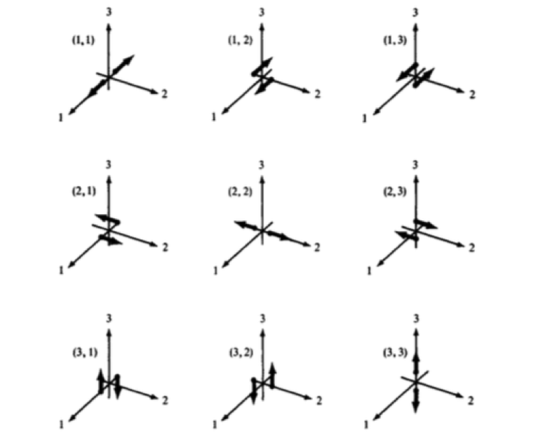
Figure 14: The nine different force couples required to model an earthquake source.
The total force in global coordinate direction resulting from an earthquake source applied at point in space is then:
where, is the delta function in space.
When many earthquake sources are placed on the earthquake fault, and they rupture at the same time instant, then an approximation to a plane wave is generated. If one of the point sources is specified as the epicenter and the rupture speed () is provided, then the other point sources start rupturing at , where is the distance between the epicenter and the other point source.
Outputs
This section presents some of the common post-processing tools available in MASTODON that help in understanding the wave propagation, and response of structures and soils to earthquake excitation.
Response histories
In MASTODON, the time history of any nodal variable (displacement, velocity, acceleration) or elemental variable (stress, strain) can be requested as output. The nodal variable time histories can be requested at a set of nodes and this can help in visualizing the wave propagation.
Response spectra
An important quantity that is used in understanding the response of a structure is the velocity/acceleration response spectra. This contains information about the frequency content of the velocity/acceleration at a particular location. The velocity/acceleration response spectra at a frequency is obtained by exciting a single degree of freedom (SDOF) system with natural frequency of with the velocity/acceleration time history recorded at that location, and obtaining the peak velocity/acceleration experienced by the SDOF. This exercise is repeated for multiple frequencies to obtain the full response spectra.
Housner spectrum intensity
The response spectra is very useful for understanding the response of the system at one location. However, if the response at multiple locations have to be compared, a single value that can summarize the response at a location is much more useful. Housner spectrum intensity is the integral of the velocity response spectra between 0.25-2.5 s (or 0.4-4 Hz). This packs the information from the velocity response spectra at multiple frequencies into a single value and reasonably represents the response at a location.
Response history mean
In MASTODON, the mean response history given the response histories of the same type (i.e., displacements, velocities, or accelerations) at a list of nodes or a boundary can be requested as an output. The mean response history can help understanding how intense the response is, in an average sense, at a certain depth in the soil, or at the foundation, or at a certain height of the nuclear power plant, etc.
References
- Earthquake Protection Systems (EPS).
http://www.earthquakeprotection.com/single_pendulum_bearing.html, 2012.[BibTeX]
- Sarven Akcelyan, Dimitrios G. Lignos, and Tsuyoshi Hikini.
Adaptive numerical method algorithms for nonlinear viscous and bilinear oil damper models subjected to dynamic loading.
Soil Dynamics and Earthquake Engineering, 113:488–502, 2018.[BibTeX]
- K. Aki and P. G. Richards.
Quantitative Seismology.
University Science Books; Second edition, 2012.[BibTeX]
- K. W. Campbell.
Estimates of shear-wave Q and $\kappa 0$ for unconsolidated and semiconsolidated sediments in eastern north america.
Bulletin of the Seismological Society of America, 99(4):2365–2392, 2009.[BibTeX]
- T. K. Caughey.
Classical normal-modes in damped linear dynamic systems.
Journal of Applied Mechanics, 27(2):269–271, 1960.[BibTeX]
- D. Y. Chiang and J. L. Beck.
A new class of distributed-element models for cyclic plasticity -i. theory and application.
International Journal of Solids and Structures, 31(4):469–484, 1994.[BibTeX]
- J. Coleman, C. Bolisetti, and A. Whittaker.
Time-domain soil-structure interaction analysis of nuclear facilities.
Nuclear engineering and design, 298:264–270, 2016.[BibTeX]
- M. C. Constantinou, A. S. Whittaker, Y. Kalpakidis, D. M. Fenz, and G. P. Warn.
Performance of seismic isolation hardware under service and seismic loading.
Technical Report MCEER-07-0012, Multidisciplinary Center for Earthquake Engineering Research, Buffalo, New York, 2007.[BibTeX]
- M. B. Darendeli.
Development of a new family of normalized modulus reduction and material damping curves.
PhD dissertation, University of Texas at Austin, 2001.[BibTeX]
- J. R. Dormand and P. J. Prince.
A family of embedded runge-kutta formulae.
Journal of Computational and Applied Mathematics, 6(1):19–26, 1980.[BibTeX]
- D. Groholski, Y. Hashash, B. Kim, M. Musgrove, J. Harmon, and J. Stewart.
Simplified model for small-strain nonlinearity and strength in 1d seismic site response analysis.
Journal of Geotechnical and Geoenvironmental Engineering, 2016.[BibTeX]
- Y. Hashash, M. Musgrove, J. Harmon, D. Groholski, C. Phillips, and D. Park.
Deepsoil v6.1, user manual.
Urbana, IL, Board of Trustees of University of Illinois at Urbana-Champaign, 2016.[BibTeX]
- Y. M. A. Hashash, C. Phillips, and D. Groholski.
Recent advances in non-linear site response analysis.
Fifth International Conference on Recent Advances in Geotechnical Earthquake Engineering and Soil Dynamics, San Diego, 2010.[BibTeX]
- W. Iwan.
On a class of models for the yielding behavior of continuous and composite systems.
Journal of Applied Mechanics, ASME, 34(E3):612–617, 1967.[BibTeX]
- I. V. Kalpakidis and M. C. Constantinou.
Effects of heating on the behavior of lead-rubber bearings i:theory.
Journal of Structural Engineering, 135(12):1450–1461, 2009a.[BibTeX]
- J. M. Kelly.
Earthquake-resistant design with rubber.
Springer-Verlag, London, 1993.[BibTeX]
- C. G. Koh and J. M. Kelly.
Effects of axial load on elastomeric isolation bearings.
Technical Report EERC/UBC-86/12, Earthquake Engineering Research Center, University of California, Berkeley, CA, 1987.[BibTeX]
- M Kumar, A.S Whittaker, and M.C Constantinou.
Seismic isolation of nuclear power plants using sliding bearings.
Technical Report MCEER-15-0006, Multidisciplinary Center for Earthquake Engineering Research, Buffalo, New York, 2015b.[BibTeX]
- M. Kumar, A. S. Whittaker, and M. C. Constantinou.
An advanced numerical model of elastomeric seismic isolation bearings.
Earthquake Engineering and Structural Dynamics, 43(13):1995–1974, 2014.[BibTeX]
- M. Kumar, A. S. Whittaker, and M. C. Constantinou.
Seismic isolation of nuclear power plants using elastomeric bearings.
Technical Report MCEER-15-0008, Multidisciplinary Center for Earthquake Engineering Research, Buffalo, New York, 2015.[BibTeX]
- A. O. L. Kwok, J. P. Stewart, Y. M. A. Hashash, N. Matasovic, R. Pyke, Z. Wang, and Z. Yang.
Use of exact solutions of wave propagation problems to guide implementation of nonlinear, time-domain ground response analysis routines.
ASCE Journal of Geotechnical and Geoenvironmental Engineering, pages 1385–1398, 2007.[BibTeX]
- J. Lysmer and R. L. Kuhlemeyer.
Finite dynamic model for infinite media.
Journal of the Engineering Mechanics Division, 95(4):859–878, 1969.[BibTeX]
- G. Marmureanu, D. Bratosin, and C. O. Cioflan.
The dependence of Q with seismic-induced strains and frequencies for surface layers from resonant columns.
Seismic Hazard of the Circum-Pannonian Region, pages 269–279, 2000.[BibTeX]
- F. Y. Menq.
Dynamic properties of sandy and gravelly soils.
PhD dissertation, University of Texas at Austin, 2003.[BibTeX]
- A Mokha, Constantinou. M. C, and Reinhorn. A. M.
Teflon bearings in aseismic base isolation: experimental studies and mathematical modeling.
Technical Report NCEER-88-0038, National Center for Earthquake Engineering Research, Buffalo, New York, 1988.[BibTeX]
- S. Nagarajaiah, A. M. Reinhorn, and M. C. Constantinou.
Nonlinear dynamic analysis of three-dimensional base isolated structures (3d-basis).
Technical Report NCEER-89-0019, National Center for Earthquake Engineering Research, Buffalo, New York, 1989.[BibTeX]
- N. M. Newmark.
A method of computation for structural dynamics.
Journal of Engineering Mechanics, 85(EM3):67–94, 1959.[BibTeX]
- O. A. Numanoglu.
Phd in progress.
University of Illinois at Urbana-Champaign, 2017.[BibTeX]
- O. A. Numanoglu, Y. M. A. Hashash, A. Cerna-Diaz, S. M. Olson, L. Bhaumik, and C. J. Rutherford.
Nonlinear 3-d modeling of dense sand and the simulation of a soil-structure system under multi-directional loading.
Geotechnical Frontiers 2017, pages 379–388, 2017.[BibTeX]
- O. A. Numanoglu, M. M. Musgrove, J. A. Harmon, and Y. M. A. Hashash.
Generalized non-masing hysteresis model for cyclic loading.
Manuscript submitted for puplication, 2017.[BibTeX]
- Y. J. Park, Y. K. Wen, and A. H. S Ang.
Random vibrations of hysteretic systems under bi-directional ground motions.
Earthquake Engineering and Structural Dynamics, 14(4):543–557, 1986.[BibTeX]
- C. Phillips and Y. M. A. Hashash.
Damping formulation for nonlinear 1d site response analyses.
Soil Dynamics and Earthquake Engineering, 29(7):1143–1158, 2009.[BibTeX]
- D. C. F. Lo Presti, O. Pallara, and A. Cavallaro.
Damping ratio of soils from laboratory and in-situ tests.
Proc. 14th Int. Conf. Soil Mech. Found. Engng, pages 391–400, 1997.[BibTeX]
- A. M. Reinhorn, C. Li, and M. C. Constantinou.
Experimental and analytical investigation of seismic retrofit of structures with supplemental damping, part 1: fluid viscous damping devices.
Technical Report NCEER-95-0001, National Center for Earthquake Engineering Research, Buffalo, New York, 1995.[BibTeX]
- S. Shibuya, T. Mitachi, F. Fukuda, and T. Degoshi.
Strain rate effects on shear modulus and damping of normally consolidated clay.
pages 365–375, 1995.[BibTeX]
- J. C. Simo and T. J. R. Hughes.
Computational inelasticity.
Springer Science and Business Media, 2006.[BibTeX]
- G. P. Warn and A. S. Whittaker.
A study of coupled horizontal-vertical behavior of elastomeric and lead-rubber seismic isolation bearings.
Technical Report MCEER-06-0011, Multidisciplinary Center for Earthquake Engineering Research, Buffalo, New York, 2006.[BibTeX]
- G. P. Warn, A. S. Whittaker, and M. C. Constantinou.
Vertical stiffness of elastomeric and lead-rubber seismic isolation bearings.
Journal of Structural Engineering, 133(9):1227–1236, 2007.[BibTeX]
- K. B. Withers, K. B. Olsen, and S. M. Day.
Memory-efficient simulation of frequency-dependent q.
Bulletin of the Seismological Society of America, 105(6):3129–3142, 2015.[BibTeX]