Tutorial
This tutorial is a breakdown of a full MASTODON input file. It will begin as a very simple site response analysis and will gain complexity as the tutorial proceeds. We will step through the problem in the same sort of way that an advanced user would. Each part of the input file will be briefly explained and links to useful areas in the documentation site will be provided.
Linear Site Response
The first step is to begin with something very simple. Linear site response. No gravity, linear soil, everything in this step should be fairly straightforward.
In general, users do not just start writing a text input file from scratch, instead the user should find a test or example input file that is generally related to the problem being set up and modify that input to better fit his or her model. With that stated, feel free to use this input file as a skeleton for your future site response analysis models. This tutorial will step through each block of text that comprises this input file.
The order in which you define these blocks within the input file does not matter! There is somewhat of a natural progression when it comes to defining the various blocks, but the order is not significant.
The Model
The model we will be stepping through in this tutorial is a 1D site response. The model is a 100 m soil column containing 100 elements, each measuring 1 m x 1 m x 1 m. The base of the soil column is prescribed the acceleration history shown in Figure 1. Note that this is just a contrived example problem, there is no significance or meaning associated with the input motion. The outputs include an exodus file that can be used for visualizing results, and csv files containing accelerations and response spectra calculations at the top of the column. These outputs will be discussed in detail further into the tutorial. The input file is 'site_reponse_1.i' It can be executed in MASTODON, after compiling the code, by pointing to the executable and the input file as shown below:
~/projects/mastodon/mastodon-opt -i site_response_1.i
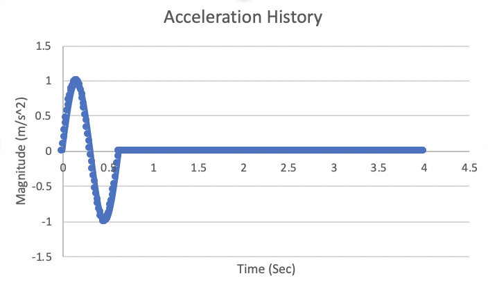
Figure 1: Acceleration history prescribed at the base of the soil column.
At this point, we will start going through the input file. Each block of text in the input file will be briefly explained and useful links will be provided for further investigation.
[GlobalParams<<<{"href": "../syntax/GlobalParams/index.html"}>>>]
  displacements = 'disp_x disp_y disp_z'
[]The first block shown in this input file is the Global Params. This is an optional block of text in the MASTODON input file, which is useful for defining parameters that are required in multiple blocks of the input file. Instead of defining these parameters in each of the blocks that require it, you can define it only once in the GlobalParams block. In general this will help the user shorten his or her input file, but is not at all a requirement. In this instance, we have defined the displacement variables, which are required to be defined in the dynamic tensor mechanics kernel and the strain calculator block. Instead of defining them in those two places, we can define them only once in GlobalParams. The redundant lines are commented in the input file to show where they would be, if not set in the GlobalParams block.
[Mesh<<<{"href": "../syntax/Mesh/index.html"}>>>]
  type = GeneratedMesh
  nx = 1
  ny = 1
  nz = 100
  xmin = -0.5
  ymin = -0.5
  zmin = 0.0
  xmax = 0.5
  ymax = 0.5
  zmax = 100.0
  dim = 3
[]The next block in the input file is the Mesh block. This is a required block of text in the input file where the user defines the mesh to be used in the analysis. For simple geometry, the mesh can be created using the internal mesh generator which is the method demonstrated in this input file. The model is a 100 m soil column containing 100 elements, each measuring 1 m x 1 m x 1 m. If the geometry is more complex than rectangle/cube shapes, it is advised that the user create the mesh using an external mesh generation software. Mesh files can be imported in this block by changing the type to FileMesh. Users and developers at INL utilize Cubit for most of our mesh generation needs, which is commercially available as Trelis. The preferred file type is an exodus (.e) file, although MASTODON can support other mesh file types, such as Abaqus (.inp) files (some limitations apply). See Mesh for more information on the mesh system.
[Variables<<<{"href": "../syntax/Variables/index.html"}>>>]
  [./disp_x]
  [../]
  [./disp_y]
  [../]
  [./disp_z]
  [../]
[]The next block of text is the Variables block. This is where the user defines the non-linear variables being solved for, such as displacements, temperature, etc. See Variables for more information on the variables system.
[AuxVariables<<<{"href": "../syntax/AuxVariables/index.html"}>>>]
  [./vel_x]
  [../]
  [./accel_x]
  [../]
  [./vel_y]
  [../]
  [./accel_y]
  [../]
  [./vel_z]
  [../]
  [./accel_z]
  [../]
  [./layer_id]
  [../]
[]Following Variables, the user must then define the AuxVariables. Auxiliary variables are values which can be derived from the primary variables or explicitly defined, this includes velocity, acceleration, stress etc. See AuxVariables for more information on the AuxVariables system.
[Kernels<<<{"href": "../syntax/Kernels/index.html"}>>>]
  [./DynamicTensorMechanics<<<{"href": "../syntax/Kernels/DynamicTensorMechanics/index.html"}>>>]
    # displacements = 'disp_x disp_y disp_z'
  [../]
  [./inertia_x]
    type = InertialForce<<<{"description": "Calculates the residual for the inertial force ($M \\cdot acceleration$) and the contribution of mass dependent Rayleigh damping and HHT time  integration scheme ($\\eta \\cdot M \\cdot ((1+\\alpha)velq2-\\alpha \\cdot vel-old) $)", "href": "../source/kernels/InertialForce.html"}>>>
    variable<<<{"description": "The name of the variable that this residual object operates on"}>>> = disp_x
    velocity<<<{"description": "velocity variable"}>>> = vel_x
    acceleration<<<{"description": "acceleration variable"}>>> = accel_x
    beta<<<{"description": "beta parameter for Newmark Time integration"}>>> = 0.25
    gamma<<<{"description": "gamma parameter for Newmark Time integration"}>>> = 0.5
  [../]
  [./inertia_y]
    type = InertialForce<<<{"description": "Calculates the residual for the inertial force ($M \\cdot acceleration$) and the contribution of mass dependent Rayleigh damping and HHT time  integration scheme ($\\eta \\cdot M \\cdot ((1+\\alpha)velq2-\\alpha \\cdot vel-old) $)", "href": "../source/kernels/InertialForce.html"}>>>
    variable<<<{"description": "The name of the variable that this residual object operates on"}>>> = disp_y
    velocity<<<{"description": "velocity variable"}>>> = vel_y
    acceleration<<<{"description": "acceleration variable"}>>> = accel_y
    beta<<<{"description": "beta parameter for Newmark Time integration"}>>> = 0.25
    gamma<<<{"description": "gamma parameter for Newmark Time integration"}>>> = 0.5
  [../]
  [./inertia_z]
    type = InertialForce<<<{"description": "Calculates the residual for the inertial force ($M \\cdot acceleration$) and the contribution of mass dependent Rayleigh damping and HHT time  integration scheme ($\\eta \\cdot M \\cdot ((1+\\alpha)velq2-\\alpha \\cdot vel-old) $)", "href": "../source/kernels/InertialForce.html"}>>>
    variable<<<{"description": "The name of the variable that this residual object operates on"}>>> = disp_z
    velocity<<<{"description": "velocity variable"}>>> = vel_z
    acceleration<<<{"description": "acceleration variable"}>>> = accel_z
    beta<<<{"description": "beta parameter for Newmark Time integration"}>>> = 0.25
    gamma<<<{"description": "gamma parameter for Newmark Time integration"}>>> = 0.5
  [../]
[]The Kernels block is where the physics of interest is defined. Because MASTODON is built on the MOOSE Framework, it can accomodate many types of problems, and therefore does not expect dynamics problems only. Because this is a dynamics simulation, the user must define the DynamicTensorMechanics block, along with the inertia blocks for the three directions. There is a large library of options for this block in the input file. See Kernels for more information on the Kernels system.
[AuxKernels<<<{"href": "../syntax/AuxKernels/index.html"}>>>]
  [./accel_x]
    type = NewmarkAccelAux<<<{"description": "Computes the current acceleration using the Newmark method.", "href": "../source/auxkernels/NewmarkAccelAux.html"}>>>
    variable<<<{"description": "The name of the variable that this object applies to"}>>> = accel_x
    displacement<<<{"description": "displacement variable"}>>> = disp_x
    velocity<<<{"description": "velocity variable"}>>> = vel_x
    beta<<<{"description": "beta parameter for Newmark method"}>>> = 0.25
    execute_on<<<{"description": "The list of flag(s) indicating when this object should be executed. For a description of each flag, see https://mooseframework.inl.gov/source/interfaces/SetupInterface.html."}>>> = timestep_end
  [../]
  [./vel_x]
    type = NewmarkVelAux<<<{"description": "Calculates the current velocity using Newmark method.", "href": "../source/auxkernels/NewmarkVelAux.html"}>>>
    variable<<<{"description": "The name of the variable that this object applies to"}>>> = vel_x
    acceleration<<<{"description": "acceleration variable"}>>> = accel_x
    gamma<<<{"description": "gamma parameter for Newmark method"}>>> = 0.5
    execute_on<<<{"description": "The list of flag(s) indicating when this object should be executed. For a description of each flag, see https://mooseframework.inl.gov/source/interfaces/SetupInterface.html."}>>> = timestep_end
  [../]
  [./accel_y]
    type = NewmarkAccelAux<<<{"description": "Computes the current acceleration using the Newmark method.", "href": "../source/auxkernels/NewmarkAccelAux.html"}>>>
    variable<<<{"description": "The name of the variable that this object applies to"}>>> = accel_y
    displacement<<<{"description": "displacement variable"}>>> = disp_y
    velocity<<<{"description": "velocity variable"}>>> = vel_y
    beta<<<{"description": "beta parameter for Newmark method"}>>> = 0.25
    execute_on<<<{"description": "The list of flag(s) indicating when this object should be executed. For a description of each flag, see https://mooseframework.inl.gov/source/interfaces/SetupInterface.html."}>>> = timestep_end
  [../]
  [./vel_y]
    type = NewmarkVelAux<<<{"description": "Calculates the current velocity using Newmark method.", "href": "../source/auxkernels/NewmarkVelAux.html"}>>>
    variable<<<{"description": "The name of the variable that this object applies to"}>>> = vel_y
    acceleration<<<{"description": "acceleration variable"}>>> = accel_y
    gamma<<<{"description": "gamma parameter for Newmark method"}>>> = 0.5
    execute_on<<<{"description": "The list of flag(s) indicating when this object should be executed. For a description of each flag, see https://mooseframework.inl.gov/source/interfaces/SetupInterface.html."}>>> = timestep_end
  [../]
  [./accel_z]
    type = NewmarkAccelAux<<<{"description": "Computes the current acceleration using the Newmark method.", "href": "../source/auxkernels/NewmarkAccelAux.html"}>>>
    variable<<<{"description": "The name of the variable that this object applies to"}>>> = accel_z
    displacement<<<{"description": "displacement variable"}>>> = disp_z
    velocity<<<{"description": "velocity variable"}>>> = vel_z
    beta<<<{"description": "beta parameter for Newmark method"}>>> = 0.25
    execute_on<<<{"description": "The list of flag(s) indicating when this object should be executed. For a description of each flag, see https://mooseframework.inl.gov/source/interfaces/SetupInterface.html."}>>> = timestep_end
  [../]
  [./vel_z]
    type = NewmarkVelAux<<<{"description": "Calculates the current velocity using Newmark method.", "href": "../source/auxkernels/NewmarkVelAux.html"}>>>
    variable<<<{"description": "The name of the variable that this object applies to"}>>> = vel_z
    acceleration<<<{"description": "acceleration variable"}>>> = accel_z
    gamma<<<{"description": "gamma parameter for Newmark method"}>>> = 0.5
    execute_on<<<{"description": "The list of flag(s) indicating when this object should be executed. For a description of each flag, see https://mooseframework.inl.gov/source/interfaces/SetupInterface.html."}>>> = timestep_end
  [../]
  [./layer_id]
     type = UniformLayerAuxKernel<<<{"description": "Computes an AuxVariable for representing a layered structure in an arbitrary direction.", "href": "../source/auxkernels/UniformLayerAuxKernel.html"}>>>
     variable<<<{"description": "The name of the variable that this object applies to"}>>> = layer_id
     interfaces<<<{"description": "A list of layer interface locations to apply across the domain in the specified direction."}>>> = '20 60 100.1'
     direction<<<{"description": "The direction to apply layering."}>>> = '0.0 0.0 1.0'
     execute_on<<<{"description": "The list of flag(s) indicating when this object should be executed. For a description of each flag, see https://mooseframework.inl.gov/source/interfaces/SetupInterface.html."}>>> = initial
  [../]
[]The AuxKernels block is defined next. AuxKernels act on variables using explicit or know functions in order to determine the AuxVariable values. Here is where we define all accelerations and velocities, which are determined using the displacement variables in the Newmark Method. This block is also where stress or other field variables would be setup. See AuxKernels for more information on the AuxKernels system.
[BCs<<<{"href": "../syntax/BCs/index.html"}>>>]
  [./bottom_z]
    type = DirichletBC<<<{"description": "Imposes the essential boundary condition $u=g$, where $g$ is a constant, controllable value.", "href": "../source/bcs/DirichletBC.html"}>>>
    variable<<<{"description": "The name of the variable that this residual object operates on"}>>> = disp_z
    boundary<<<{"description": "The list of boundary IDs from the mesh where this object applies"}>>> = 'back'
    value<<<{"description": "Value of the BC"}>>> = 0.0
  [../]
  [./bottom_y]
    type = DirichletBC<<<{"description": "Imposes the essential boundary condition $u=g$, where $g$ is a constant, controllable value.", "href": "../source/bcs/DirichletBC.html"}>>>
    variable<<<{"description": "The name of the variable that this residual object operates on"}>>> = disp_y
    boundary<<<{"description": "The list of boundary IDs from the mesh where this object applies"}>>> = 'back'
    value<<<{"description": "Value of the BC"}>>> = 0.0
  [../]
  [./bottom_accel]
    type = PresetAcceleration<<<{"description": "Prescribe acceleration on a given boundary in a given direction", "href": "../source/bcs/PresetAcceleration.html"}>>>
    boundary<<<{"description": "The list of boundary IDs from the mesh where this object applies"}>>> = 'back'
    function<<<{"description": "Function describing the velocity."}>>> = accel_bottom
    variable<<<{"description": "The name of the variable that this residual object operates on"}>>> = 'disp_x'
    beta<<<{"description": "beta parameter for Newmark time integration."}>>> = 0.25
    acceleration<<<{"description": "The acceleration variable."}>>> = 'accel_x'
    velocity<<<{"description": "The velocity variable."}>>> = 'vel_x'
  [../]
  [./Periodic<<<{"href": "../syntax/BCs/Periodic/index.html"}>>>]
    [./y_dir]
      variable<<<{"description": "Variable for the periodic boundary condition"}>>> = 'disp_x disp_y disp_z'
      primary<<<{"description": "Boundary ID associated with the primary boundary."}>>> = 'bottom'
      secondary<<<{"description": "Boundary ID associated with the secondary boundary."}>>> = 'top'
      translation<<<{"description": "Vector that translates coordinates on the primary boundary to coordinates on the secondary boundary."}>>> = '0.0 1.0 0.0'
    [../]
    [./x_dir]
      variable<<<{"description": "Variable for the periodic boundary condition"}>>> = 'disp_x disp_y disp_z'
      primary<<<{"description": "Boundary ID associated with the primary boundary."}>>> = 'left'
      secondary<<<{"description": "Boundary ID associated with the secondary boundary."}>>> = 'right'
      translation<<<{"description": "Vector that translates coordinates on the primary boundary to coordinates on the secondary boundary."}>>> = '1.0 0.0 0.0'
    [../]
  [../]
[]Now that all of the variables have been defined and set up properly, we can begin to formulate the problem for the analysis. The BCs block is where problem boundary conditions are applied. We use the DirichletBC type to fix the bottom surface of the soil column in the Y and Z directions, then prescribe an acceleration history to the bottom surface using the PresetAcceleration type. This is defined in the X direction only, for this problem. In order to constrain the soil column so that it only moves in shear, a periodic boundary condition is applied along the side surfaces of the soil column using the Periodic block. The side surfaces are input as boundaries. The boundaries called 'back', 'front', 'bottom', and 'top' are automatically created by the GeneratedMesh above. Usually, these boundaries will have to be defined in Cubit, Trelis, or any other meshing software being used. The Periodic BC requires the surfaces (input as boundaries) to be perfectly parallel and the normal vector of translation between the surfaces is input as the 'translation' parameter. See BCs for more information on the boundary conditions system including the Periodic BC.
[Functions<<<{"href": "../syntax/Functions/index.html"}>>>]
  [./accel_bottom]
     type = PiecewiseLinear<<<{"description": "Linearly interpolates between pairs of x-y data", "href": "../source/functions/PiecewiseLinear.html"}>>>
     data_file<<<{"description": "File holding CSV data"}>>> = 'acceleration_hist.csv'
     format<<<{"description": "Format of csv data file that is in either in columns or rows"}>>> = 'columns'
  [../]
[]The next block in this input file is the Functions block. This is another optional block that is not required for all simulations. Recall from the boundary conditions that for this model we are prescribing the base acceleration. There are a number of ways to do this within MASTODON, one of which is to supply a csv file that contains the acceleration history to be used. We input this file using a PiecewiseLinear function so that if the timesteps in the simulation do not exactly match those of the acceleration history, the acceleration values will be linearly interpolated. There are a wide variety of function types that can be defined within this block. See Functions for more information.
[Materials<<<{"href": "../syntax/Materials/index.html"}>>>]
  [./linear_soil]
    type = ComputeIsotropicElasticityTensorSoil<<<{"description": "Compute an isotropic elasticity tensor for a layered soil material when shear modulus or elastic modulus, poisson's ratio and density are provided as input for each layer.", "href": "../source/materials/ComputeIsotropicElasticityTensorSoil.html"}>>>
    layer_variable<<<{"description": "The variable providing the soil layer identification."}>>> = layer_id
    layer_ids<<<{"description": "Vector of layer ids that map one-to-one with the 'shear_modulus' or 'elastic_modulus', 'poissons_ratio' and 'density' input parameters."}>>> = '0 1 2'
    shear_modulus<<<{"description": "Vector of shear modulus values that map one-to-one with the number 'layer_ids' parameter."}>>> = '3e6 2e6 1e6'
    poissons_ratio<<<{"description": "Vector of Poisson's ratio values that map one-to-one with the number 'layer_ids' parameter."}>>> = '0.2 0.2 0.2'
    density<<<{"description": "Vector of density values that map one-to-one with the number 'layer_ids' parameter."}>>> = '1200 1000 800'
  [../]
  [./strain]
    type = ComputeSmallStrain<<<{"description": "Compute a small strain.", "href": "../source/materials/ComputeSmallStrain.html"}>>>
    # displacements = 'disp_x disp_y disp_z'
  [../]
  [./stress]
    type = ComputeLinearElasticStress<<<{"description": "Compute stress using elasticity for small strains", "href": "../source/materials/ComputeLinearElasticStress.html"}>>>
  [../]
[]The materials block is a required block in the MASTODON input file. This is where the user will define the material models to be used and the property values necessary for those calculations. For this example we have one block of material, which is linear soil. We define the material type as ComputeIsotropicElasticityTensorSoil and define the necessary properties for each soil layer. Additionally we define the stress and strain formulations. There are a great deal of material options available to MASTODON users, see Materials for more information on the materials system.
[Executioner<<<{"href": "../syntax/Executioner/index.html"}>>>]
  type = Transient
  solve_type = NEWTON
  start_time = 0
  end_time = 4
  dt = 0.01
  timestep_tolerance = 1e-6
[]The Executioner is a required block in the input file. It defines important solver information, start and end times, convergence criteria and timestep size. See Executioner for more information on the executioner system.
[Postprocessors<<<{"href": "../syntax/Postprocessors/index.html"}>>>]
  [top_ax_pv]
    type = PointValue<<<{"description": "Compute the value of a variable at a specified location", "href": "../source/postprocessors/PointValue.html"}>>>
    point<<<{"description": "The physical point where the solution will be evaluated."}>>> = '0 0 100'
    variable<<<{"description": "The name of the variable that this postprocessor operates on."}>>> = 'accel_x'
  []
  [./top_ax_nvv]
    type = NodalVariableValue<<<{"description": "Outputs values of a nodal variable at a particular location", "href": "../source/postprocessors/NodalVariableValue.html"}>>>
    variable<<<{"description": "The variable to be monitored"}>>> = accel_x
    nodeid<<<{"description": "The ID of the node where we monitor"}>>> = 401
  [../]
[]The Postprocessors block is another optional block in the input file. It is useful for obtaining various quantities of interest. For instance, if the user would like to get the acceleration history at the top of the soil column, there are a number of ways to do that. One way would be to run the analysis without any postprocessors, then probe the field values in an exodus viewer such as paraview. Another method, is to use a postprocessor in MASTODON. In this input file, we have two postprocessors defined, but both do the same thing - obtain the acceleration history at the top of the soil column. The data collected is output in a csv file. There are several postprocessors available for use in MASTODON, for more information see Postprocessors.
[VectorPostprocessors<<<{"href": "../syntax/VectorPostprocessors/index.html"}>>>]
  [./accel_hist]
    type = ResponseHistoryBuilder<<<{"description": "Calculates response histories for a given node and variable(s).", "href": "../source/vectorpostprocessors/ResponseHistoryBuilder.html"}>>>
    variables<<<{"description": "Variable name for which the response history is requested."}>>> = 'accel_x accel_y accel_z'
    nodes<<<{"description": "Node number(s) at which the response history is needed."}>>> = '401'
  [../]
  [./accel_spec]
    type = ResponseSpectraCalculator<<<{"description": "Calculate the response spectrum at the requested nodes or points.", "href": "../source/vectorpostprocessors/ResponseSpectraCalculator.html"}>>>
    vectorpostprocessor<<<{"description": "Name of the ResponseHistoryBuilder vectorpostprocessor, for which response spectra are calculated."}>>> = accel_hist
    regularize_dt<<<{"description": "dt for response spectra calculation. The acceleration response will be regularized to this dt prior to the response spectrum calculation."}>>> = 0.01
    # outputs = out
  [../]
[]Similar to Postprocessors, the user can also define vectorpostprocessors. These can be thought of as postprocessors that define multiple values at each step in the simulation. In this input we have setup the ResponseHistoryBuilder in order to obtain the acceleation histories at the top of the soil column, and the ResponseSpectraCalculator in order to obtain the response spectra for each of those acceleration histories. Like postprocessors, there are a wide variety of VectorPostprocessors available for use in MASTODON. See VectorPostprocessors for more information.
[Outputs<<<{"href": "../syntax/Mastodon/Outputs/index.html"}>>>]
  csv<<<{"description": "Output the scalar variable and postprocessors to a *.csv file using the default CSV output."}>>> = true
  exodus<<<{"description": "Output the results using the default settings for Exodus output."}>>> = true
[]The final block of text in this input file is the Outputs block. It is not required, and some information is automatically output by default. This block is useful for controlling the amount of information that is output to the screen during your simulation, as well as other useful information such as performance metrics. This is also where the user can specify the types of files to be output (csv, exodus, etc.). See Outputs for more information on the outputs system.
In general, an exodus file is the output file that will be useful for visualization of the results. For this, any exodus file viewing software will work. Peacock is the MOOSE Graphical User Interface currently being developed and used within the MOOSE developer and user community. Another option that is widely used is Paraview.