ver-1dc
Permeation Problem with Multiple Trapping
Test Description
This verification problem is taken from Ambrosek and Longhurst (2008) and builds on the capabilities verified in ver-1d. However, in the current case, there are three different types of traps. This case is simulated in (test/tests/ver-1dc/ver-1dc.i).
This problem models permeation through a membrane with a constant source in which three trap populations are present. We solve the following equations
(1) and, for , , and : (2) and (3) where is the concentrations of the mobile, is the trapped species in trap , is the diffusivity of the mobile species, and are the trapping and release rate coefficients for trap , is a factor scaling to be closer to for better numerical convergence, is the fraction of host sites that can contribute to trapping, is the concentration of empty trapping sites, and is the host density.
The trapping parameter is defined by (4)
where
= lattice parameter
= Debye frequency ( )
= trapping site fraction
= diffusivity pre-exponential
= diffusion activation energy
= trap energy
= Boltzmann's constant
= temperature
and = dissolved gas atom fraction.
This verification case was first introduced in Ambrosek and Longhurst (2008) to highlight TMAP7's capability to model up to three different trapping populations, when TMAP4 was limited to one (Longhurst et al., 1992). However, TMAP8 can accommodate an arbitrary number of trapping populations.
Three traps that are relatively weak are assumed to be active in a slab. The trapping site fraction of the three traps are 0.1, 0.15 and 0.20, respectively. The values of for the three traps are 100 K, 500 K, and 800 K, respectively. Other parameters are the same as the trap in the effective diffusivity limit in ver-1d.
Analytical solution
Ambrosek and Longhurst (2008) provides the analytical equations for the permeation transient as
(5) where is the steady dissolved gas concentration at the upstream (x = 0) side, is the thickness of the slab, is the diffusivity of the gas through the material, and , the breakthrough time, is defined as
(6) where , the effective diffusivity, is defined as
(7) where is the trapping parameter of trap . The trapping parameters, , calculated from Eq. (4) for the three traps are 91.47930 , 61.65009 , 45.93069 .
The values of the three traps from Ambrosek and Longhurst (2008) have a typographical error: They are three orders of magnitude lower than the correct values. However, it does not impact the final analytical solution.
Results and comparison against analytical solution
The analytical solution for the permeation transient is compared with TMAP8 results in Figure 1. The graphs for the theoretical flux and the calculated flux are in good agreement, with root mean square percentage errors (RMSPE) of RMSPE = 0.41 % for s. The breakthrough time calculated from Eq. (6) in analytical solution is 4.04 s, and the breakthrough time from TMAP8 is 4.12 s.
.](figures/ver-1dc_comparison_diffusion.png)
Figure 1: Comparison of TMAP8 calculation with the analytical solution for the permeation transient from Ambrosek and Longhurst (2008).
Further verification using the method of manufactured solutions (MMS)
Although the flux and breakthrough time can be verified using analytical solutions as presented above, the MMS approach is a powerful method to verify complex systems of PDEs such as the one studied in this case. Here, we apply the MMS approach available as a Python-based utility in the MOOSE framework to verify TMAP8's predictions for ver-1dc through spatial convergence.
The derivation of the weak forms of the system of equations in Eq. (1) and Eq. (2) is detailed in TMAP8's theory manual. With the weak forms of the equations, we can apply the MMS. Below, we (1) detail how we apply the MMS approach to this case, and (2) discuss the results.
Application of the MMS
A detailed and step by step description of the MMS approach is available on the MOOSE MMS page. To perform a spatial convergence study with the MMS, we select a smoothly-varying sinusoidal spatial solution for the mobile and trapped species. In order to prevent temporal error from polluting the spatial error, we pick a temporal dependence that can be exactly represented by the time integrator we choose. In this MMS case, we use implicit or backwards Euler which is first-order accurate; consequently we choose a linear dependence on time. For our 1D case, this leads us to select the following MMS solution for the mobile species:
(8)
with the position along the 1D domain, and the time. The trapping species concentrations are represented similarly with, for , , and :
(9)
with the equivalent of in Eq. (3).
With the manufactured solutions selected, we generate forcing functions and by substituting the exact solutions into the strong-form PDEs, Eq. (1) and Eq. (2), leading to (assuming ):
(10) and, for , , and : (11)
and are therefore defined as:
(12) and, for , , and : (13)
Eq. (10) and Eq. (11) now form a system of equations that can be solved and compared against the exact solutions defined in Eq. (8) and Eq. (9).
These forcing functions are then imposed in the TMAP8 input file using BodyForce and UserForcingFunctionNodalKernel, respectively. Dirichlet boundary conditions for the mobile species are imposed using the selected exact/MMS solution. For the spatial discretization, we select first order Lagrange basis functions for the mobile concentration and for projecting the trapped species concentrations from nodes into element interiors for coupling in the trapped specie time derivative term in the mobile specie governing equation.
Results
The results of the spatial convergence study using the MMS is shown in Figure 2, with 10 levels of refinement. The expected quadratic convergence rate of the error is observed, hence verifying the proper implementation of the diffusion and multi-trapping capabilities.
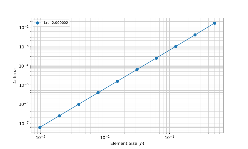
Figure 2: Spatial convergence for a diffusion-trapping-release problem modeled after the physics of ver-1dc using first order Lagrange basis functions. The expected quadratic convergence rate of the error is observed.
Input files
This case contains several input files. For the verification using the comparison against the analytical solutions, the input file can be found at (test/tests/ver-1dc/ver-1dc.i). For the verification using the MMS, the input file can be found at (test/tests/ver-1dc/ver-1dc_mms.i). The (test/tests/ver-1dc/test.py) script runs the MMS test using (test/tests/ver-1dc/ver-1dc_mms.i). Note that both input files utilize the base input file (test/tests/ver-1dc/ver-1dc_base.i), which contains all the objects that both verification approach share. Using a base input file such as (test/tests/ver-1dc/ver-1dc_base.i) reduces redundancy, eases maintenance, and ensures consistency between the two verification set ups.
Note that to limit the computational costs of the test cases, the tests run a version of (test/tests/ver-1dc/ver-1dc.i) with a coarser mesh and fewer time steps. More information about the changes can be found in the test specification file for this case (test/tests/ver-1dc/tests).
References
- James Ambrosek and GR Longhurst.
Verification and Validation of TMAP7.
Technical Report INEEL/EXT-04-01657, Idaho National Engineering and Environmental Laboratory, December 2008.[BibTeX]
- GR Longhurst, SL Harms, ES Marwil, and BG Miller.
Verification and Validation of TMAP4.
Technical Report EGG-FSP-10347, Idaho National Engineering Laboratory, Idaho Falls, ID (United States), 1992.[BibTeX]