Tutorial
Tritium Migration Analysis Program,
Version 8 (TMAP8)
November 2025
Outline of the workshop slides
Goals and Objectives
Introduction to MOOSE
- Overview and key features
- Understanding input files
- Development process and SQA
- Getting help
- Why MOOSE for TMAP8?
Introduction to TMAP8
- TMAP8 Overview and key features
- Theory
- TMAP8 Capabilities
- TMAP8 Verification & Validation
- TMAP8 Examples
TMAP8 Verification Walkthrough
- Go through diffusion and trapping verification case
Getting started with TMAP8
- Installing TMAP8
- Run a verification case
- Visualize results
Concluding Remarks (Q&A, Feedback, Future discussions)
Workshop Goals & Objectives
Goals
Provide introductory information about MOOSE and TMAP8.
Empower participants to confidently begin exploring and using TMAP8 and MOOSE.
Provide a hands-on learning experience with real examples.
Lead participants through working with and changing input files.
Help participants navigate resources and communities for continued learning.
Objectives
By the end of this workshop slides, participants will:
Understand the purpose and capabilities of MOOSE and TMAP8.
Successfully install TMAP8.
Run and modify simulations, as well as plot and analyze results.
Identify and access documentation, tutorials, and community support.
Leave with a clear path for continued use and development.
Introduction to MOOSE
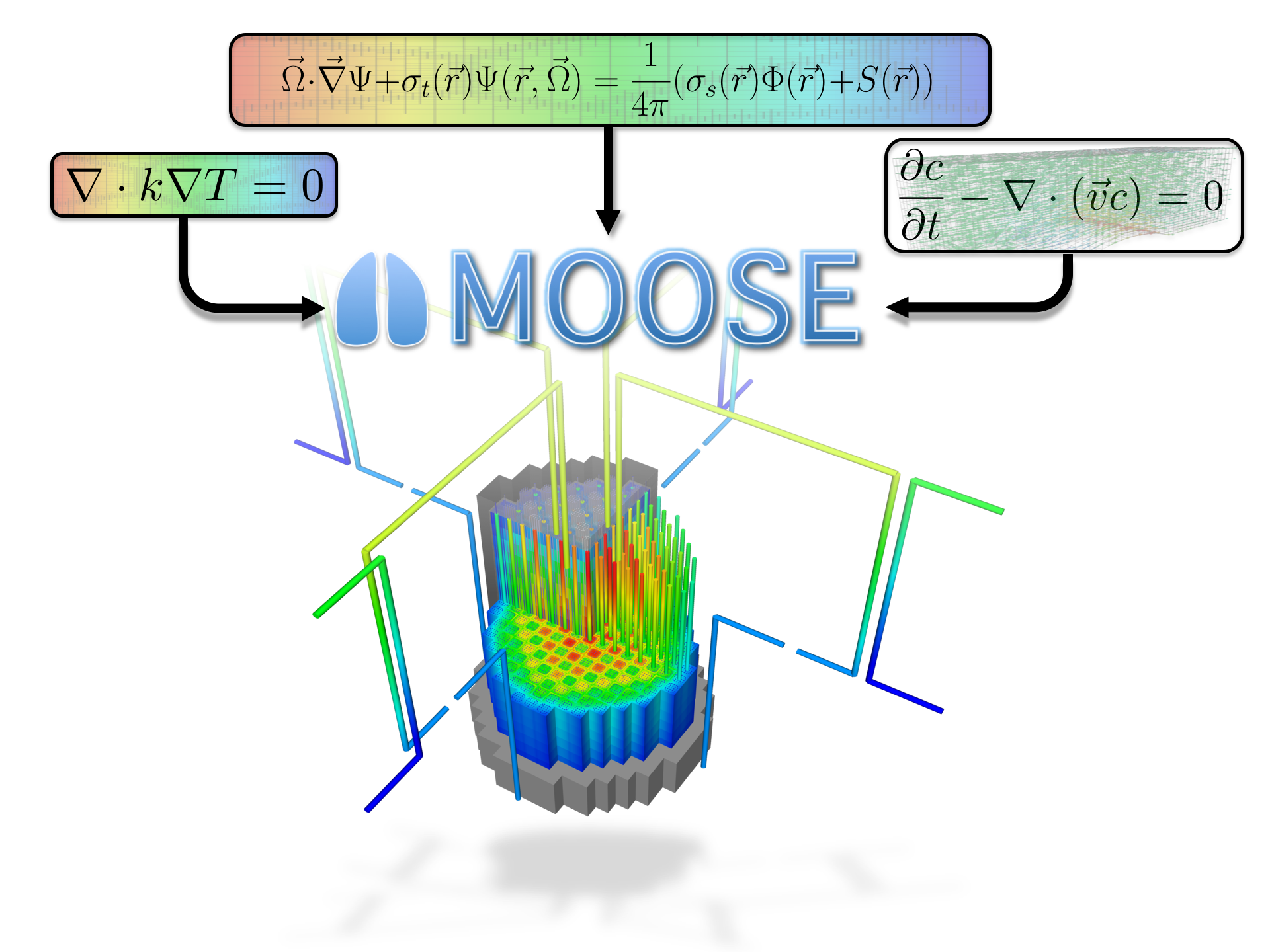
MOOSE Framework: Overview
Developed by Idaho National Laboratory since 2008
Used for studying and analyzing nuclear reactor problems
Free and open source (LGPLv2 license)
Large user community (5000+ unique visitors/month)
Highly parallel and HPC capable
Developed and supported by full time INL staff - long-term support
https://www.mooseframework.inl.gov
MOOSE Framework: Key features
Massively parallel computation - successfully run on >100,000 processor cores
Multiphysics solve capability - fully coupled and implicit solver
Multiscale solve capability - multiple applications can perform computation for a problem simultaneously
Provides high level interface to implement customized physics, geometries, boundary conditions, and material models
Initially developed to support nuclear R&D but now widely used for non-nuclear R&D also
MOOSE Framework: Core Philosophy
Object-oriented design : Everything is an object with clear interfaces
Modular architecture : Mix and match components and/or physics to achieve simulation goals
Supporting Many Physics : Framework handles numerics, you focus on physics
Dimension-independent : Run in 1D, 2D, or 3D with minimal changes to the input file
Automatic differentiation : No need to compute Jacobians manually
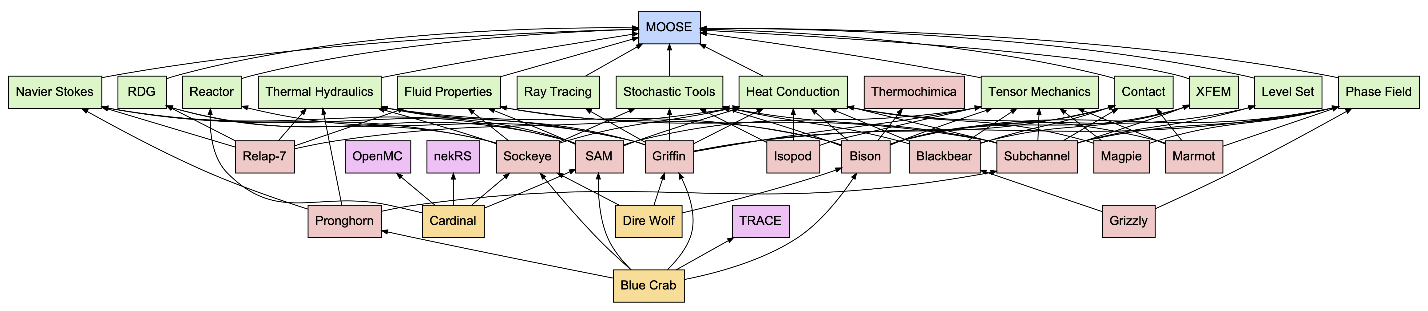
MOOSE Framework: Applications
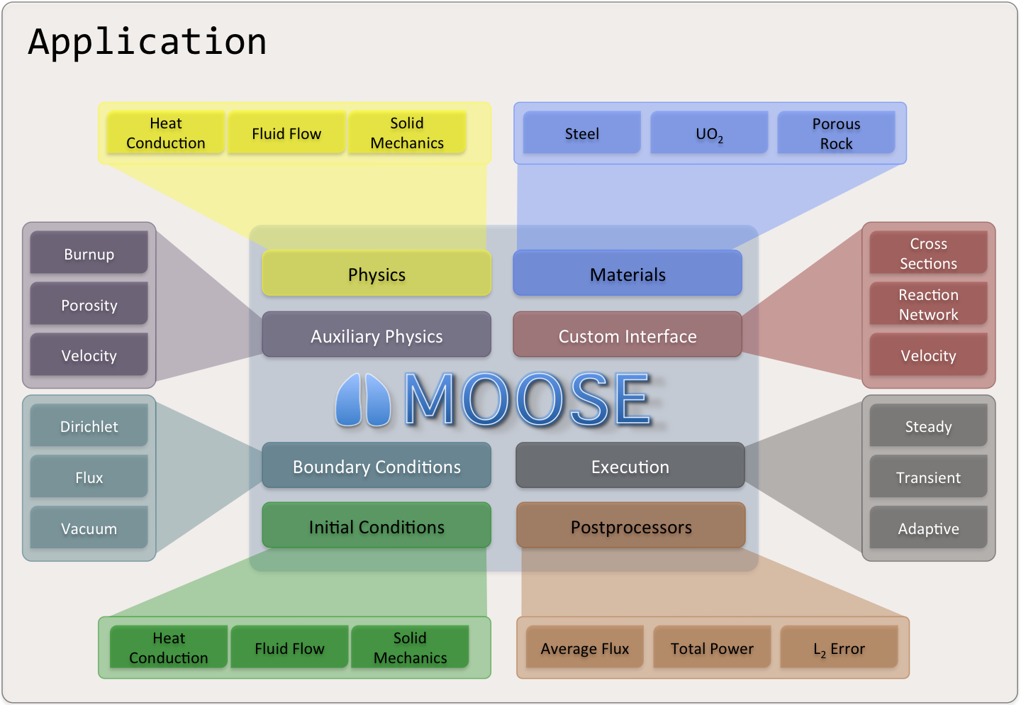
MOOSE Systems Architecture
Core Systems:
Mesh
Variables
Kernels
BCs
Materials
AuxKernels
Functions
Advanced Systems:
MultiApps (multi-scale coupling)
Transfers (data exchange)
Postprocessors (scalar values)
VectorPostprocessors (vector values)
UserObjects (custom algorithms)
Controls (runtime parameter modification)
Executioner (solve control)
Each system has specific responsibilities
Systems interact through well-defined interfaces
Objects can be mixed and matched
MOOSE Systems Architecture
example for a TMAP8-relevant case
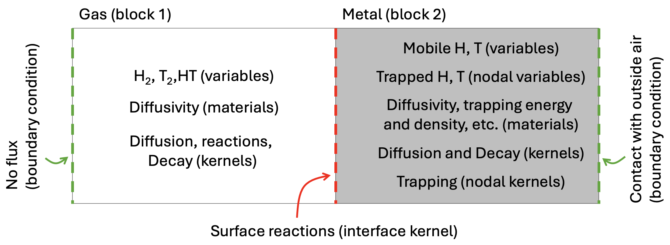
The upcoming slides will describe the main components of the MOOSE systems architecture. This slide illustrates in which context different systems are used in a TMAP8-relevant case.
Let's assume one wants to model hydrogen and tritium transport through the metallic walls of a pipe. The model would include diffusion, decay, and reactions between diatomic molecules inside the pipe; surface reactions at the inner and outer walls; and diffusion, decay, and trapping for single atoms in the walls. The figure below illustrates the case and specifies how MOOSE's systems would apply when constructing the case in a MOOSE input file:
The Finite Element Method in MOOSE
MOOSE solves PDEs using the Galerkin finite element method (the finite volume method is also available for fluid flow).
Key steps:
Write strong form of PDE
Convert to weak form (multiply by test function, integrate by parts)
Discretize with shape functions
Form residual vector and Jacobian matrix
Solve nonlinear system with Newton's method
MOOSE handles:
Mesh management
Shape functions
Quadrature rules
Assembly process
Parallel decomposition
Example: Strong form, weak form, and implementation

Kernels System: Building PDEs
class DiffusionKernel : public ADKernel
{
protected:
  virtual ADReal computeQpResidual() override
  {
    return _grad_test[_i][_qp] * _grad_u[_qp];
  }
};
Kernels represent volume terms in PDEs
Each kernel computes one term
Automatic differentiation for Jacobians
Mix kernels to build complex equations
Available variables:
_u,_grad_u: Variable value and gradient_test,_grad_test: Test function value and gradient_qp: Quadrature point index_q_point: Physical coordinates
Special Note: NodalKernels System
Purpose: Compute residual contributions at nodes rather than quadrature points
When to Use NodalKernels:
Non-diffusive species
ODEs or time-derivative only terms
Point sources or sinks
Reaction terms without spatial derivatives
Lumped parameter models
Key Differences from Kernels:
Operates on nodes, not elements
No spatial gradients available
_qp = 0always (single evaluation point)No test function needed in residual
More efficient for non-spatial terms
Implementation:
  ADReal
  ReactionNodalKernel::computeQpResidual()
  {
    // Note: _qp = 0 for nodal kernels
    // (evaluated at only a single point)
    return _coef * _u[_qp];
  }
};
Input File Example:
[NodalKernels]
  ...
  [decay]
    type = ReactionNodalKernel
    variable = C_tritium
    coef = 1.0
  []
[]
NodalKernels in TMAP8
Nodal kernels are used to model non-diffusive species. In the case of TMAP8, nodal kernels are key to modeling trapped species. For example, these are used in the Ver-1d verification case and several validation cases.
Application Examples:
Trap filling/release (Ver-1d)
Surface reactions at nodes
Materials System: Property Management
Producer/Consumer Pattern:
Materials produce properties than can be used in the rest of the simulation
Other objects (including other materials), can consume properties
Properties can vary in space and time
Properties can be functions of variables or other properties
// Material object, in the constructor
_permeability(declareADProperty<Real>("permeability"))
// In the compute method
_permeability = 2.0;

// Consumer object (Kernel, BCs, etc.) in the constructor
_permeability(getADMaterialProperty<Real>("permeability"))

// In the "computeQp..." method
ADReal
SomeObject::computeQpResidual() {
return _permability[_qp] * _grad_u[_qp] * _grad_test[_qp];
}
Key Methods:
declareProperty<Type>()- produce a standard material property in a material objectgetMaterialProperty<Type>()- consume a standard material property in a MOOSE objectdeclareADProperty<Type>()- produce an AD material property in a material objectgetADMaterialProperty<Type>()- consume an AD material property in a MOOSE object
Boundary Condition System
Purpose: Apply constraints at domain boundaries
Mathematical Forms:
Dirichlet: on
Neumann: on
Robin (Mixed): on
Base Classes:
NodalBC: Applied at nodes (Dirichlet)IntegratedBC: Applied over sides (Neumann/Robin)AD versions for automatic differentiation
Common BCs in MOOSE/TMAP8:
DirichletBC: Fixed valueNeumannBC: Fixed fluxFunctionDirichletBC: Time/space varyingVacuumBC: Vacuum boundary condition for diffusive speciesConvectiveFluxBC: Convective heat transferBinaryRecombinationBC: Recombination of atoms into moleculesEquilibriumBC: Sorption laws (Sievert's or Henry's)
TMAP8 BC Example
Binary Recombination
This capability is located in the MOOSE Scalar Transport Module (Link). More information about the surface models available in TMAP8 is available in the theory manual.
Strong form:
Input file:
[BCs]
  [ht_t_left]
    type = BinaryRecombinationBC
    variable = t
    v = h
    Kr = Krht
    boundary = left
  []
[]
TMAP8 BC Example
Binary Recombination (continued)
Source:
#include "BinaryRecombinationBC.h"

registerMooseObject("ScalarTransportApp", BinaryRecombinationBC);

InputParameters
BinaryRecombinationBC::validParams()
{
  auto params = ADIntegratedBC::validParams();
  params.addClassDescription("Models recombination of the variable with a coupled species at "
                             "boundaries, resulting in loss");
  params.addRequiredCoupledVar("v", "The other mobile variable that takes part in recombination");
  params.addParam<MaterialPropertyName>(
      "Kr", "Kr", "The name of the material property for the recombination coefficient");
  return params;
}

BinaryRecombinationBC::BinaryRecombinationBC(const InputParameters & parameters)
  : ADIntegratedBC(parameters), _v(adCoupledValue("v")), _Kr(getADMaterialProperty<Real>("Kr"))
{
}

ADReal
BinaryRecombinationBC::computeQpResidual()
{
  return _test[_i][_qp] * _Kr[_qp] * _u[_qp] * _v[_qp];
}
InterfaceKernel System
Purpose: Couple physics across internal interfaces between subdomains
Key Concepts:
Operates on internal subdomain boundaries
Accesses both sides (primary/neighbor)
Used to enforce flux continuity and jump conditions
Applications:
Material interfaces (metal/ceramic)
Phase boundaries
Membrane transport
Contact mechanics
TMAP8 Usage:
Metal/coating permeation barriers
Multi-layer diffusion
Interface trapping/sorption (see theory manual)
TMAP8 Example: InterfaceSorption
Computes a sorption law at the interface between solid and gas in isothermal conditions.
where:
= ideal gas constant (J/mol/K)
= temperature (K)
= solubility (units depend on and )
= pre-exponential constant
= activation energy (J/mol)
= sorption law exponent (1 = Henry's, 1/2 = Sievert's)
InterfaceKernels block in Input File (ver-1kb):
[InterfaceKernels]
  [interface_sorption]
    type = InterfaceSorption
    K0 = ${solubility}
    Ea = 0
    n_sorption = ${n_sorption}
    diffusivity = ${diffusivity}
    unit_scale = ${unit_scale}
    unit_scale_neighbor = ${unit_scale_neighbor}
    temperature = ${temperature}
    variable = concentration_enclosure_1
    neighbor_var = concentration_enclosure_2
    sorption_penalty = 1e1
    boundary = interface
  []
[]
Auxiliary System: Arbitrarily Calculated Variables
Purpose: Variables that are not solved for as part of a PDE/ODE.
Use cases: Postprocessing, visualization, coupling
Auxiliary Variables:
Not solved for directly
Can be computed from other variables
Can be computed directly or imposed
Example: temperature/pressure with a set history
Can be nodal or elemental
Example: Flux Vector from Concentration
Concentration () is a nonlinear variable, computed by the solver.
Diffusive flux () is an auxiliary variable.
Expression is computed via AuxKernel (DiffusionFluxAux)
Another Aux Example: Temperature
This is sampled from the val-2b validation case. First, we need to declare the temperature variable, as we would any other variable. Except, we do it here under the AuxVariables block. Then, we set up an AuxKernel to calculate it using a time-dependent function.
[AuxVariables]
  [temperature]
    initial_condition = ${temperature_initial}
  []
[]
[AuxKernels]
  [temperature_aux]
    type = FunctionAux
    variable = temperature
    function = temperature_bc_func
    execute_on = 'INITIAL LINEAR'
  []
[]
Example, cont.: Aux Temperature in a BC
Now, temperature can be used wherever a regular MooseVariable is used. For example, we use it in val-2b in an EquilibriumBC boundary condition on the left boundary.
[BCs]
  [left_flux]
    type = EquilibriumBC
    Ko = ${solubility_constant_BeO}
    activation_energy = '${fparse solubility_energy_BeO * R}'
    boundary = left
    enclosure_var = enclosure_pressure
    temperature = temperature
    variable = deuterium_concentration_BeO
    p = ${solubility_order}
  []
[]
Input File System: HIT Format
Example: simple_diffusion.i:
[Mesh]
  type = GeneratedMesh
  dim = 2
  nx = 10
  ny = 10
[]

[Variables]
  [u]
  []
[]

[Kernels]
  [diff]
    type = Diffusion
    variable = u
  []
[]

[BCs]
  [left]
    type = DirichletBC
    variable = u
    boundary = left
    value = 0
  []
  [right]
    type = DirichletBC
    variable = u
    boundary = right
    value = 1
  []
[]

[Executioner]
  type = Steady
  solve_type = 'PJFNK'
  petsc_options_iname = '-pc_type -pc_hypre_type'
  petsc_options_value = 'hypre boomeramg'
[]

[Outputs]
  exodus = true
[]
Hierarchical Input Text (HIT):
Block-based structure
Parameters in
key=valueformatStrong typing
Extensive error checking
Documentation built-in
Required blocks:
Mesh
Variables
Kernels
BCs
Executioner
Outputs
Inline Unit Conversions in Input Files
Built-in parser enables calculations and unit conversions directly in input files using the MOOSE fparse and units systems.
${fparse num1 * num2}  # On-the-fly calculations

${units num1 unit1 -> unit2}  # Unit conversions

param = 5.0 * ${top_level_coef1} + ${top_level_coef2}  # Replacements
Available Functions in fparse:
Basic:
+ - * / ^Trig:
sin cos tanExp/Log:
exp log log10Other:
sqrt abs min maxConstants:
pi(3.14159...)
Advantages:
Self-documenting calculations
Avoid external calculators
Useful when performing parametric studies
Version control friendly
Fparse / Units Conversion Usage Example
At the input file top level:
# Diffusion parameters
flux_high = '${units 1e19 at/m^2/s -> at/mum^2/s}'
flux_low = '${units 0      at/mum^2/s}'
diffusivity_coefficient = '${units 4.1e-7 m^2/s -> mum^2/s}'
E_D = '${units 0.39 eV -> J}'
initial_concentration = '${units 1e-10 at/m^3 -> at/mum^3}'
width_source = '${units 3e-9 m -> mum}'
depth_source = '${units 4.6e-9 m -> mum}'
In an object:
[Postprocessors]
  [scaled_flux_surface_right]
    type = ScalePostprocessor
    scaling_factor = '${units 1 m^2 -> mum^2}'
    value = flux_surface_right
    execute_on = 'initial nonlinear linear timestep_end'
    outputs = none
  []
[]
Solver System: PJFNK Method
Preconditioned Jacobian-Free Newton-Krylov (PJFNK)
Newton's Method:
Solves nonlinear system:
Update:
Quadratic convergence
Jacobian-Free:
Approximate operation via finite differences
No explicit Jacobian formation
Reduces memory requirements
Krylov Solvers:
GMRES (default)
Conjuate Gradient (CG), BiCGStab
Build Krylov subspace
Preconditioning:
Hypre/BoomerAMG
Block Jacobi
ILU/LU
Essential for performance
Note that a standard Newton solve (using the exact Jacobian) with preconditioning is also available!
Automatic Differentiation in MOOSE
Benefits:
No manual Jacobian calculations
Reduces development time
Eliminates Jacobian bugs
Maintains accuracy
// Traditional approach
Real computeQpResidual() {...}
Real computeQpJacobian() {...}
Real computeQpOffDiagJacobian() {...}

// AD approach - Jacobian automatic!
ADReal computeQpResidual() {...}
How it works:
Based on the chain rule of partial derivatives
Operator overloading (derivatives propagated with
+,-,*, etc.)"Forward mode" AD
Uses MetaPhysicL library (from the libMesh team)
Best practice:
Use AD kernels/materials
Let MOOSE handle derivatives
More overhead with this method, but much easier to develop!
MultiApp and Transfer Systems
Solving Multiple Applications Together
MultiApp System:
Run multiple MOOSE apps / physics
Different time scales
Different spatial scales
Master/sub-app hierarchy
Use cases:
Multiscale modeling
Multiphysics coupling (when adjustable levels of coupling are desired)
Reduced-order models
Transfer System:
Exchange data between apps
Spatial interpolation
Temporal interpolation
Conservative transfers
Types:
Field transfers
Postprocessor transfers
VectorPostprocessor transfers
Output System
Flexible and Extensible Output
Supported Formats:
Exodus (recommended)
VTK/VTU
CSV (scalar data)
Console
Checkpoint (restart)
Nemesis (parallel)
Input file control:
[Outputs]
  exodus = true
  csv = true
  [custom_out]
    type = Exodus
    interval = 10
    execute_on = 'timestep_end'
  []
[]
Features:
Control output frequency
Select variables to output
Multiple outputs simultaneously
Output control:
By time
By timestep
On events (initial, final, failed)
MOOSE/TMAP8 Development Process
Nuclear Quality Assurance Level 1 (NQA-1)
Version Control:
Git/GitHub workflow
Pull request reviews
Continuous integration
Extensive testing (30M+ tests/week)
Development Tools:
CIVET (testing system)
VSCode integration with language server support
Input file syntax highlighting
Code Standards:
Consistent style (via clang-format)
Documentation required
Test coverage required
Community:
250+ contributors to MOOSE
Testing Framework
TMAP8 Software Quality Assurance Documentation
Test Types:
Exodiff: Compare Exodus filesCSVDiff: Compare CSV outputRunException: Test error conditionsPetscJacobianTester: Verify JacobiansRunApp: Basic execution test
Benefits:
Prevent regressions
Document expected behavior
Enable refactoring
Build confidence
Test Organization:
test/
  tests/
    kernels/
      my_kernel/
        my_kernel.i
        tests
        gold/
          my_kernel_out.e
Test spec (HIT format):
[Tests]
  [my_test]
    type = Exodiff
    input = test.i
    cli_args = 'Kernels/my_kernel/active=true'
    exodiff = test_out.e
  []
[]
Getting Help
Resources Available (all links):
Documentation (MOOSE):
Documentation (TMAP8):
Summary: Why MOOSE for TMAP8?
Proven framework: Used in 500+ publications, tested extensively, production-ready
Parallel scalability: Handles problems from workstation to supercomputer
Multiphysics capable: Natural coupling of transport phenomena
Active development: Continuous improvements and support
Extensible design: Easy to add new physics for tritium transport
Quality assurance: NQA-1 process ensures reliability
Community support: Large user base and developer team across the world
Open source access: Free and easily available, with contributions from many different fields
TMAP8 leverages all these capabilities for tritium transport modeling!
Introduction to TMAP8
TMAP8 inherited features from MOOSE
TMAP8 directly inherits all of MOOSE's features, including:
Easy to use and customize
Takes advantage of high performance computing by default
Developed and supported by INL staff and the community - long-term support
Massively parallel computation
Multiphysics solve capability
Multiscale solve capability - multiple applications can perform computations for a problem simultaneously
Provides high-level interface to implement customized physics, geometries, boundary conditions, and material models
Enables 2D and 3D simulations
Open source and available on GitHub.
TMAP8 features
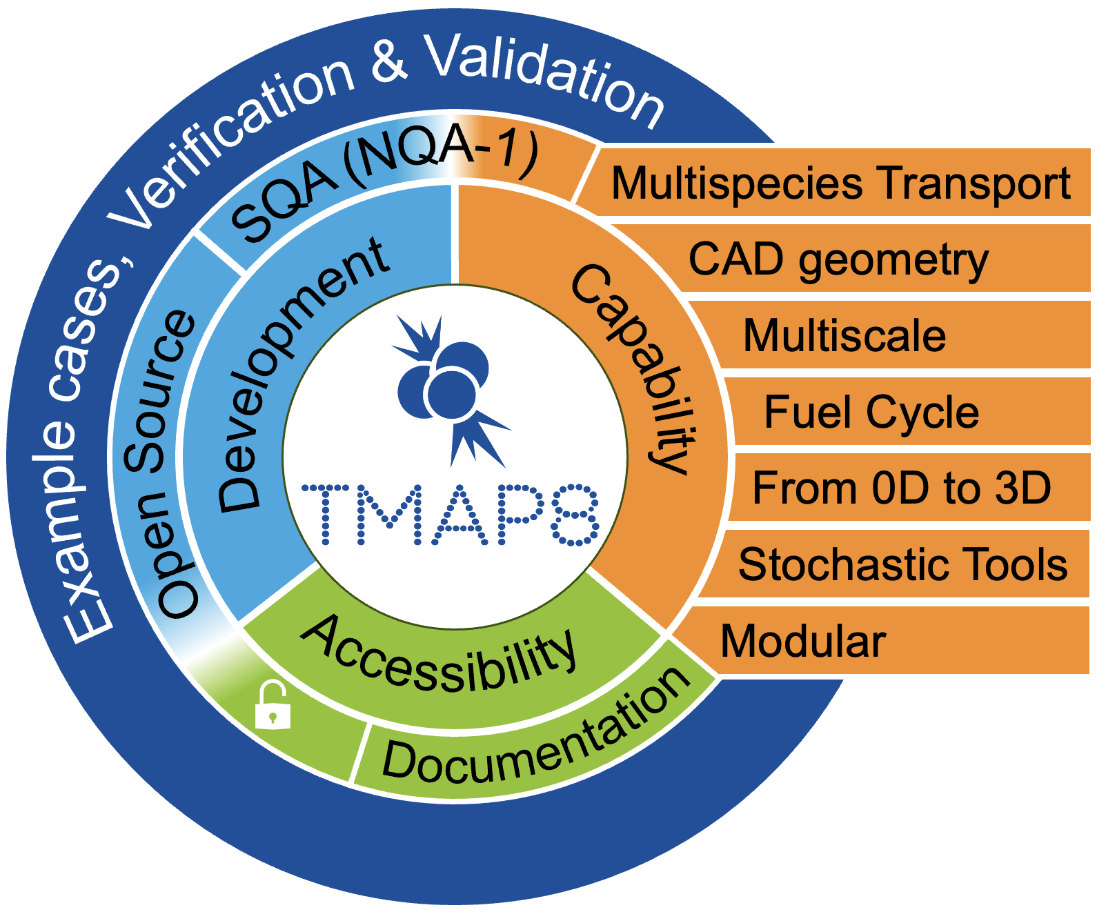
The TMAP4/7 capabilities and physics are available in TMAP8.
TMAP4 and TMAP7, although widely used, have limitations that TMAP8 overcomes.
TMAP8 enables high fidelity, multi-scale, 0D to 3D, multispecies, multiphysics simulations of tritium transport, and offers massively parallel capabilities.
TMAP8 is open source, Nuclear Quality Assurance level 1 (NQA-1) compliant, offers user support and a licensing approach (LGPL-2.1) selected for collaboration.
TMAP8 Theory
TMAP8's documentation provides a theory manual to describe the base theory used in TMAP8, focused in particular on different approaches available to model surface reactions.
However, this list is not exhaustive, and for a more comprehensive description of capabilities, theoretical concepts, and available objects, refer to:
the publications listed in the List of Publications using TMAP8
the Complete TMAP8 Input File Syntax page.
For the derivation of the weak form of the tritium transport system of equations in solids, refer to the appendix of this TMAP8 publication.
TMAP8 key capabilities - fuel cycle
TMAP8 is able to perform fuel cycle calculations at the system scale.
It has been benchmarked against the fuel cycle model described by Abdou et al. (2021), and the model described in Meschini et al. (2023).
Ongoing efforts are using the MultiApp system to concurrently perform component-level calculations and use the results in fuel cycle calculations to accurately model the tritium fuel cycle.
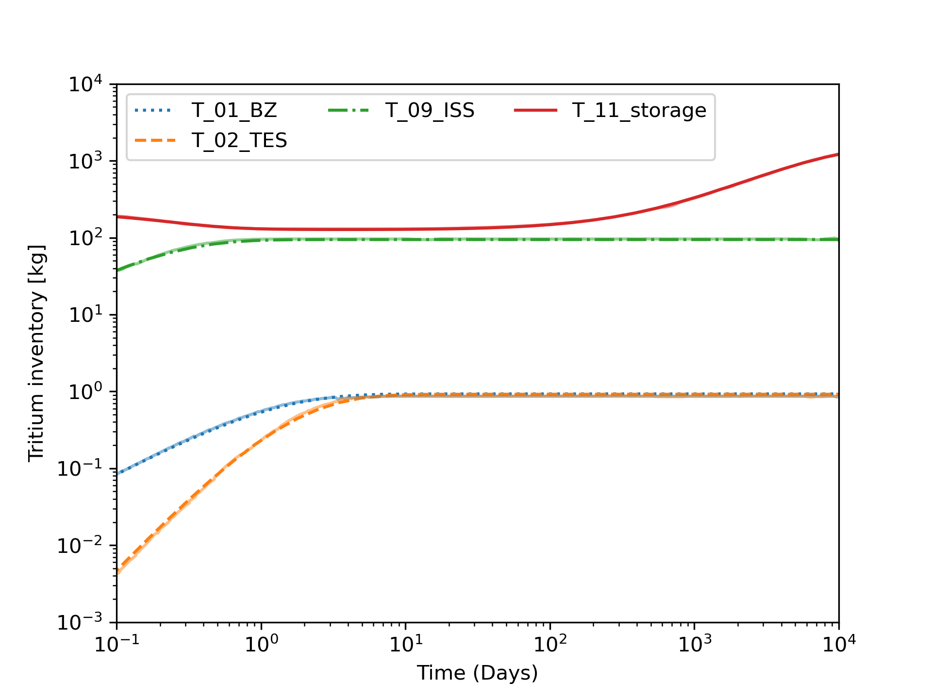
Figure from the fuel cycle example from Abdou et al.
TMAP8 key capabilities - Stochastic tools
The integration of the stochastic tools module in TMAP8 supports key capabilities:
Model calibration
Experimental analysis
Uncertainty quantification
Error identification (experimental uncertainty vs. model inadequacy vs. parameter uncertainty)
Sensitivity analysis
Surrogate model development
etc.
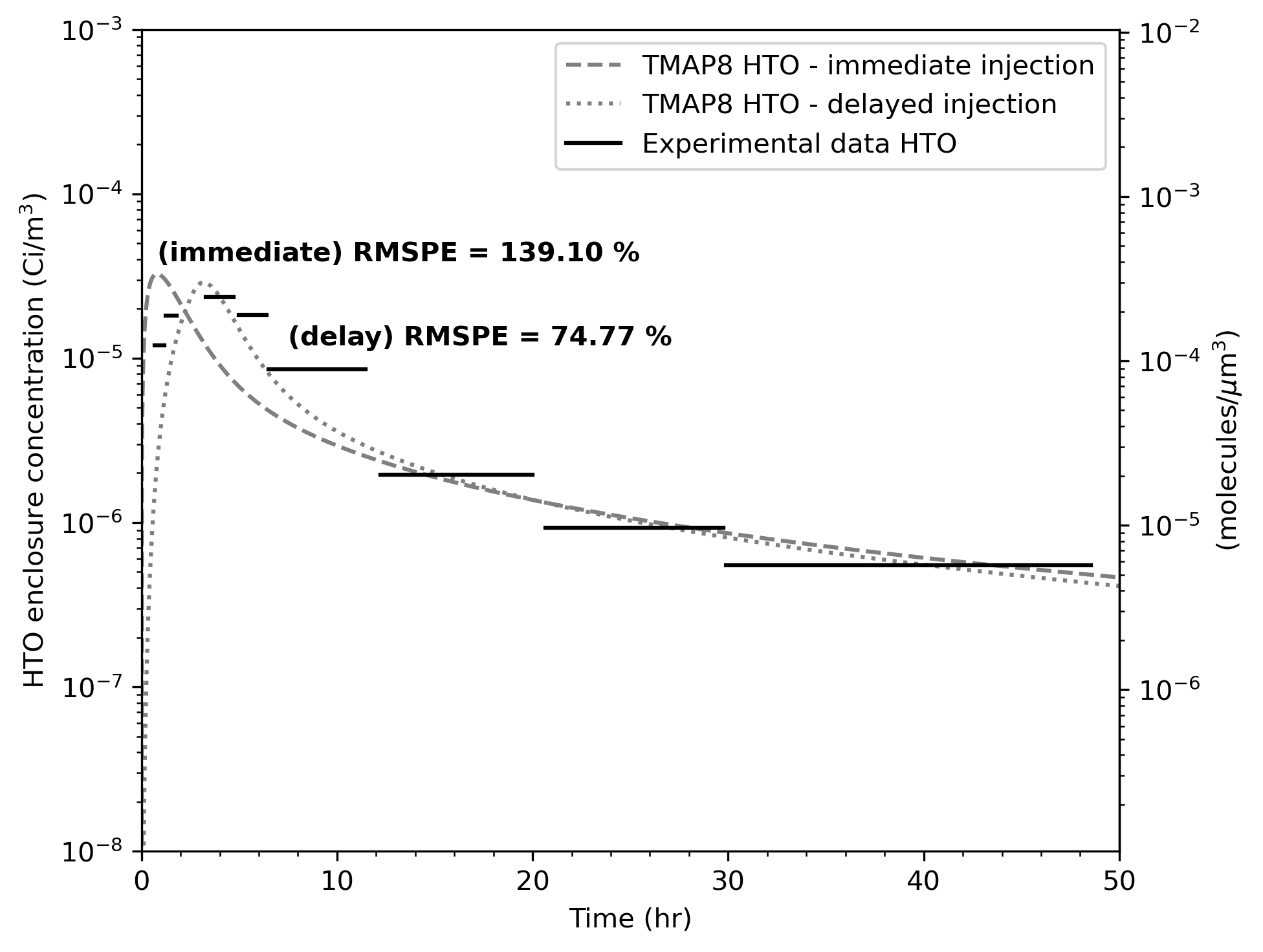
Figure from the val-2c validation case calibration.
TMAP8 key capabilities
pore-scale transport
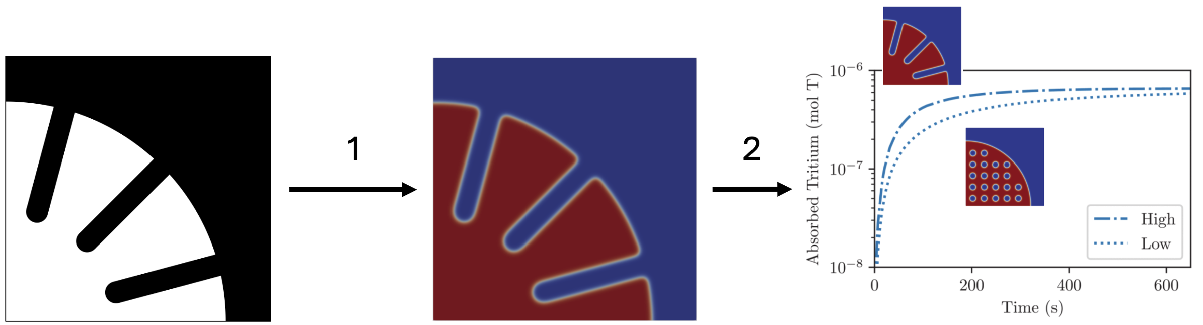
Figure from the pore-scale tritium transport example.
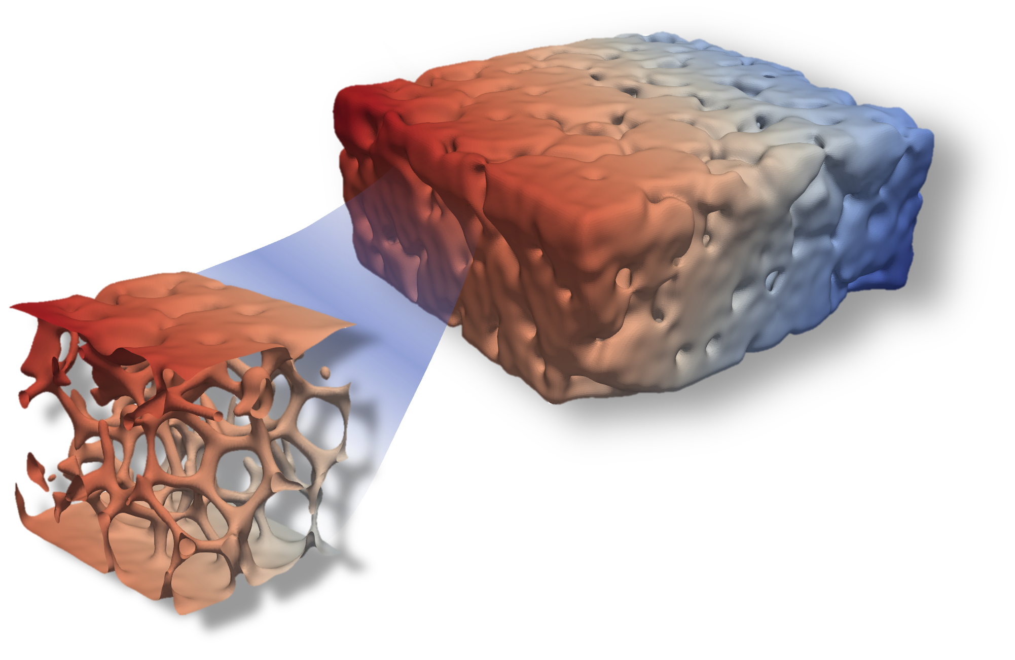
Thanks to the ImageFunction and phase-field module capabilities, TMAP8 can perform mesoscale simulations of tritium transport.
It can use sequential images of real or generated microstructures and perform tritium transport on them.
This capability is detailed in the pore-scale tritium transport example.
TMAP8 Verification & Validation (V&V)
Verification is the process of ensuring that a computational model accurately represents the underlying mathematical model and its solution. Verification can be satisfied by comparing modeling predictions against analytical solutions for simple cases, or leveraging the method of manufactured solutions (MMS), which is supported in MOOSE.
Validation, on the other hand, is the process of determining the extent to which a model accurately represents the real world for its intended uses, which requires comparison against experimental data.
TMAP8's V&V case suite now surpasses TMAP4's and TMAP7's, and continues to grow. It is a resource for users wanting to learn more about TMAP8's accuracy, and for users wanting to use them as starting point for their simulations.
Check out the TMAP8 V&V cases and all relevant input files and documentation on the:
Later in the hands on part of this workshop, we will go through some V&V cases in more detail.
TMAP8 Examples
TMAP8's example cases list simulations performed with TMAP8 that highlight specific capabilities. The example cases differ from the V&V cases in that they do not necessarily have analytical solutions or experimental data to be compared against. In geenral, the example cases also describe how the input file relates to the simulation, making them great resources for users. Hence, these cases can serve as additional tutorial cases, or as starting point for new simulations.
Check out the TMAP8 example cases and all relevant input file and documentation on the:
It includes examples for fuel cycle calculations, divertor monoblock modeling, and pore microstructure modeling.
Summary
TMAP8 Verification Walkthrough:
Tritium Permeation and Trapping
From Simple Diffusion to Multi-trap Systems
Overview
Purpose: Modeling tritium transport with progressing complexity.
ver-1dd: Pure diffusion without trapping (Documentation)
ver-1d: Diffusion with single trap type (Documentation)
ver-1dc: Diffusion with multiple trap types (Documentation)
Based on established literature resources from the TMAP4 and TMAP7 eras:
Expanded upon & updated in Simon et al. (2025)
Demonstrates TMAP8's capability to handle increasingly complex tritium transport scenarios.
Physical Problem: Permeation Through a Membrane
Configuration
1D slab geometry
Constant source at upstream side ( m)
Permeation flux measured at downstream side ( m)
Breakthrough time characterizes transport
Key Parameters
Diffusivity: /s
Temperature: K
Upstream concentration: atom fraction
Slab thickness: m
Understanding MOOSE Input File Structure
Basic Anatomy of a TMAP8 Input File
[Block]
  [subblock]
    type = MyObject
    parameter1 = value1
    parameter2 = value2
  []
[]
Key Sections We'll Explore
[Mesh]- Define geometry[Variables]- Declare unknowns to solve for[Kernels]- Define physics equations[BCs]- Define boundary conditions[Executioner]- Define the solution method[Outputs]- Setup how results should be saved
Case 1: Pure Diffusion (ver-1dd)
Governing Equation
Simplest case: Fickian diffusion only
No trapping mechanisms
Baseline for comparison with trap-inclusive models
Analytical solution available for verification
Case 1: Input File Structure - Mesh and Variables
[Mesh]
  type = GeneratedMesh
  dim = 1
  nx = ${nx_num}
  xmax = 1
[]

[Variables]
  [mobile]
  []
[]
1D mesh with 200 elements and a maximum length of 1 m.
nx_numis defined as 200 at the top of the file, and${}syntax is used to utilize it elsewhere.xminin aMeshobject generally defaults to 0.
Single variable
mobilefor the mobile species concentrationStarts with zero initial concentration (not giving an
ICsblock and not settinginitial_conditionin this sub-block defaults to zero).
Case 1: Input File Structure -
Physics Implementation
[Kernels]
  [diff]
    type = Diffusion
    variable = mobile
  []
  [time]
    type = TimeDerivative
    variable = mobile
  []
[]
Diffusionkernel:where m/s.
TimeDerivativekernel:Together, they form the diffusion equation that we are aiming to solve.
Case 1: Input File Structure -
Boundary Conditions
[BCs]
  [left]
    type = DirichletBC
    variable = mobile
    value = '${fparse cl / cl}'
    boundary = left
  []
  [right]
    type = DirichletBC
    variable = mobile
    value = 0
    boundary = right
  []
[]
A constant source of
value = 1is placed at left (upstream), due to normalizing the concentration (cl = 3.1622e18atoms/).Note the use of the
fparsesystem to perform this simple calculation.In this case, the action of calculating the source is simple, but use of the parsing system can, in general, enhance readability of the input file.
A concentration of zero is set at right (downstream).
Case 1: Input File Structure -
Postprocessors
[Postprocessors]
  [outflux]
    type = SideDiffusiveFluxAverage
    boundary = 'right'
    diffusivity = ${diffusivity}
    variable = mobile
  []
  [scaled_outflux]
    type = ScalePostprocessor
    value = outflux
    scaling_factor = ${cl}
  []
[]
Here, postprocessors are used to calculate two quantities:
The raw outward flux average on the downstream boundary using the SideDiffusiveFluxAverage object, given the
diffusivityfrom the top of the input.The raw outward flux average is then scaled to its actual value using the ScalePostprocessor, which takes the
outfluxvalue and scales it by the concentrationcl.
Case 1: Input File Structure -
Preconditioning and Solving
[Preconditioning]
  [smp]
    type = SMP
    full = true
  []
[]

[Executioner]
  type = Transient
  end_time = ${simulation_time}
  dt = ${interval_time}
  dtmin = ${interval_time_min}
  solve_type = NEWTON
  scheme = BDF2
  nl_abs_tol = 1e-13
  petsc_options_iname = '-pc_type'
  petsc_options_value = 'lu'
  automatic_scaling = true
  verbose = true
  compute_scaling_once = false
[]
For preconditioning, we have a SMP (Single Matrix Preconditioner).
SMP builds a preconditioning matrix using user-defined off-diagonal parts of the Jacobian matrix.
Use of
full = trueuses all of the off-diagonal blocks, but tuning of the preconditioning can allow focus on one or more physics in your system.
Given the time derivative term, we use a Transient executioner with a Newton solver.
Other solver parameters - including total simulation time, the timestep, and the minimum timestep allowed - is set using parser syntax.
Case 1: Input File Structure - Outputs
[Outputs]
  exodus = true
  csv = true
  [dof]
    type = DOFMap
    execute_on = initial
  []
  perf_graph = true
[]
Here, we want both Exodus and CSV output. By simply setting:
exodus = true
csv = true
We also turn on DOFMap, only executing it on the initial timestep (after the matrix is constructed). This provides output information on how the matrix is constructed, which is helpful for complicated models.
Finally, we turn on a simple performance table in the Console output.
Case 1: Let's Run It!
If using a cloned and locally-built copy of TMAP8:
cd test/tests/ver-1dd/
../../../tmap8-opt -i ver-1dd.i
If using a Docker container:
cd /tmap8-workdir/tmap8/ver-1dd
tmap8-opt -i ver-1dd.i
The output can then be visualized using ParaView, or by using the comparison_ver-1dd.py script with some light modifications (change the location of the data file to the output you just generated).
What to Look For
Convergence messages in terminal
Exodus output files with field data (.e extension)
CSV files with Postprocessor data
Case 1: Verification Results
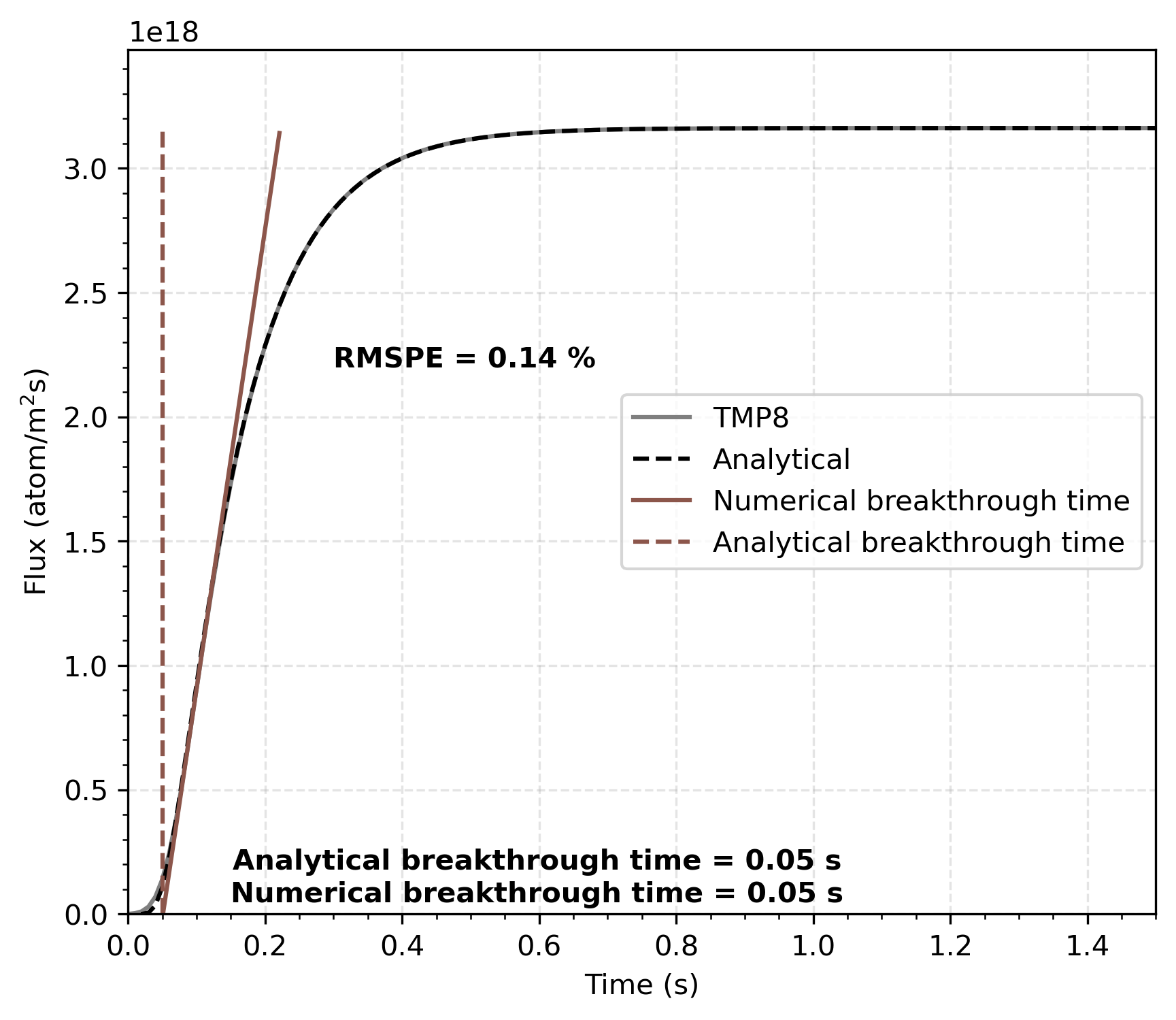
Breakthrough time: seconds (both analytical and TMAP8)
Excellent agreement throughout transient
Case 2: Single Trap Type (ver-1d)
In this case, we are modeling permeation through a membrane with a constant source in which traps are operative.
Traps correspond to physical places in materials where tritium atoms can get trapped, and therefore slow down transport. For example, tritium atoms can be trapped in interstitial sites, vacancies, dislocations, grain boundaries, pores, etc., which can all be included as traps in the model. These trapping sites are described with an associated density (which can evolve as a function of space, time, irradiation, etc.) and rates and energies for trapping and release.
In the current case, we account for one type of trapping site. The following case will introduce a total of three trapping types. Note that TMAP8 can incorporate an arbitrary number of trapping sites.
Case 2: Single Trap Type (ver-1d)
We solve the following equations:
For mobile species:
For trapped species:
For empty trapping sites:
where:
and are the concentrations of the mobile and trapped species respectively
is the diffusivity of the mobile species
and are the trapping and release rate coefficients
is a factor converting the magnitude of to be closer to for better numerical convergence
is the fraction of host sites that can contribute to trapping
is the concentration of empty trapping sites
is the host density.
Trapping parameter
The breakthrough time may have one of two limiting values depending on whether the trapping is in the effective diffusivity or strong-trapping regimes. A trapping parameter is defined by:
where:
= lattice parameter
= Debye frequency ( )
= trapping site fraction
= diffusivity pre-exponential
= diffusion activation energy
= trap energy
= Boltzmann's constant
= temperature
= dissolved gas atom fraction
Effective Diffusivity Regime
The discriminant for which regime is dominant is the ratio of to c/. If c/, then the effective diffusivity regime applies, and the permeation transient is identical to the standard diffusion transient, with the diffusivity replaced by an effective diffusivity
to account for the fact that trapping leads to slower transport.
In this limit, the breakthrough time, defined as the intersection of the steepest tangent to the diffusion transient with the time axis, will be
where is the thickness of the slab and D is the diffusivity of the gas through the material.
Strong-trapping Regime
In the deep-trapping limit, c/, and no permeation occurs until essentially all the traps have been filled. Then the system quickly reaches steady-state. The breakthrough time is given by
where is the steady dissolved gas concentration at the upstream (x = 0) side.
Case Description
In this scenario, examine reach regime using two input files:
ver-1d-diffusion.i: where diffusion is the rate-limiting step
ver-1d-trapping.i: where trapping is the rate-limiting step.
This is the same domain configuration as in Case 1.
Key Parameters
Diffusivity: m/s
Temperature: K
Upstream concentration: atom fraction
Slab thickness: m
Trapping site fraction: 10 (0.1)
Lattice parameter: m
(Diffusion), (Trapping)
Trapping rate coefficient: 1/s
Release rate coefficient: 1/s
Host density: atoms / m
Case 2: Diffusion Limit Input File - Variables
In this case, we'll be highlighting the main changes from Case 1, where we only had diffusion for a single mobile species.
[Variables]
  [mobile]
  []
  [trapped]
  []
[]
Now, we have two species,
trappedandmobile. Similar to Case 1, themobilevariable is our primary variable, as we'll plot the downstream flux for comparison to analytical solutions.Both use the default initial concentrations of zero, as well as the default FEM families/order.
A Note on ReferenceResidualProblem
The ReferenceResidualProblem MOOSE Problem type is designed to allow custom criteria for convergence for separate, coupled physics by using tagged vectors to designate portions of the system matrix.
These tags are set in the
[Problem]block usingreference vectorandextra_tag_vectorsand then used in the *Kernel blocks (of all types).
[Problem]
  type = ReferenceResidualProblem
  extra_tag_vectors = 'ref'
  reference_vector = 'ref'
[]
[Kernels]
  [diff]
    type = Diffusion
    variable = mobile
    extra_vector_tags = ref
  []
[]
Case 2: Diffusion Limit Input File - Coupling Mobile and Trapped
[Kernels]
  [diff]
    type = Diffusion
    variable = mobile
    extra_vector_tags = ref
  []
  [time]
    type = TimeDerivative
    variable = mobile
    extra_vector_tags = ref
  []
  [coupled_time]
    type = CoupledTimeDerivative
    variable = mobile
    v = trapped
    extra_vector_tags = ref
  []
[]
We now have a new Kernel in the PDE corresponding to
mobile:represented by CoupledTimeDerivative.
Note that "v" is a common parameter name representing the coupled variable in many MOOSE objects.
Case 2: Diffusion Limit Input File - Trapped Physics
[NodalKernels]
  [time]
    type = TimeDerivativeNodalKernel
    variable = trapped
  []
  [trapping]
    type = TrappingNodalKernel
    variable = trapped
    alpha_t = 1e15
    N = '${fparse 3.1622e22 / cl}'
    Ct0 = 0.1
    mobile_concentration = 'mobile'
    temperature = ${temperature}
    extra_vector_tags = ref
  []
  [release]
    type = ReleasingNodalKernel
    alpha_r = 1e13
    temperature = ${temperature}
    detrapping_energy = 100
    variable = trapped
  []
[]
To represent the trapping physics on the nodes, we can use the NodalKernels System.
TimeDerivativeNodalKernel is used for:
TrappingNodalKernel is used for:
Finally, ReleasingNodalKernel is used for:
Case 2: Diffusion Limit Input File - Executioner
[Executioner]
  type = Transient
  end_time = 3
  dt = .01
  dtmin = .01
  solve_type = NEWTON
  petsc_options_iname = '-pc_type'
  petsc_options_value = 'lu'
  automatic_scaling = true
  verbose = true
  compute_scaling_once = false
[]
The executioner in this case is similar to that in Case 1.
Note that a different TimeStepper System is used (the default,
implicit-euler).The absolute non-linear tolerance is also using the smaller default value (
1e-50).
Case 2: Strong Trapping Input File -
AuxVariables and AuxKernels
For the deep trapping limit case, we'll cover the additions of objects to determine the empty trapping site concentration.
[AuxVariables]
  [empty_sites]
  []
  [scaled_empty_sites]
  []
  [trapped_sites]
  []
  [total_sites]
  []
[]

[AuxKernels]
  [empty_sites]
    variable = empty_sites
    type = EmptySitesAux
    N = '${fparse N / cl}'
    Ct0 = .1
    trap_per_free = ${trap_per_free}
    trapped_concentration_variables = trapped
  []
  [scaled_empty]
    variable = scaled_empty_sites
    type = NormalizationAux
    normal_factor = ${cl}
    source_variable = empty_sites
  []
  [trapped_sites]
    variable = trapped_sites
    type = NormalizationAux
    normal_factor = ${trap_per_free}
    source_variable = trapped
  []
  [total_sites]
    variable = total_sites
    type = ParsedAux
    expression = 'trapped_sites + empty_sites'
    coupled_variables = 'trapped_sites empty_sites'
  []
[]
Because the empty trapping concentration is not a differential equation, we can solve for it using the AuxKernels System:
AuxKernels are also used (in the case of
scaled_emptyandtrapped_sites) to calculate the total concentration of trapping sites in the model.
Case 2: Numerical Considerations
The trapping test input file can generate oscillations in the solution due to the feedback loop between the diffusion PDE and trap evolution ODE. Two strategies are used:
Finer Mesh and Time Step
[Mesh]
  type = GeneratedMesh
  dim = 1
  nx = 1000
  xmax = 1
[]

[Executioner]
  [TimeStepper]
    type = IterationAdaptiveDT
    dt = 1e-6
    optimal_iterations = 9
    growth_factor = 1.1
    cutback_factor = 0.909
  []
[]
Ramped Boundary Condition
[BCs]
  [left]
    type = FunctionDirichletBC
    variable = mobile
    function = 'BC_func'
    boundary = left
  []
[]

[Functions]
  [BC_func]
    type = ParsedFunction
    expression = '${fparse cl / cl}*tanh( 3 * t )'
  []
[]
Case 2: Trapping Parameter Study
As a reminder, the trapping parameter is the key discriminant to which regime is dominating.
Effective Diffusivity
Regime
When c/
Set:
c/
Strong-Trapping Regime / Deep Trapping Limit
When c/
Set
c/
Case 2: Diffusion-Limited Results
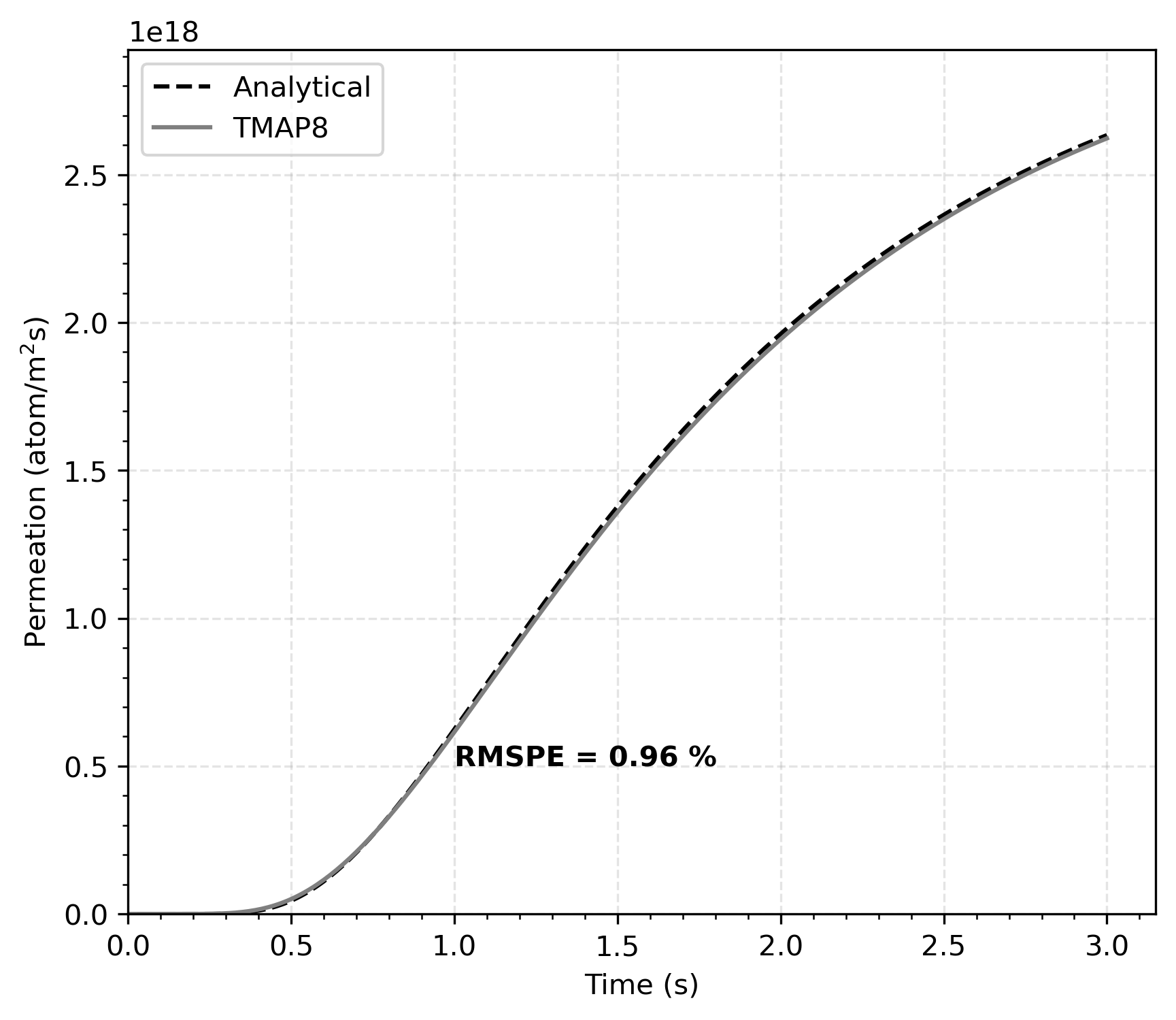
Trapping slows but doesn't stop diffusion
Smooth permeation curve
Case 2: Trap-Limited Results
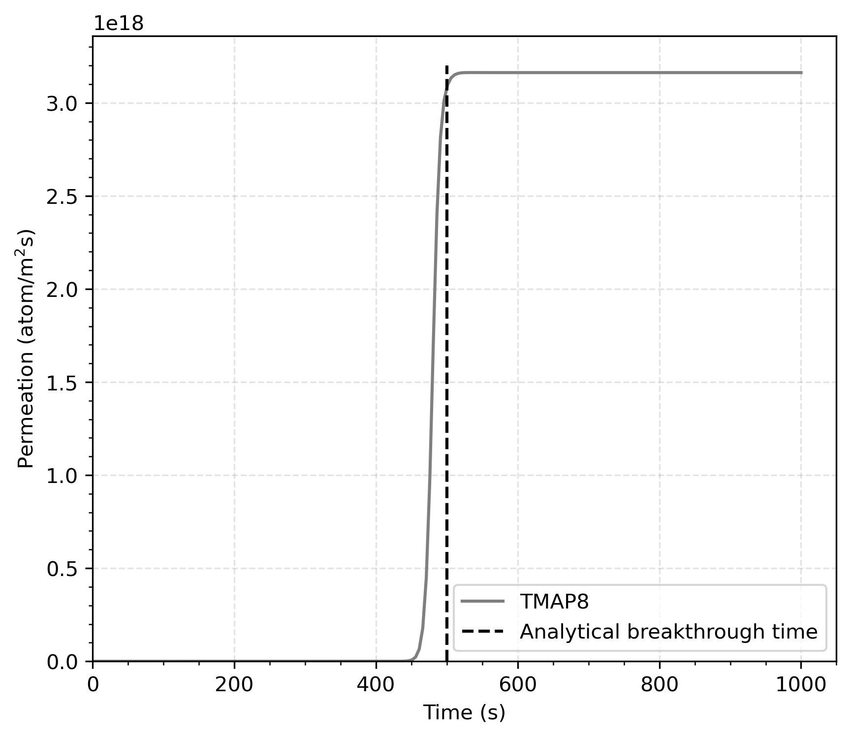
Must fill traps before significant permeation
Sharp transition at breakthrough
Case 3: Multiple Trap Types (ver-1dc)
Extended System of Equations
This case is very similar to Case 2, except there are now three different types of traps.
Mobile species with three trap interactions:
Each trap evolves independently (i = 1, 2, 3). Finally, for the empty trapping sites:
Case 3: Base Input File Strategy
This case introduces the "input file include" capability in practice.
ver-1dc_base.icontains the mesh, Problem, Variables, Kernels, NodalKernels, Preconditioning, and Executioner settings for both the standard and MMS input files.This is done to enable multiple input files to use the same common elements.
This modular design:
Eases maintainability and repeatability
Reduces redundancy and errors
Allows for case-specific input files
Enables more readable highlight of unique physics
Case 3: Base Input File
# This is the base input file for the ver-1dc case.
# This input file is meant to be included within both the ver-1dc.i
# and ver-1dc_mms.i input files to be complete.
# Its purpose is to centralize the capability common to the two cases
# within one file to minimize redundancy and ease maintenance.
# It is not meant to be run on its own.

epsilon_1 = ${units 100 K}
epsilon_2 = ${units 500 K}
epsilon_3 = ${units 800 K}
temperature = ${units 1000 K}
trapping_site_fraction_1 = 0.10 # (-)
trapping_site_fraction_2 = 0.15 # (-)
trapping_site_fraction_3 = 0.20 # (-)
diffusivity = 1 # m^2/s

[Mesh]
  type = GeneratedMesh
  dim = 1
  nx = ${nx_num}
  xmax = 1
[]

[Problem]
  type = ReferenceResidualProblem
  extra_tag_vectors = 'ref'
  reference_vector = 'ref'
[]

[Variables]
  [mobile]
  []
  [trapped_1]
  []
  [trapped_2]
  []
  [trapped_3]
  []
[]

[Kernels]
  [diff]
    type = Diffusion
    variable = mobile
    extra_vector_tags = ref
  []
  [time]
    type = TimeDerivative
    variable = mobile
    extra_vector_tags = ref
  []
  [coupled_time_1]
    type = CoupledTimeDerivative
    variable = mobile
    v = trapped_1
    extra_vector_tags = ref
  []
  [coupled_time_2]
    type = CoupledTimeDerivative
    variable = mobile
    v = trapped_2
    extra_vector_tags = ref
  []
  [coupled_time_3]
    type = CoupledTimeDerivative
    variable = mobile
    v = trapped_3
    extra_vector_tags = ref
  []
[]

[NodalKernels]
  # For first traps
  [time_1]
    type = TimeDerivativeNodalKernel
    variable = trapped_1
  []
  [trapping_1]
    type = TrappingNodalKernel
    variable = trapped_1
    alpha_t = '${trapping_rate_coefficient}'
    N = '${fparse N / cl}'
    Ct0 = '${trapping_site_fraction_1}'
    mobile_concentration = 'mobile'
    temperature = '${temperature}'
    extra_vector_tags = ref
  []
  [release_1]
    type = ReleasingNodalKernel
    alpha_r = '${release_rate_coefficient}'
    temperature = '${temperature}'
    detrapping_energy = '${epsilon_1}'
    variable = trapped_1
  []
  # For second traps
  [time_2]
    type = TimeDerivativeNodalKernel
    variable = trapped_2
  []
  [trapping_2]
    type = TrappingNodalKernel
    variable = trapped_2
    alpha_t = '${trapping_rate_coefficient}'
    N = '${fparse N / cl}'
    Ct0 = '${trapping_site_fraction_2}'
    mobile_concentration = 'mobile'
    temperature = '${temperature}'
    extra_vector_tags = ref
  []
  [release_2]
    type = ReleasingNodalKernel
    alpha_r = '${release_rate_coefficient}'
    temperature = '${temperature}'
    detrapping_energy = '${epsilon_2}'
    variable = trapped_2
  []
  # For third traps
  [time_3]
    type = TimeDerivativeNodalKernel
    variable = trapped_3
  []
  [trapping_3]
    type = TrappingNodalKernel
    variable = trapped_3
    alpha_t = '${trapping_rate_coefficient}'
    N = '${fparse N / cl}'
    Ct0 = '${trapping_site_fraction_3}'
    mobile_concentration = 'mobile'
    temperature = '${temperature}'
    extra_vector_tags = ref
  []
  [release_3]
    type = ReleasingNodalKernel
    alpha_r = '${release_rate_coefficient}'
    temperature = '${temperature}'
    detrapping_energy = '${epsilon_3}'
    variable = trapped_3
  []
[]

[Preconditioning]
  [smp]
    type = SMP
    full = true
  []
[]

[Executioner]
  type = Transient
  end_time = ${simulation_time}
  dtmax = ${time_interval_max}
  solve_type = NEWTON
  scheme = ${scheme}
  petsc_options_iname = '-pc_type'
  petsc_options_value = 'lu'
  line_search = 'none'
[]
Case 3: Defining Multiple Traps
Multiple sites can have different properties through the use of separate sets of NodalKernels to represent the unique properties of each trap.
For example, for trapped_1:
[NodalKernels]
  [time_1]
    type = TimeDerivativeNodalKernel
    variable = trapped_1
  []

  [trapping_1]
    type = TrappingNodalKernel
    variable = trapped_1
    alpha_t = '${trapping_rate_coefficient}'
    N = '${fparse N / cl}'
    Ct0 = '${trapping_site_fraction_1}'
    mobile_concentration = 'mobile'
    temperature = '${temperature}'
    extra_vector_tags = ref
  []

  [release_1]
    type = ReleasingNodalKernel
    alpha_r = '${release_rate_coefficient}'
    temperature = '${temperature}'
    detrapping_energy = '${epsilon_1}'
    variable = trapped_1
  []
[]
Each Trap Gets:
Its own solution variable
Independent evolution equation
Unique parameters (site fraction, energy)
Case 3: Three Trap Parameters
Three traps that are relatively weak are assumed to be active in the slab. Other parameters are the same as the trap in the effective diffusivity limit in ver-1d.
Trap Type 1
Trapping site fraction: 0.1
= 100 K
Trap Type 2
Trapping site fraction: 0.15
= 500 K
Trap Type 3
Trapping site fraction: 0.2
= 800 K
Case 3: Verification Results
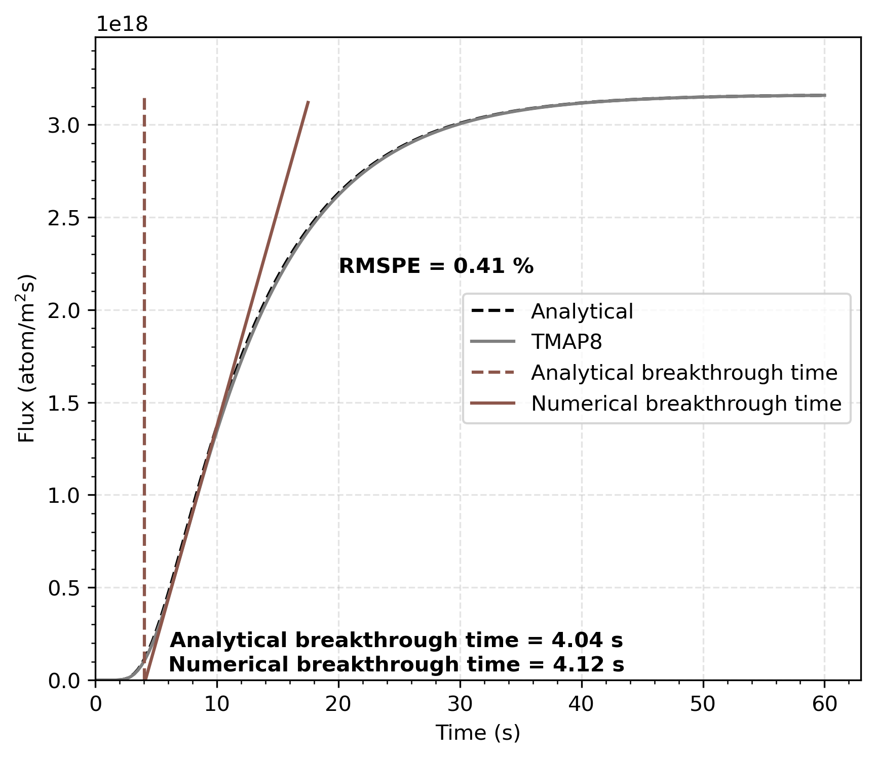
Breakthrough time: 4.04 s (analytical) vs 4.12 s (TMAP8)
Combined effect of all three traps
Case 3: MMS Verification Approach
A detailed and step-by-step description of the method of manufactured solutions (MMS) approach is available on the MOOSE MMS page. The ver-1dc documentation page provides more information about how to apply the MMS approach to this case.
The main steps of the MMS approach are:
select spatial smoothly-varying sinusoidal spatial solutions for the mobile and trapped species.
input them in the desired equations and derive the forcing functions.
re-write the equations to include the forcing function such that the solution for the modified system is that selected above.
solve these equations, comparing the calculated solutions against the selected solutions for each species.
Case 3: MMS Verification Approach (continued)
Exact solutions and forcing functions:
[exact_u]
  type = ParsedFunction
  expression = 't*cos(x)'
[]
[forcing_u]
  type = ParsedFunction
  expression = '(1/2)*N*frac1*cos(x) + (1/2)*N*frac2*cos(x) + (1/2)*N*frac3*cos(x) + D*t*cos(x) + cos(x)'
  symbol_names = 'N frac1 frac2 frac3 D'
  symbol_values = '${N} ${frac1} ${frac2} ${frac3} ${diffusivity}'
[]
[exact_t1]
  type = ParsedFunction
  expression = '(1/2)*N*frac1*(t*cos(x) + 1)'
  symbol_names = 'frac1 N'
  symbol_values = '${frac1} ${N}'
[]
[forcing_t1]
  type = ParsedFunction
  expression = '(1/2)*frac1*(N*cos(x) + alphar*N*(t*cos(x) + 1)*exp(-epsilon_1/temperature) - alphat*t*(-t*cos(x) + 1)*cos(x))'
  symbol_names = 'alphar alphat N frac1 temperature epsilon_1'
  symbol_values = '${alphar} ${alphat} ${N} ${frac1} ${temperature} ${epsilon_1}'
[]
[exact_t2]
  type = ParsedFunction
  expression = '(1/2)*N*frac2*(t*cos(x) + 1)'
  symbol_names = 'frac2 N'
  symbol_values = '${frac2} ${N}'
[]
[forcing_t2]
  type = ParsedFunction
  expression = '(1/2)*frac2*(N*cos(x) + alphar*N*(t*cos(x) + 1)*exp(-epsilon_2/temperature) - alphat*t*(-t*cos(x) + 1)*cos(x))'
  symbol_names = 'alphar alphat N frac2 temperature epsilon_2'
  symbol_values = '${alphar} ${alphat} ${N} ${frac2} ${temperature} ${epsilon_2}'
[]
[exact_t3]
  type = ParsedFunction
  expression = '(1/2)*N*frac3*(t*cos(x) + 1)'
  symbol_names = 'frac3 N'
  symbol_values = '${frac3} ${N}'
[]
[forcing_t3]
  type = ParsedFunction
  expression = '(1/2)*frac3*(N*cos(x) + alphar*N*(t*cos(x) + 1)*exp(-epsilon_3/temperature) - alphat*t*(-t*cos(x) + 1)*cos(x))'
  symbol_names = 'alphar alphat N frac3 temperature epsilon_3'
  symbol_values = '${alphar} ${alphat} ${N} ${frac3} ${temperature} ${epsilon_3}'
[]
Case 3: MMS Verification Approach (continued)
Application of functions to Kernels/NodalKernels/BCs to "force" exact solution:
[Kernels]
  [diff]
    type = Diffusion
    variable = mobile
    extra_vector_tags = ref
  []
  [time]
    type = TimeDerivative
    variable = mobile
    extra_vector_tags = ref
  []
  [coupled_time_1]
    type = CoupledTimeDerivative
    variable = mobile
    v = trapped_1
    extra_vector_tags = ref
  []
  [coupled_time_2]
    type = CoupledTimeDerivative
    variable = mobile
    v = trapped_2
    extra_vector_tags = ref
  []
  [coupled_time_3]
    type = CoupledTimeDerivative
    variable = mobile
    v = trapped_3
    extra_vector_tags = ref
  []

  [forcing]
    type = BodyForce
    variable = mobile
    function = 'forcing_u'
  []
[]

[NodalKernels]
  # For first traps
  [time_1]
    type = TimeDerivativeNodalKernel
    variable = trapped_1
  []
  [trapping_1]
    type = TrappingNodalKernel
    variable = trapped_1
    alpha_t = '${trapping_rate_coefficient}'
    N = '${fparse N / cl}'
    Ct0 = '${trapping_site_fraction_1}'
    mobile_concentration = 'mobile'
    temperature = '${temperature}'
    extra_vector_tags = ref
  []
  [release_1]
    type = ReleasingNodalKernel
    alpha_r = '${release_rate_coefficient}'
    temperature = '${temperature}'
    detrapping_energy = '${epsilon_1}'
    variable = trapped_1
  []
  # For second traps
  [time_2]
    type = TimeDerivativeNodalKernel
    variable = trapped_2
  []
  [trapping_2]
    type = TrappingNodalKernel
    variable = trapped_2
    alpha_t = '${trapping_rate_coefficient}'
    N = '${fparse N / cl}'
    Ct0 = '${trapping_site_fraction_2}'
    mobile_concentration = 'mobile'
    temperature = '${temperature}'
    extra_vector_tags = ref
  []
  [release_2]
    type = ReleasingNodalKernel
    alpha_r = '${release_rate_coefficient}'
    temperature = '${temperature}'
    detrapping_energy = '${epsilon_2}'
    variable = trapped_2
  []
  # For third traps
  [time_3]
    type = TimeDerivativeNodalKernel
    variable = trapped_3
  []
  [trapping_3]
    type = TrappingNodalKernel
    variable = trapped_3
    alpha_t = '${trapping_rate_coefficient}'
    N = '${fparse N / cl}'
    Ct0 = '${trapping_site_fraction_3}'
    mobile_concentration = 'mobile'
    temperature = '${temperature}'
    extra_vector_tags = ref
  []
  [release_3]
    type = ReleasingNodalKernel
    alpha_r = '${release_rate_coefficient}'
    temperature = '${temperature}'
    detrapping_energy = '${epsilon_3}'
    variable = trapped_3
  []

  [forcing_1]
    type = UserForcingFunctionNodalKernel
    variable = trapped_1
    function = forcing_t1
  []
  [forcing_2]
    type = UserForcingFunctionNodalKernel
    variable = trapped_2
    function = forcing_t2
  []
  [forcing_3]
    type = UserForcingFunctionNodalKernel
    variable = trapped_3
    function = forcing_t3
  []
[]

[BCs]
  [dirichlet]
    type = FunctionDirichletBC
    variable = mobile
    function = 'exact_u'
    boundary = 'left right'
  []
[]
Case 3: MMS Spatial Convergence
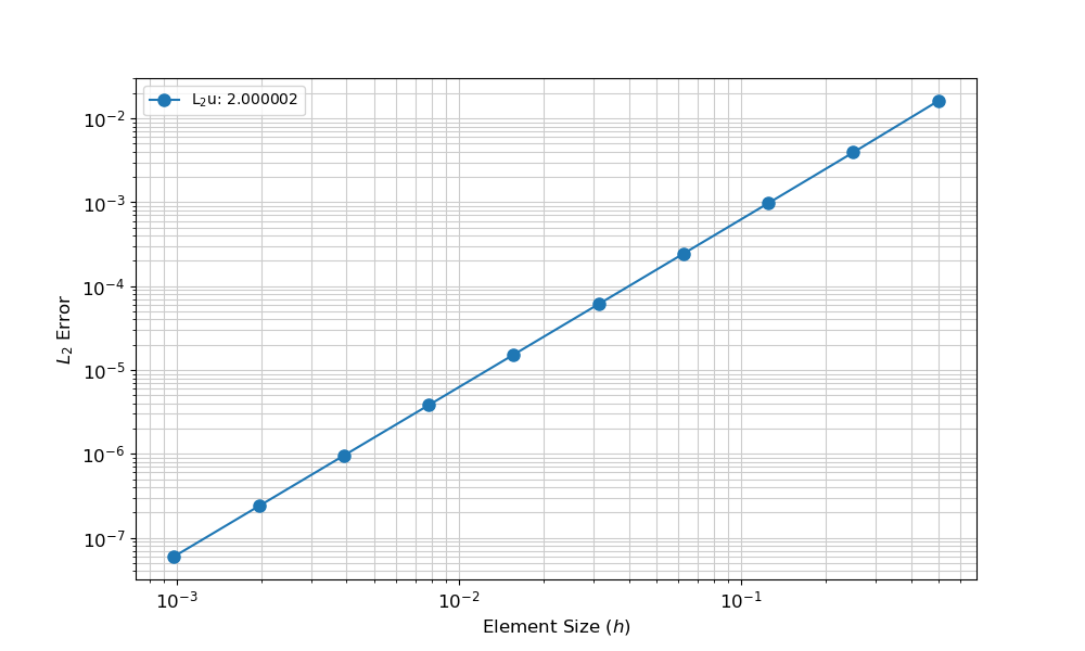
10 levels of mesh refinement
Confirms proper implementation
Quadratic convergence as expected
Case 1 to 3: effect of trapping on transport
Comparing the three cases below highlights the important effect of trapping sites on tritium transport. All three cases use the same diffusivity for different traps.
Case 1: Diffusion only.
Case 2: One trap,
diffusion-limited regime.
Case 3: three traps,
diffusion-limited regime.
Modifying Input Files - Exercise
Try These Changes to ver-1dd.i:
Change mesh resolution
[Mesh]
  nx = 400  # Was 200
[]
Adjust time stepping
[Executioner]
  dt = 0.0001  # Smaller initial step
[]
Modified diffusivity
[Kernels]
  [diff]
    diffusivity = 0.5  # Slower diffusion
  []
[]
Tips and Tricks
Debug Strategies
Start with coarse mesh, refine gradually
Use simple BCs first, add complexity
Compare with analytical solutions when available
Building Complex Cases
Use a progressive development strategy:
Start Simple: Pure diffusion (ver-1dd)
Add One Trap: Test both regimes (ver-1d)
Multiple Traps: Build incrementally (ver-1dc)
Validate Each Step: Compare with theory
Performance Considerations
Computational Efficiency Tips
[Executioner]
  # For testing - coarse/fast
  nl_abs_tol = 1e-8
  nl_rel_tol = 1e-6

  # For verification - fine/accurate
  nl_abs_tol = 1e-12
  nl_rel_tol = 1e-10
[]

[Mesh]
  # Testing: nx = 100
  # Verification: nx = 1000
[]
Parallel Execution
mpirun -np 4 ~/projects/TMAP8/tmap8-opt -i input.i
Advanced Features in TMAP8
Beyond These Examples
2D/3D Geometries: Change
dimin[Mesh]Multiple Materials: Use
[Materials]blockCoupled Physics: Heat transfer, mechanics
Custom Kernels: Extend with C++
Example: Temp. Dependence Directly in Input
[Materials]
  [diffusivity]
    # (m2/s) tritium diffusivity
    type = DerivativeParsedMaterial
    property_name = 'diffusivity'
    coupled_variables = 'temperature'
    expression = '${tritium_diffusivity_prefactor}*exp(-${tritium_diffusivity_energy}/${ideal_gas_constant}/temperature)'
  []
[]
Key Takeaways
Input File Structure: Hierarchical blocks define physics
Progressive Complexity: Build from simple to complex
Verification Strategy: Compare with analytical solutions
ver-1dd: RMSPE = 0.14%
ver-1d: RMSPE = 0.96%
ver-1dc: RMSPE = 0.41%
Best Practices:
Use base input files for modularity
Start with coarse meshes for development
Validate each physics addition
Document parameter choices
Hands-On Exercise
Your Turn: Modify ver-1d
Open
ver-1d-diffusion.iin your editorChange detrapping energy:
Run the simulation
Compare breakthrough time with original
Questions to Consider:
How does breakthrough time change?
Which regime are we in now?
What value does this correspond to?
Concluding Remarks
By now, participants should:
Understand the purpose and capabilities of MOOSE and TMAP8.
Successfully have installed TMAP8.
Have run and modified simulations, as well as ploted and analyzed results.
Have identified and accessed documentation, tutorials, and community support.
Leave with a clear path for continued use and development.
What is Next? Now that you have completed the workshop, participants can
Check out the other V&V and example cases, run, edit, and analyze them.
Read TMAP8 papers.
Adapt them to your relevant case.
Reach out on the TMAP8 discussion or issue pages with questions, concerns, feedback, or requests.
Discuss collaborations with the TMAP8 developers.
Do you have any feedback on the workshop? Feel free to post if on the TMAP8 discussion or issue pages, or reach out to the TMAP8 developers.
References
- James Ambrosek and Glen R Longhurst. Verification and validation of the tritium transport code TMAP7. Fusion science and technology, 48(1):468–471, 2005.
- James Ambrosek and GR Longhurst. Verification and Validation of TMAP7. Technical Report INEEL/EXT-04-01657, Idaho National Engineering and Environmental Laboratory, December 2008.
- GR Longhurst, SL Harms, ES Marwil, and BG Miller. Verification and Validation of TMAP4. Technical Report EGG-FSP-10347, Idaho National Engineering Laboratory, Idaho Falls, ID (United States), 1992.
- Pierre-Clément A. Simon, Casey T. Icenhour, Gyanender Singh, Alexander D Lindsay, Chaitanya Vivek Bhave, Lin Yang, Adriaan Anthony Riet, Yifeng Che, Paul Humrickhouse, Masashi Shimada, and Pattrick Calderoni. MOOSE-based tritium migration analysis program, version 8 (TMAP8) for advanced open-source tritium transport and fuel cycle modeling. Fusion Engineering and Design, 214:114874, May 2025. doi:10.1016/j.fusengdes.2025.114874.