Versatile Test Reactor (VTR)
Contact: Nicolas Martin, nicolas.martin.at.inl.gov
Model link: VTR Model
VTR core description
The VTR conceptual design presented in the works by (Heidet, F. and Roglans-Ribas, J., 2021)(Heidet, F., 2022)(Nelson et al., 2022) is used for this study. This VTR design is a 300-MW thermal, ternary-metallic fueled (U-20Pu-10Zr), low-pressure, high-temperature, fast-neutron flux , liquid sodium-cooled test reactor. The VTR is designed with an orificing strategy to yield lower nominal peak cladding temperatures in each orifice group by controlling the flow rate in each assembly. The reference VTR core, shown in Figure 1, contains 66 fuel assemblies, six primary control rods, three secondary control rods, 114 radial reflectors, 114 radial shield reflectors, and 10 test locations. Of the 10 test locations, five are fixed due to the required penetrations in the cover heads (instrumented), and five are free to move anywhere in the core (non-instrumented). The number of non-instrumented test locations can be easily increased or decreased depending on testing demand, but this may lead to slightly different core performance characteristics (e.g., flux) due to the different core layouts. Although the test assemblies will contain a wide variety of materials, they are modeled as assembly ducts that are only filled with sodium and axial reflectors to have a consistent core layout for subsequent analyses (Heidet, F. and Roglans-Ribas, J., 2021). The axial configurations of the five different types of assemblies (fuel, control rod, test, reflector, shield) present in the reference VTR are shown in Figure 2. The cold dimensions of the driver fuel assemblies and the control rod assemblies are provided in Table 1 and Table 2, respectively.
In addition to these characteristics, the VTR is being designed to have a cycle length of 100 effective full power days (EFPD) before it has to be refueled. During refueling, the VTR will follow a discrete refueling scheme in that there is no fuel reshuffling, rather the fuel assemblies will be replaced with a fresh fuel assembly depending on its batch number. The number of cycles the fuel assembly stays in the core is dictated by the desired average fuel discharge burnup of 50 GWD/t (i.e., the fuel assemblies are discharged with an average burnup as close as possible to the targeted batch-average burnup of 50 GWD/t). This means fuel assemblies at the core periphery will remain in the core longer than those at the core center. This is all done in an effort to avoid unnecessary fuel handling operations that would complicate the design and increase operational costs. The discrete fuel management scheme is shown in Figure 3, where the 12 central most fuel assemblies (in Row 1–3) remain in the core for three cycles, the next 18 fuel assemblies (in Row 4) remain in the core for four cycles, the following 12 fuel assemblies (in Row 5) remain in the core for five cycles, and the remaining 24 assemblies (in Row 6) remain in the core for six cycles (Heidet, F. and Roglans-Ribas, J., 2021). In Figure 3, the first number in each assembly corresponds to the the number of cycles that the assembly will remain in the core and the second number corresponds to when that assembly will be replaced. For example, the designation "6-4" indicates that this assembly will remain in the core for six cycles and is replaced every fourth cycle out of six. This fuel management scheme will result in the equilibrium core to having a periodicity of 60 cycles, meaning that the core configuration and performance will be identical every 60 cycles with small variations in between.
.](../../media/vtr/vtr_core.png)
Figure 1: Radial configuration of the VTR core layout, taken from (Heidet, F. and Roglans-Ribas, J., 2021).
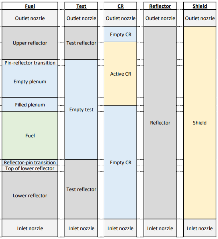
Figure 2: Axial configuration of the VTR fuel assemblies.
Table 1: Driver Fuel Assembly Dimensions, taken from (Shemon, Emily R. et al., 2020).
| Parameter | Cold Dimension | Unit |
|---|---|---|
| Assembly Pitch | 12 | cm |
| Duct flat-to-flat | 11.7 | cm |
| Duct thickness | 0.3 | cm |
| Number of rods | 217 | - |
| P/D | 1.18 | - |
| Cladding outer radius | 0.3125 | cm |
| Cladding thickness | 0.0435 | cm |
| Sodium bond thickness | 0.0360 | cm |
| Fuel slug radius | 0.2330 | cm |
| Wire Wrap | yes | - |
| Active fuel length | 80 | cm |
Table 2: Control Rod Dimensions, taken from (Shemon, Emily R. et al., 2020).
| Parameter | Cold Dimension | Unit |
|---|---|---|
| Assembly Pitch | 12 | cm |
| Inter-assembly gap | 0.3 | cm |
| Outer duct outside flat-to-flat | 11.7 | cm |
| Outer duct inside flat-to-flat | 11.1 | cm |
| Outer duct thickness | 0.3 | cm |
| Inner duct sodium gap thickness | 0.3 | cm |
| Inner duct outside flat-to-flat | 10.5 | cm |
| Inner duct inside flat-to-flat | 9.9 | cm |
| Number of rods | 37 | - |
| P/D. | 1.02231 | - |
| Cladding outer radius | 0.7398 | cm |
| Cladding thickness | 0.0825 | cm |
| Helium bond thickness | 0.0514 | cm |
| B4C absorber radius | 0.6060 | cm |
| Wire wrap | yes | - |
.](../../media/vtr/vtr_fuel_loading.png)
Figure 3: Fuel Management Strategy, taken from (Heidet, F. and Roglans-Ribas, J., 2021).
VTR model description
This VTB model provides a conceptual design to the proposed VTR. Reactor core analyses of the VTR, or more generally SFRs, require the modeling of multiple physics systems, such as:
Neutron flux distribution throughout the core, obtained by solving the neutron transport equation.
Coolant temperature and density distribution, obtained by solving the thermal-hydraulic equation system for the flowing sodium.
Fuel temperature distribution, obtained by solving the heat conduction equation in the fuel rods.
Due to the large temperature gradients occurring in SFR cores, thermal expansion plays a significant role and needs to be accounted for by computational models.
The VTR model captures the predominant feedback mechanisms and consists of 4 independent application inputs:
A 3D Griffin neutronics model, whose main purpose is to compute the 3D neutron flux / power given the local field temperatures and mechanical deformations due to thermal expansion.
A 2D axisymmetric BISON model of the fuel rod which predicts the thermal response given a power density, as well as the thermal expansion occurring in the fuel/clad materials. The predicted quantities (fuel temperature, axial expansion in the fuel) are then passed back to the neutronics model. One BISON input is instantiated per fuel assembly.
A tensor mechanic input of the core support plate, predicting the stress-strain relationships given the inlet sodium temperature. The displacements are passed to the neutronics model to account for the radial displacements in the core geometry. Since the core support plate expansion is tied to the inlet temperature (fixed in this analysis), this model is only called once at the beginning of the simulation.
A SAM 1D channel input, whose purpose is to compute the coolant channel temperature / density profile and pressure drop, given the orifice strategy selected which dictates the input mass flow rate and outlet pressure and the wall temperature coming from the BISON thermal model. The coolant density and heat transfer coefficient is passed back to BISON to be used in a convective heat flux boundary condition. The coolant density is also passed back to the neutronics model for updating the cross sections. One SAM input is instantiated per coolant channel. The coupling scheme with the variables exchanged between solvers is given in Figure 4.
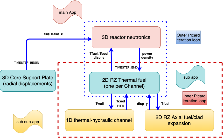
Figure 4: The coupling scheme used for the SFR model.
Griffin Neutronics Model
Griffin Calculation Scheme
The Griffin neutronics computational model relies on the two-step approach:
Cross section spatial homogenization and group condensation using the flux solution from a high-order transport calculation. Typically, for advanced reactors, a 3D continuous-energy Monte Carlo transport calculation is employed to generate the multigroup cross sections and reference fluxes for the second step.
Low-order transport solution, using the multigroup cross sections generated at Step 1, with an optional equivalence step that recaptures the homogenization error as well as the remaining spatial/angular/energy discretization errors. In this model, the Continuous Finite Element Method (CFEM) multigroup diffusion approximation with SPH equivalence is employed (Labouré et al., 2019).
This section details the equations in place in the Griffin neutronics model. The multi-group diffusion equation.
(1)
with the following reflective (Neumann) and vacuum (Robin) boundary conditions, defined respectively by:
In the above equations, is the number of energy groups, is the scalar flux, is the diffusion coefficient, and , and are the macroscopic removal, fission, and scattering cross sections, respectively. is the outward normal unit vector on the boundary .
In general, Eq. (1) does not reproduce the reference reaction rates and multiplication factor . SPH factors are introduced to correct the multigroup cross sections for each reaction (removal, fission, scattering) in each equivalence region, and energy group in such a way that the reaction rates from the reference calculation and from the low-order, diffusion equation are equal:
For each equivalence region and energy group , the reaction rates can be defined as:
The SPH-corrected neutron diffusion equation is then written as:
(2)
These reference fluxes and cross-section sets are generated by Serpent for different combinations of perturbations for the selected cross-section variables (burnup, fuel temperature, etc.), which are also referred to as parameters. The combinations of these parameters define statepoints.
Cross-Section Model
There exists an intermediate step in the two step method that allows for the cross section evaluation at an arbitrary state point. This is typically considered as a cross-section parametrization, which depends on the type of analysis to perform and reactor type. As a general rule, the state variables need to capture the important feedback mechanisms (i.e., the ones that lead to significant changes in cross sections, and thus in reactivity). Then, once these state parameters are identified, it is equally important to cover the full range of variation of each parameter, to avoid extrapolating the cross sections outside of the points used to build the model. The Griffin cross-section model also requires the grid to be full, meaning that the total number of statepoints increases exponentially with the dimensions (or number of points) used per parameter ().
This study's purpose is to perform only steady-state analyses, thus the parameter selection is primarily dictated by the verification of the reactivity coefficients. The selected reactivity coefficients that require careful selection of the cross-section parametrization are the fuel temperature (Doppler), the coolant density/temperature, and the control rod insertion fraction. Other parameters that capture changes in reactivity due to mechanical deformation, such as axial or radial expansion, are covered directly by the mesh deformation capability of Griffin. The cross-section parametrization can be written using a functional formulation:
where is approximated by a piece-wise linear function that uses the local parameter values at each element of the mesh coming from the other physics models.
The grid selected for each parameter is:
.
The maximum fuel temperature was selected to coincide with the value used for generating a Doppler coefficient (1800 K). No changes in density were applied when varying the fuel temperature during the cross-section generation process. It is justified since the BISON model documented in BISON Thermal Model will provide the change in fuel temperature. Changes in the fuel density (e.g., due to thermal expansion) will be accounted for by the mesh deformation capability of Griffin and will be presented later.
The change in coolant temperature is actually capturing the change in coolant density, and the cross sections were generated in Serpent by using the sodium density corresponding to each temperature. The temperatures selected correspond to a 3% change in sodium density, which was arbitrarily selected to cover the perturbation range used for the sodium density coefficient (+1%). Using the sodium density correlation, a 3% change in density corresponds to 103 K. Both parameters could be then used in Griffin (either temperature or density, since density is a bijective function of the temperature), as long as consistent data is passed from the thermal hydraulic model. Note that the Serpent model includes an axial variation in coolant density/temperature, corresponding for the nominal case to 623 K at the bottom inlet and bottom reflector region, 698 K in the active core region, and 773 K in the top region. The temperature axial profile is uniformly increased or decreased by a value corresponding to K for the perturbed cases.
The control rod insertion fraction is selected to preserve the control rod worth. For now, only the primary control rod system is modeled, but it is possible to extend it to model the secondary control rod system as well.
The SPH factors are then computed by Griffin at the selected statepoints and saved in the cross-section library. The resulting data set consisting of multigroup data (cross sections, kinetics parameters, and SPH factors) can be then used in a multiphysics simulation where the local conditions (fuel temperature, etc.) are provided by the thermal physics models.
The energy mesh applied is specifically optimized for generating cross sections for fast spectrum reactors with a Monte Carlo code, and it was originally proposed in Cai (2014) by collapsing the ECCO 33 energy groups into six. The boundaries are provided in Table 3.
Table 3: Energy mesh used for the multigroup cross-section condensation.
| Group | Lower Boundary (MeV) | Upper Boundary (MeV) |
|---|---|---|
| 0 | 2.2313 | 20.0 |
| 1 | 0.49787 | 2.2313 |
| 2 | 4.0868e-2 | 0.49787 |
| 3 | 9.1188e-3 | 4.0868e-2 |
| 4 | 3.354626e-3 | 9.1188e-3 |
| 5 | 1.00e-11 | 3.354626e-3 |
The spatial mesh used in Griffin is generated with CUBIT SNL (2012) and shown in Figure 5 and Figure 6. As for the Serpent VTR model, each driver fuel assembly is split uniformly in five axial layers. Each axial layer has a separate set of cross sections coming from the Serpent calculation. Only beginning of equilibrium cycle (BOEC) results are presented in this study, but this research can be easily extended to include end of equilibrium cycle results or any given burnup value.

Figure 5: Griffin Mesh (radial).
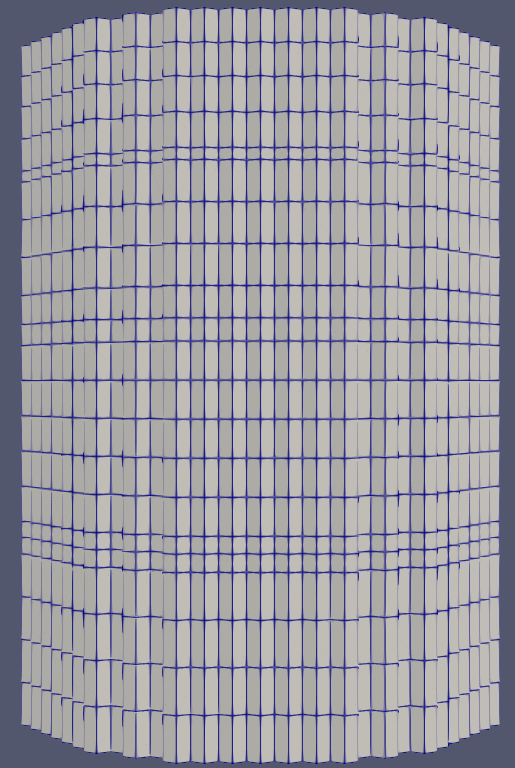
Figure 6: Griffin Mesh (axial).
As mentioned above, the changes in dimensions, due for instance to eigenstrains, are not modeled through a cross-section parametrization, such as a variation in lattice pitch or other change requiring additional 3D Monte Carlo calculations. Rather, the changes occurring in the finite element mesh lead to a change in the associated volumes relative to the non-deformed mesh that is automatically detected by Griffin and used to modify the corresponding cross sections. Using Lagrangian notations, the displacement vector and its associated gradient are related to the strains via strain-displacement relations (more details will be given on the mechanical equations used in BISON Mechanical Model). Once the displacements are obtained, the changes in material densities can be computed via
Each macroscopic cross section is then corrected to account for the changes in the mesh dimension:
where stands for the reaction type (absorption, fission, scattering, removal). This model is fairly unique and has the advantage of significantly simplifying the coupling of Griffin with tensor mechanics problems. It however assumes that the density perturbations do not affect the spectrum significantly and thus that the microscopic cross sections are not changed. This assumption will be verified in VTR Results by comparing the Griffin results against explicit mesh-deformed Serpent calculations.
Description of the BISON Thermo-Mechanical Model
For each fuel assembly, a representative fuel rod is modeled using the BISON code. A 2D axisymmetric representation of the rod geometry is used, as depicted in Figure 7. The purpose of this model is multiple for this analysis. First, it captures changes in fuel temperature due to changes in power density and thus is tightly coupled to the neutronics model, as a change in fuel temperature will change the multigroup cross sections, which will change the power density, and so forth. It also models the axial thermal expansion of the fuel rod resulting from an increase in the fuel temperature. The axial expansion of the fuel is also tightly coupled to the neutronics model, primarily via a geometrical effect (increased fuel rod dimensions, thus increased neutron leakage) and to a lesser extent, with a density effect (less fissile material per volume), which will change the power density, thus the fuel temperature, and therefore the axial expansion itself. These feedback mechanisms are usually ignored in most SFR computational schemes where only a loose coupling strategy is applied. The BISON model also provides the wall (outer clad) temperature profile for use in the coolant channel calculation, which passes back the bulk coolant temperature and heat transfer coefficient that are applied as a Robin boundary condition in BISON. Thus, the thermo-mechanical model is tightly coupled with the thermal-hydraulic model. Second, the BISON model will provide estimates for key safety limits, such as peak centerline temperature and peak cladding temperature. In this study, these quantities are based on average power density levels and do not account for variations in rod-to-rod power level, which can be easily performed as a next step.
Coupling both the heat conduction and the momentum conservation PDEs into a single solve (fully coupled approach) was found to be difficult from a numerical standpoint and often resulted in solve failures. A more robust approach was to dissociate the thermal feedback from the mechanical one. For each fuel assembly, two BISON inputs were created, sharing the exact same geometry but upon which different physics are solved:
One input solving only the heat conduction problem across the fuel rod
One input modeling the mechanical expansion in the fuel and clad as a function of the temperature.
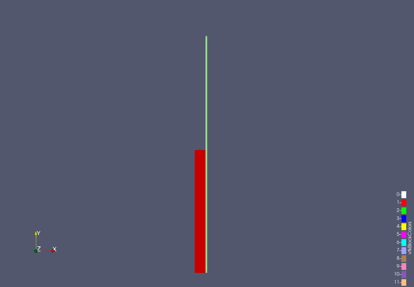
Figure 7: BISON 2D RZ geometry with aspect ratio modified.
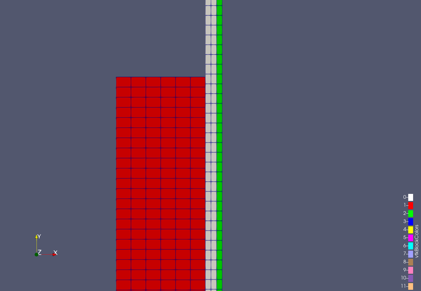
Figure 8: BISON spatial mesh.
BISON Thermal Model
The steady-state heat conduction equation solved is:
(3)
with the following Neumann boundary condition for :
and a Robin boundary condition on the outside clad surface of radius :
with as the convective heat transfer coefficient and as the bulk coolant temperature, which are computed by SAM (see Description of the SAM Thermal-Hydraulic Model for the correlations used). The power density for the fuel rod corresponds to the average power density per rod for each assembly. It is obtained by normalizing the power density computed by Griffin on the homogenized fuel assembly so as to preserve the power between both volumes:
where:
: number of rods per assembly
: power density in calculated in Griffin for the 3D homogeneous fuel assembly, whose corresponding volume is
: power density in to be used in BISON for the 2D RZ heterogeneous fuel pin, whose corresponding volume is
: slug outer radius ()
: slug length ().
In practice, the power density in BISON is the power density from Griffin scaled up by a normalization factor :
Currently, the model assumes that all the fission power is locally deposited in the fuel rod. The material properties utilized by this model are the thermal conductivity and the heat capacity for the metallic fuel and the HT9 cladding. BISON incorporates these properties internally, and for the ternary UPuZr metallic fuel, different correlations are available. For this study, the fresh fuel thermal conductivity from Billone (1986) is used, with the Savage model for the fuel heat capacity Savage (1968). The cladding material properties are based on Hofman et al. (1997).
BISON Mechanical Model
The BISON mechanical model solves the steady-state form of the conservation of momentum for solid mechanics on the same 2D axisymmetric mesh as the thermal model:
Where is the nominal stress tensor, is the displacement, and with the following boundary conditions:
We rely on the infinitesimal strain theory, which linearly relates the stress and displacement tensors. The displacement is assumed to be much smaller than any relevant dimensions so that its geometry and the constitutive properties of the material (such as density and stiffness) at each point of space can be assumed to be unchanged by the deformation. The nominal stress tensor is directly related to the symmetric strain tensor and the thermal expansion for isotropic materials:
where and are Lame constants, which depend on Young's modulus and Poisson's ratio :
is the thermal expansion coefficient, the strain-free temperature, represents a trace operation on a tensor, and is the identity tensor. The strain tensor is evaluated from the displacement with the strain-displacement equations:
The temperature is an input, transferred from the BISON thermal model.
The mechanical properties used in this model consist of the Young's modulus and Poisson's ratio that are required to build the elasticity tensor, as well as the thermal expansion eigenstrains. As for the thermal material properties, BISON incorporates these models internally. Correlations used for Young's modulus and Poisson's ratio for the ternary metallic fuel are based on Hofman et al. (1997), while the thermal expansion eigenstrain is taken from Geelhood and Porter (2018). The HT9 cladding Young's modulus and Poisson's ratio are based on correlations from Maloy et al. (2008). The HT9 thermal expansion coefficient is provided in Leibowitz and Blomquist (1988).
Description of the SAM Thermal-Hydraulic Model
A single channel model is used for this analysis, for which the inlet temperature and outlet pressure are imposed as boundary conditions. The mass flow rate and sodium velocity are dependent upon the orifice type. Currently, orifices are only defined for the active core region, as shown in Figure 9. SAM relies on a 1D single-phase flow model. The governing equations are documented in Section 2.1 of the SAM theory manual Hu et al. (2021). The wall surface temperature , provided by the BISON calculation, is used in the conjugate heat transfer model at the clad surface. The convective heat flux is then:
where and are the heat transfer coefficient and the bulk coolant temperature, respectively.
There are two closure models required, one for the determination of the (forced) convective heat transfer coefficient and one for the wall friction. By default, SAM uses the Calamai/Kazimi-Carelli correlation for estimating the convective heat transfer coefficient for bundle geometries with sodium as a fluid, see Section 5.1.2.2 of Hu et al. (2021) for a complete description. For the wall friction, the simplified version of Cheng-Todreas correlation is applied for wire-wrapped rod bundles (see Section 5.2.2 of Hu et al. (2021).
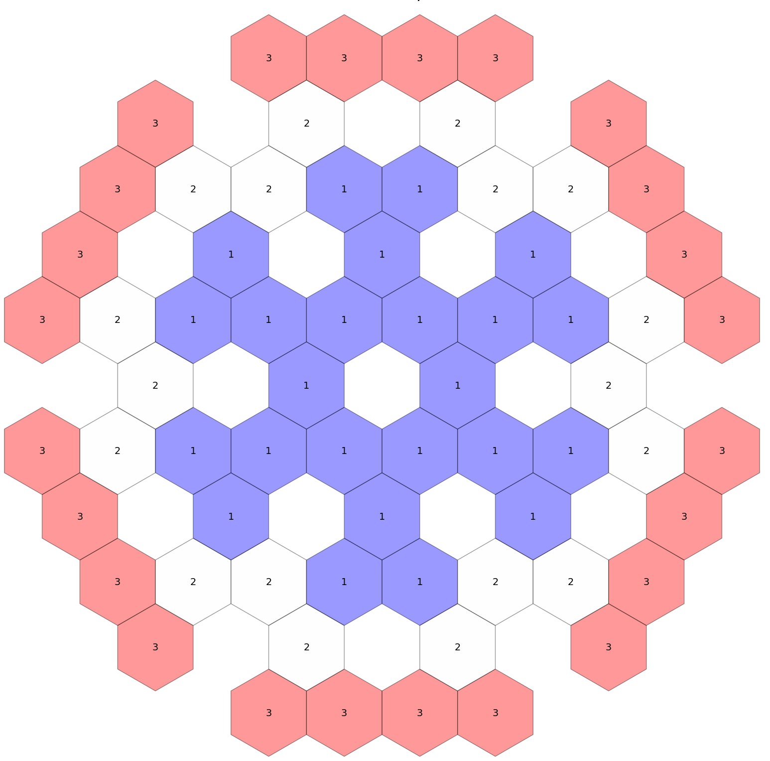
Figure 9: Orifice map
Description of the Core Support Plate Model
A 3D model of the core support plate is built using the MOOSE tensor mechanics module. The equations given in BISON Mechanical Model apply to this model as well. The mesh used for the core support plate is given in Figure 10 and Figure 11. The core support plate is assumed to be fixed at its center (0,0,0), as well at the bottom plane (y=0), and expand freely in the radial directions, as well as in the upward direction. Only the radial displacements are connected to the neutronics model in the multiphysics scheme, so the thermal expansion of the core support plates leads to an increase in fuel assembly pitch, but not a shift in core height.
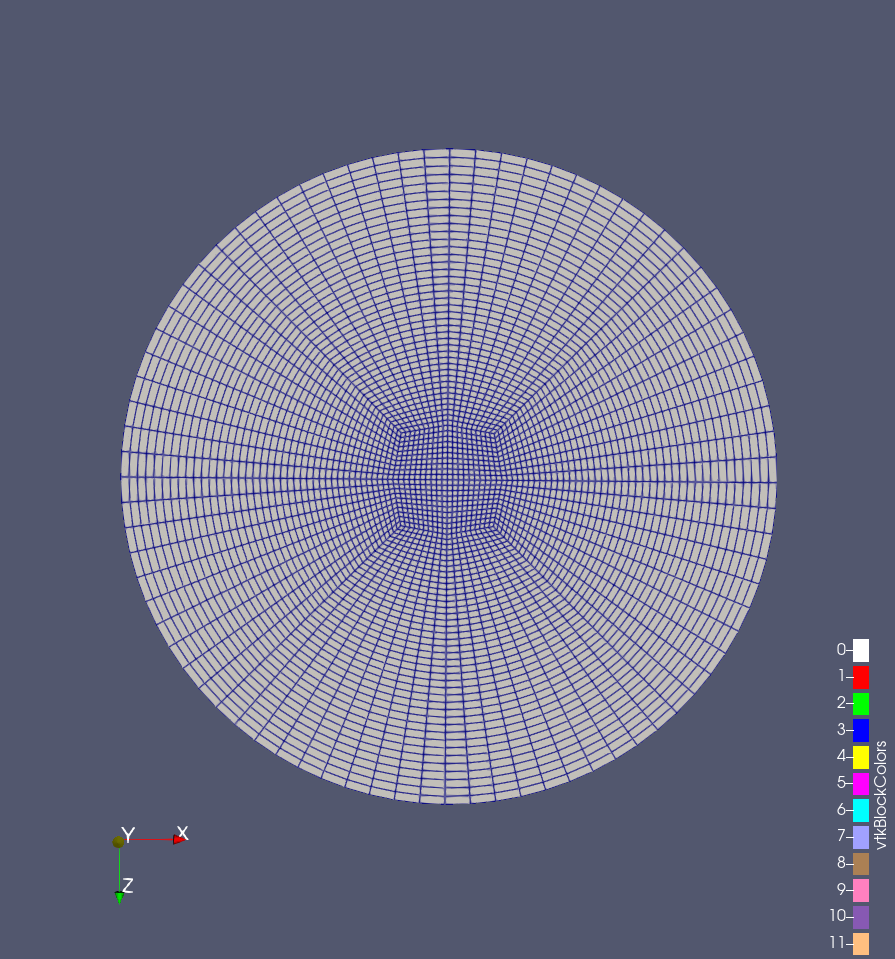
Figure 10: Core support plate radial mesh.
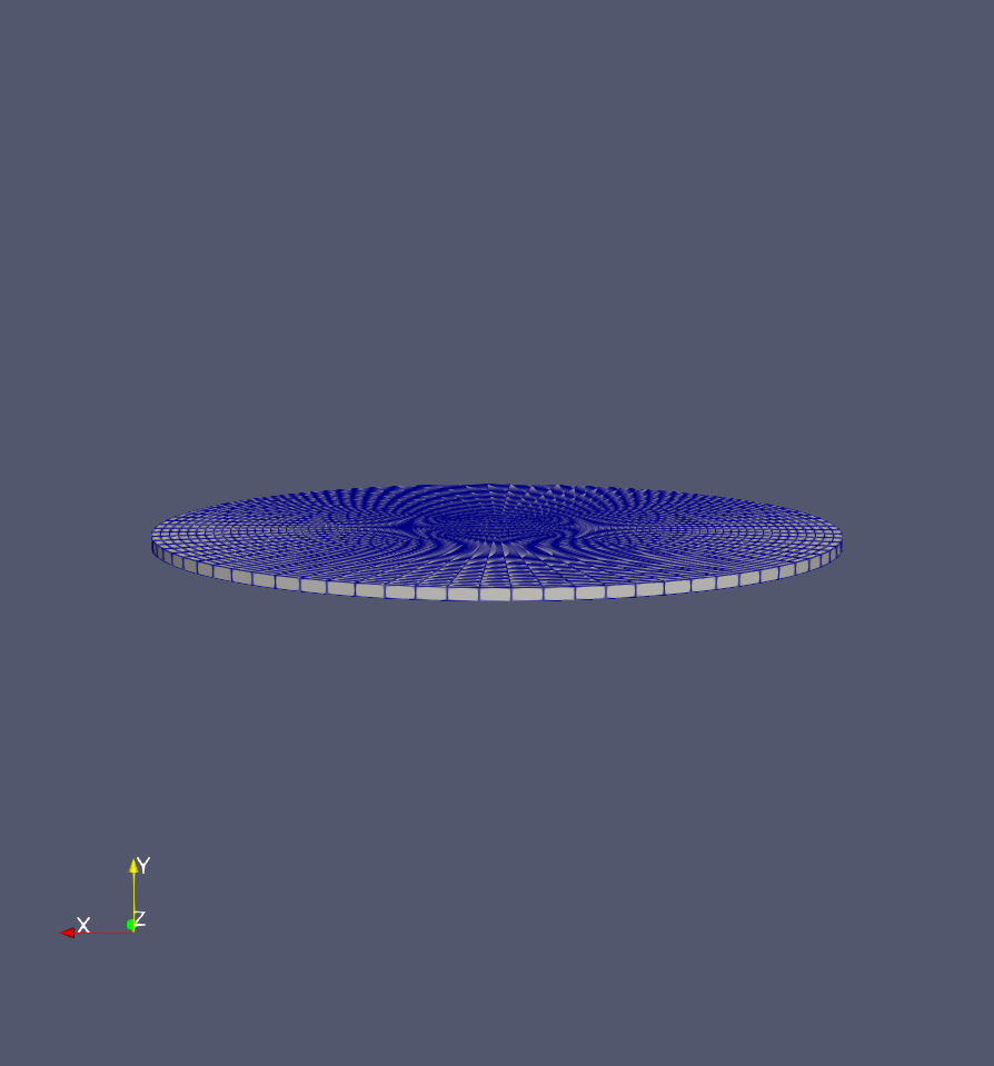
Figure 11: Core support plate axial mesh.
The BISON internal mechanical properties for stainless steel 316 are used. The Poisson's ratio is held constant (). The Young's modulus in Pa is computed using:
The thermal expansion coefficient is based on data extracted from ASME (2016).
How to run the model
The neutronics-only model can be ran with Griffin.
Run it via:
griffin-opt -i griffin_only.i
The multi-physics model relies on the BlueCrab app, which incorporates the different required applications (Griffin, BISON, SAM).
Run it via:
mpirun -n 48 blue_crab-opt -i griffin_multiphysics.i
Acknowledgments
This model is adapted from (Martin, Nicholas et al., 2022) and prepared for the VTB by Thomas Folk.
References
- ASME.
ASME Boiler and Pressure Vessel Code, chapter II, Part D. 16Cr-12Ni-2Mo (Group 3).
The American Society of Mechanical Engineers, New York, N.Y., 2016.[BibTeX]
- M. C. Billone.
Status of fuel element modeling code for metallic fuels.
Int. Conf. Reliable Fuels for Liquid Metal Reactors, Tucson, Arizona, Sep. 7-11, 1986, 1986.
URL: https://ci.nii.ac.jp/naid/10026451881/en/.[BibTeX]
- Li Cai.
Condensation and homogenization of cross sections for the deterministic transport codes with Monte Carlo method : Application to the GEN IV fast neutron reactors.
PhD thesis, Université Paris-Sud, 2014.[BibTeX]
- KJ Geelhood and IE Porter.
Modeling and assessment of ebr-ii fuel with the us nrcs fast fuel performance code.
2018.[BibTeX]
- G.L. Hofman, L.C. Walters, and T.H. Bauer.
Metallic fast reactor fuels.
Progress in Nuclear Energy, 31(1):83–110, 1997.
The Technology of the Integral Fast Reactor and its Associated Fuel Cycle.
URL: https://www.sciencedirect.com/science/article/pii/0149197096000054, doi:https://doi.org/10.1016/0149-1970(96)00005-4.[BibTeX]
- Rui Hu, Ling Zou, Daniel Nunez, Travis Mui, and Tingzhou Fei.
SAM Theory Manual.
Argonne National Laboratory, 2021.[BibTeX]
- Vincent Labouré, Yaqi Wang, Javier Ortensi, Sebastian Schunert, Frederick Gleicher, Mark DeHart, and Richard Martineau.
Hybrid Super Homogenization and Discontinuity Factor Method for Continuous Finite Element Diffusion.
Annals of Nuclear Energy, 128(INL/JOU-18-5106):443–454, June 2019.
doi:10.1016/j.anucene.2019.01.003.[BibTeX]
- L. Leibowitz and R.A. Blomquist.
Thermal conductivity and thermal expansion of stainless steels d9 and ht9.
International Journal of Thermophysics, 9(5):873–883, 1988.
cited By 55.
URL: https://www.scopus.com/inward/record.uri?eid=2-s2.0-1642313943&doi=10.1007%2fBF00503252&partnerID=40&md5=8464d5679b097d19934fcb31b427119f, doi:10.1007/BF00503252.[BibTeX]
- Stuart Maloy, Berylene Rogers, Weiju Ren, and Philip Rittenhouse.
Status of materials handbooks for particle accelerator and nuclear reactor applications.
Journal of Nuclear Materials, 377(1):94–96, 2008.
Spallation Materials Technology.
URL: https://www.sciencedirect.com/science/article/pii/S0022311508001207, doi:https://doi.org/10.1016/j.jnucmat.2008.02.056.[BibTeX]
- A. G. Nelson, D.C. Crawford, and F. Heidet.
Versatile test reactor: core system design requirements to support advanced reactor development.
Int. Conf. on Fast Reactors and Related Fuel Cycles, Beijing, China, Apr. 25-28, 2022, 2022.[BibTeX]
- H. Savage.
The heat content and specific heat of some metallic fast-reactor fuels containing plutonium.
Journal of Nuclear Materials, 25(3):249–259, 1968.
URL: https://www.sciencedirect.com/science/article/pii/0022311568901682, doi:https://doi.org/10.1016/0022-3115(68)90168-2.[BibTeX]
- SNL.
CUBIT 13.2 User Documentation.
2012.
URL: https://tinyurl.com/rgsbqb7.[BibTeX]
- Heidet, F.
Versatile test reactor: conceptual core design overview.
Int. Conf. on Fast Reactors and Related Fuel Cycles, Beijing, China, Apr. 25-28, 2022, 2022.[BibTeX]
- Heidet, F. and Roglans-Ribas, J.
Core design activities of the versatile test reactor - conceptual phase.
EPJ Web Conf., 247:01010, 2021.
URL: https://doi.org/10.1051/epjconf/202124701010, doi:10.1051/epjconf/202124701010.[BibTeX]
- Martin, Nicholas, Stewart, Ryan, and Bays, Sam.
A multiphysics model of the versatile test reactorbased on the moose framework.
Annals of Nuclear Energy, 2022.
URL: https://doi.org/10.1016/j.anucene.2022.109066.[BibTeX]
- Shemon, Emily R., Yu, Yiqi, and Kim, Taek K.
Demonstration of neams multiphysics tools for fast reactor applications.
Technical Report, Argonne National Laboratory, 2020.
URL: https://www.osti.gov/biblio/1671787, doi:10.2172/1671787.[BibTeX]