VTR Results
Griffin Standalone
It is important to verify that the neutronics model reproduces the 3D reference calculations (i.e., that there is no significant discretization and/or homogenization error remaining in the solution). Table 1 provides the comparison of the eigenvalues obtained with Griffin with, and without, SPH equivalence against Serpent. First, it is clear that the Griffin results with SPH equivalence fully reproduce the Serpent ones. Second, as the SPH equivalence recaptures the homogenization error, which is small for fast spectrum reactors, we observe modest differences (around 250 pcm) without SPH equivalence. This relatively low error is due to error compensation effects, as the diffusion approximation should lead to larger discrepancies for a heterogeneous core such as this one. One reason is the usage of the out-scatter approximation for computing the diffusion coefficients in Serpent, which can lead to a too strong transport correction for fast spectrum reactors. For the cases where the control rods are inserted, the Griffin without SPH equivalence are lower compared to Serpent. This is a result of using a homogeneous model where all the B4C-bearing pins are homogenized into one cross-section material, which doesn't capture the neutron flux self-shielding effects. Thus, preserving the rod worth requires the application of an equivalence procedure with the Griffin multigroup diffusion scheme. However, since the bias is almost constant across uncontrolled statepoints, this low error on the could potentially be leveraged for sensitivity analyses without requiring an SPH equivalence as long as the calculations do not involve rodded conditions.
Table 1: differences for the cross-section generation statepoints, with and without SPH equivalence.
| Fuel Temp. (K) | Coolant Temp. (K) | Control Rod Fraction (-) | Serpent | Griffin without SPH | Diff. (pcm) | Griffin with SPH | Diff. (pcm) |
|---|---|---|---|---|---|---|---|
| 600 | 595 | 0.00 | 1.02585 | 1.02848 | 263 | 1.02585 | 0 |
| 600 | 595 | 1.00 | 0.96340 | 0.95802 | -538 | 0.96339 | 0 |
| 600 | 698 | 0.00 | 1.02492 | 1.02747 | 255 | 1.02492 | 0 |
| 600 | 698 | 1.00 | 0.96265 | 0.95719 | -546 | 0.96265 | 0 |
| 600 | 801 | 0.00 | 1.02395 | 1.02644 | 249 | 1.02395 | 0 |
| 600 | 801 | 1.00 | 0.96191 | 0.95634 | -557 | 0.96191 | 0 |
| 900 | 595 | 0.00 | 1.02448 | 1.02699 | 251 | 1.02448 | 0 |
| 900 | 595 | 1.00 | 0.96240 | 0.95695 | -544 | 0.96240 | 0 |
| 900 | 698 | 0.00 | 1.02362 | 1.02600 | 238 | 1.02362 | 0 |
| 900 | 698 | 1.00 | 0.96164 | 0.95610 | -555 | 0.96164 | 0 |
| 900 | 801 | 0.00 | 1.02270 | 1.02500 | 230 | 1.02270 | 0 |
| 900 | 801 | 1.00 | 0.96099 | 0.95527 | -572 | 0.96099 | 0 |
| 1800 | 595 | 0.00 | 1.02229 | 1.02452 | 223 | 1.02229 | 0 |
| 1800 | 595 | 1.00 | 0.96077 | 0.95516 | -561 | 0.96077 | 0 |
| 1800 | 698 | 0.00 | 1.02144 | 1.02358 | 214 | 1.02144 | 0 |
| 1800 | 698 | 1.00 | 0.96007 | 0.95438 | -570 | 0.96007 | 0 |
| 1800 | 801 | 0.00 | 1.02052 | 1.02265 | 213 | 1.02052 | 0 |
| 1800 | 801 | 1.00 | 0.95938 | 0.95354 | -584 | 0.95938 | 0 |
One of the characteristics of the VTR core is the fairly significant number of non-fueled assemblies (reflector and shield assemblies), with two local interfaces, fuel-to-reflector and reflector-to-shield, which present a modeling challenge for deterministic codes such as Griffin. The reflector region is dominated by scattering whereas the fuel and shield regions are dominated by fission and absorption reactions, respectively. As a result, the flux drops significantly in the first few rows of the reflector region and essentially becomes zero in the shield. For instance, Figure 1 provides the fast flux at the core mid-plane.
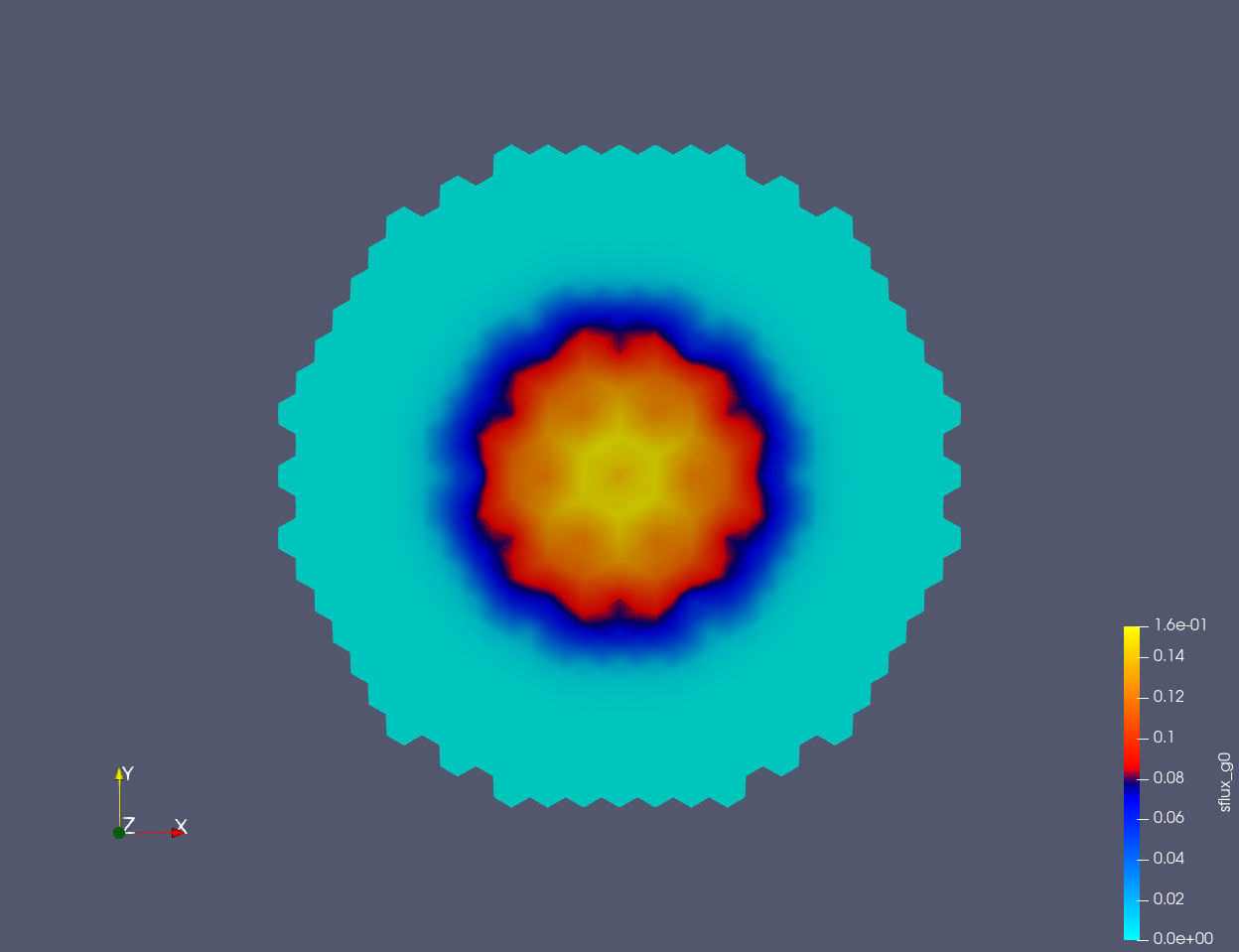
Figure 1: Normalized fast flux at core mid-plane.
Second, a large number of neutrons are reflected back from the reflector region, creating a thermal shift at the core-reflector interface, as can be seen in Figure 2.
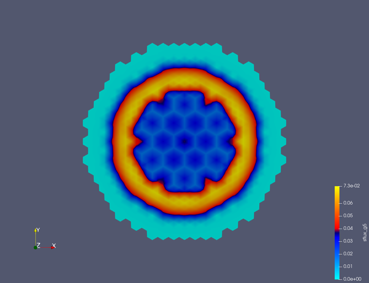
Figure 2: Normalized thermal flux at core mid-plane.
Figure 3 and Figure 4 provide the relative differences between Griffin and Serpent. Without an SPH equivalence, it can be observed that the radial tilt of the flux is poorly predicted (i.e., the flux is overestimated at the core center and becomes underestimated at the reflector region).
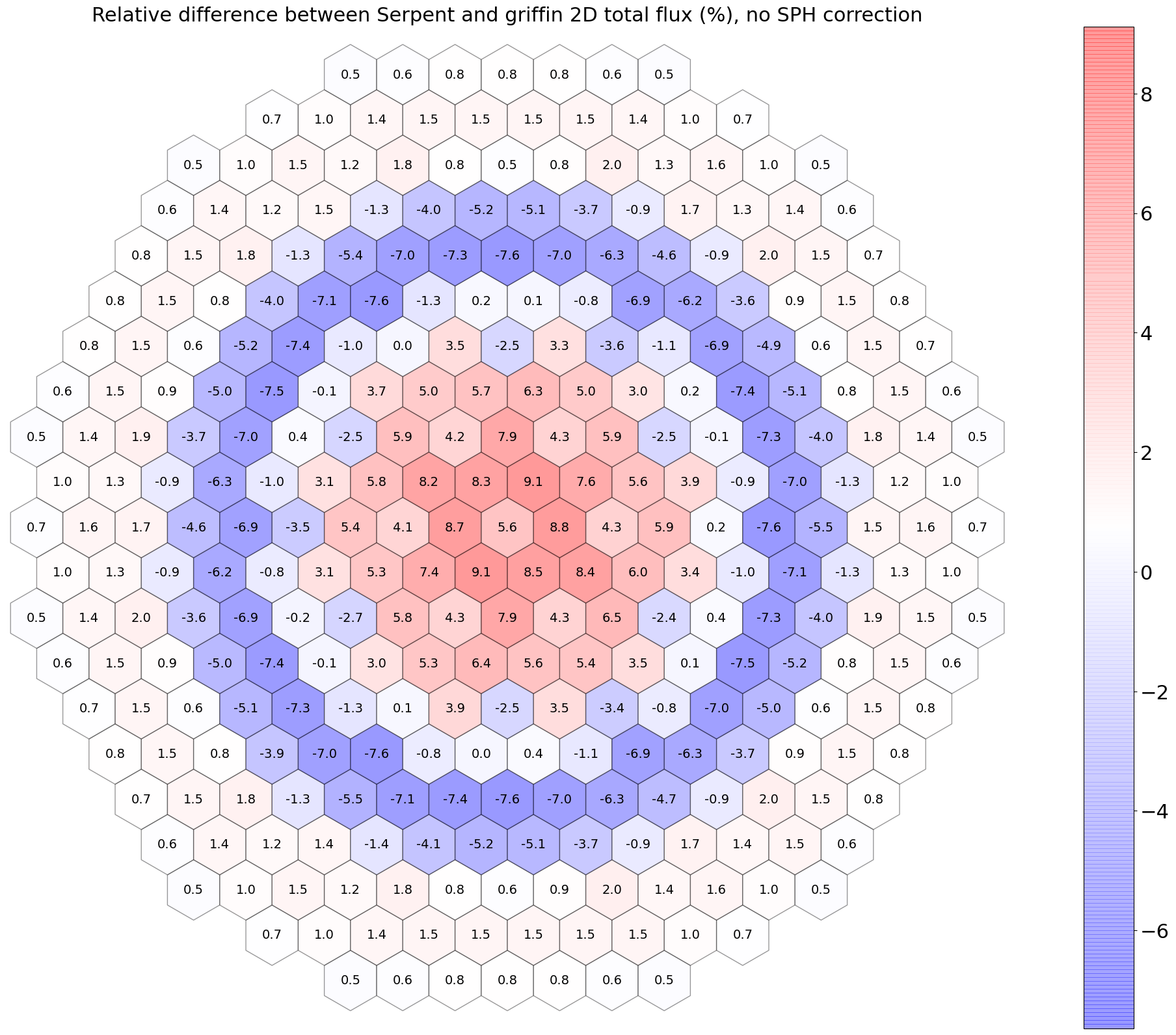
Figure 3: Relative differences in 2D total flux between Griffin and Serpent, no SPH equivalence.
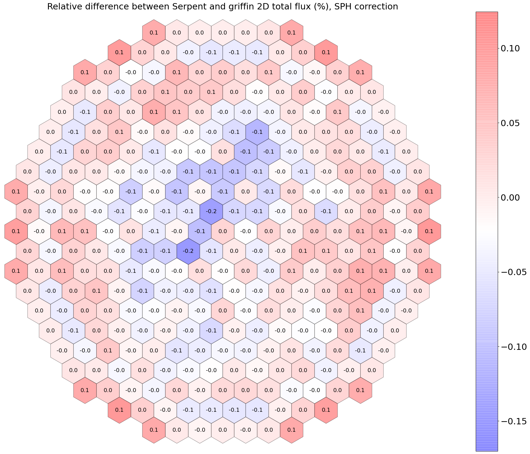
Figure 4: Relative differences in 2D total flux between Griffin and Serpent, with SPH equivalence.
The flux root mean square error (RMSE) is broken down per energy group in Table 2.
Table 2: RMSE for the multigroup flux between Griffin and Serpent (%).
| - | No SPH Equivalence | - | With SPH Equivalence | - |
|---|---|---|---|---|
| Energy Group | RMSE for 2D Flux | RMSE for 3D Flux | RMSE for 2D Flux | RMSE for 3D Flux |
| 0 | 14.38 | 32.30 | 0.57 | 1.58 |
| 1 | 5.67 | 13.97 | 0.14 | 0.34 |
| 2 | 3.56 | 8.39 | 0.05 | 0.15 |
| 3 | 4.31 | 10.32 | 0.12 | 0.35 |
| 4 | 5.73 | 14.86 | 0.39 | 1.49 |
| 5 | 5.01 | 15.41 | 0.23 | 0.86 |
| Total flux () | 3.78 | 8.89 | 0.05 | 0.18 |
Figure 5 and Figure 6 provide the relative differences in 2D fission powers between Griffin and Serpent for the nominal statepoint ( K, K, and CRs out). As expected, the calculations relying on SPH factors preserve the Serpent assembly powers.
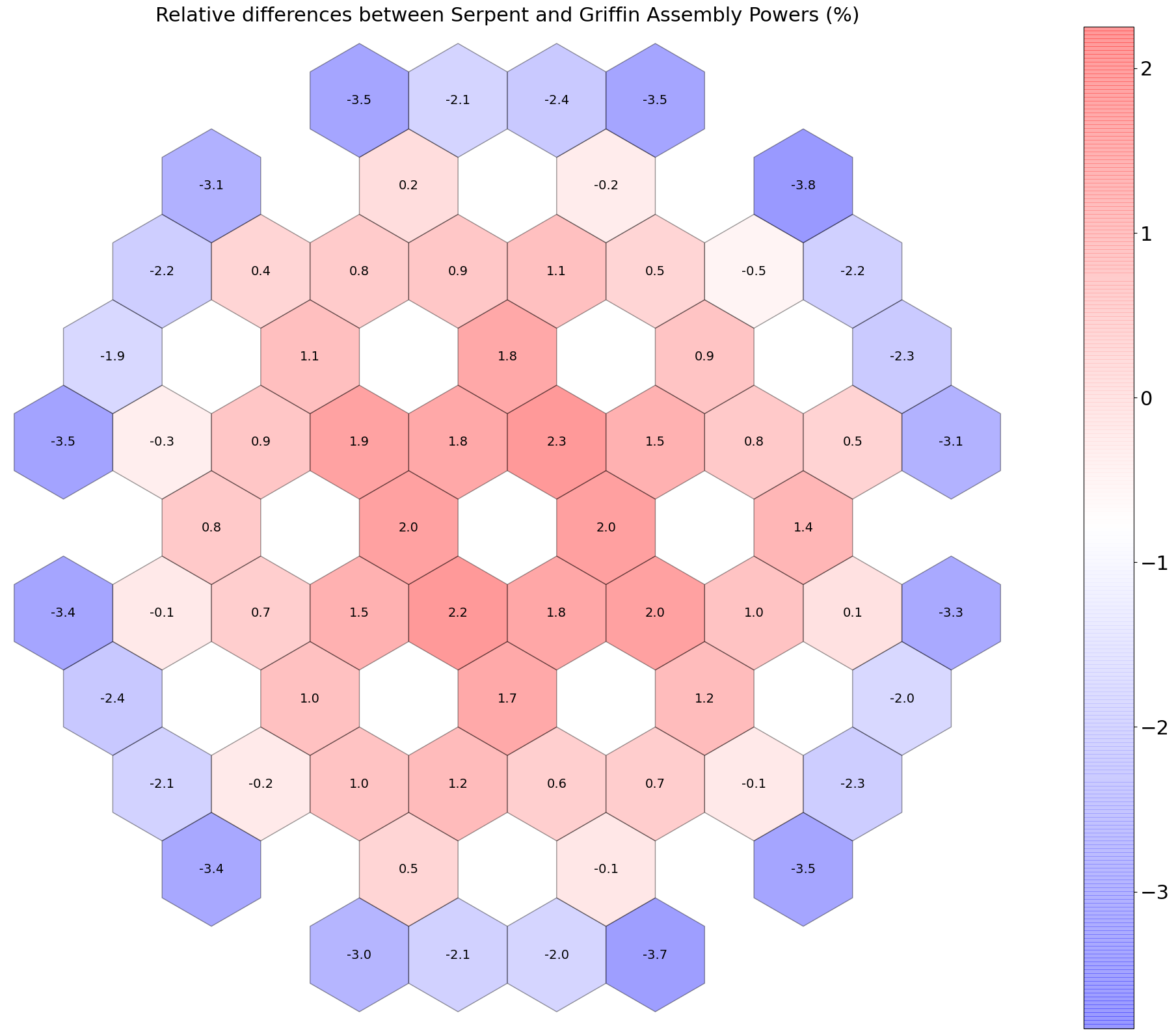
Figure 5: Relative differences in 2D fission power between Griffin and Serpent, no SPH equivalence.
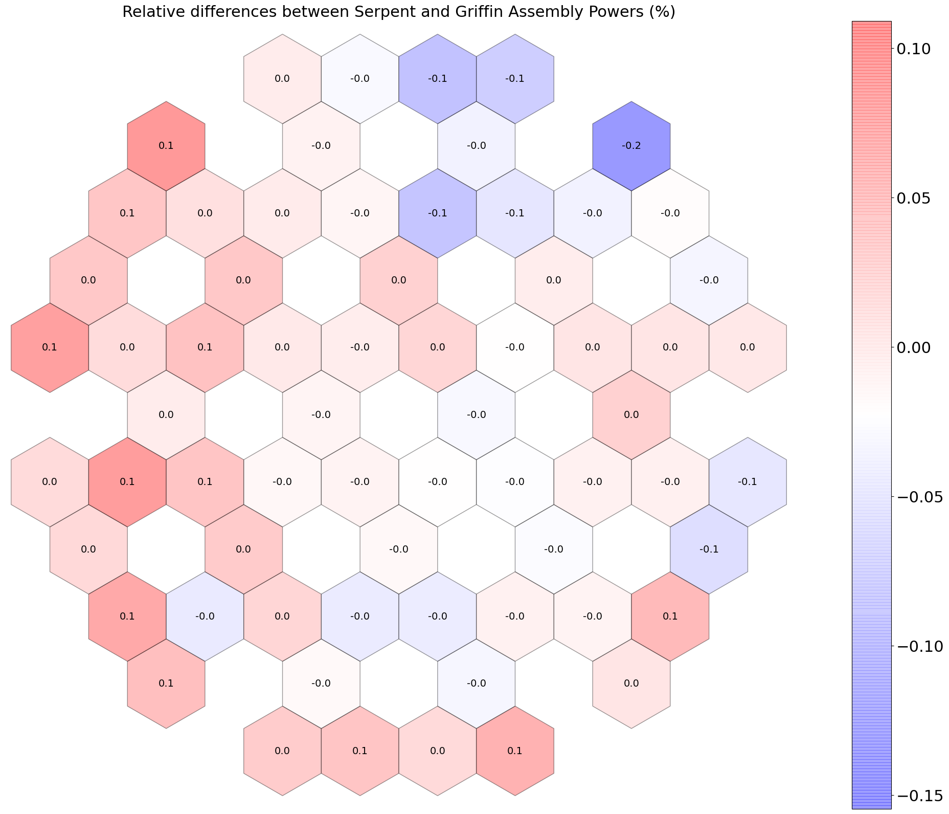
Figure 6: Relative differences in 2D fission power between Griffin and Serpent, with SPH equivalence.
The total rod worth for the six primary rods are computed with Serpent and Griffin. An SPH correction corresponding to the fully inserted and fully withdrawn conditions is required in order to preserve the integral rod worth.
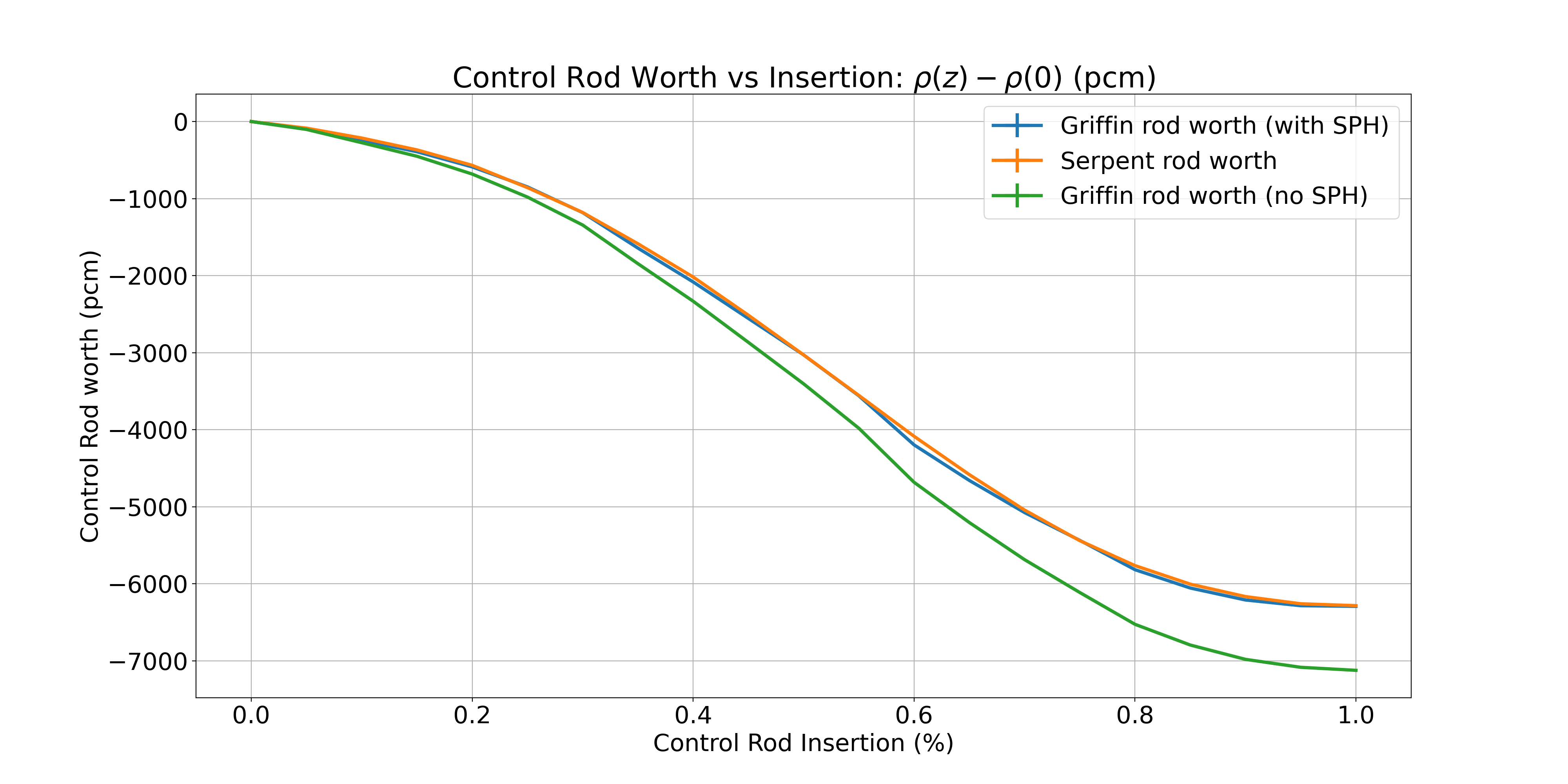
Figure 7: Serpent and Griffin (with and without SPH) control rod worth.
Multi-physics
The results of the multiphysics simulation provide access to the following quantities:
Peak centerline temperatures: Figure 8.
Peak cladding temperatures, on the inner side of the cladding: Figure 9.
Peak bulk coolant temperatures: Figure 10.
Pressure drop per flow channel: Figure 11.
The rod quantities provided are representative of assembly-average power level and do not account for variations in rod-to-rod power and sub-channel flow temperatures. Two features are currently missing in this area within the MOOSE suite of codes employed in this work, namely a sub-channel code, and an efficient transport solver within Griffin for performing heterogeneous pin-by-pin calculations, or alternatively, a pin power reconstruction method that can be employed with coarse-mesh diffusion. Once these capabilities are available, it will be feasible to obtain quantities such as sub-channel and rod-to-rod temperature profiles. A summary of the thermal-hydraulic characteristics corresponding to the three orifice zoning is provided in Table 3.
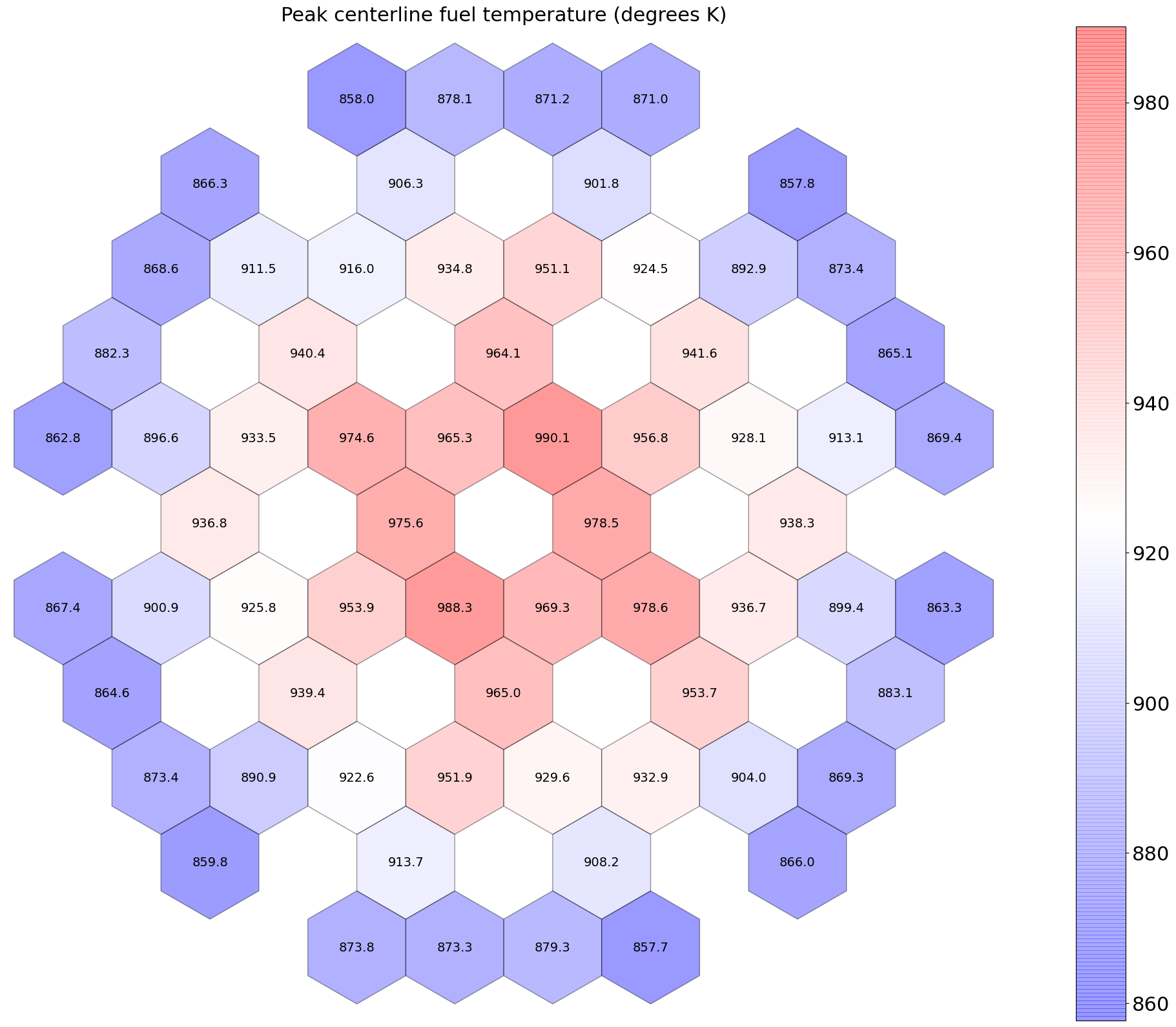
Figure 8: Peak centerline temperatures at BOEC (degrees K).
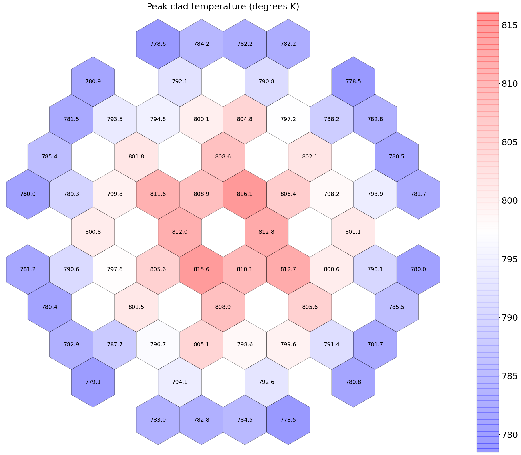
Figure 9: Peak cladding temperatures at BOEC (degrees K).
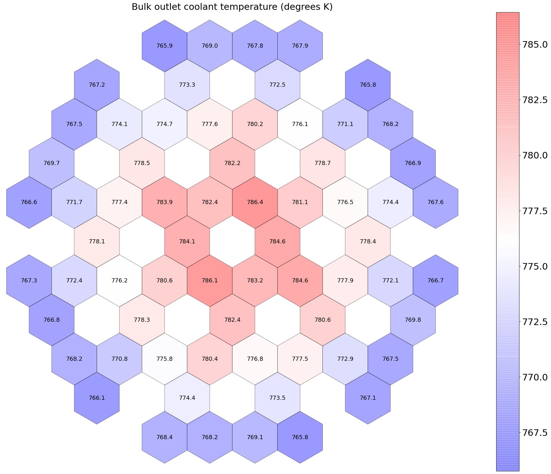
Figure 10: Peak bulk coolant temperatures at BOEC (degrees K).
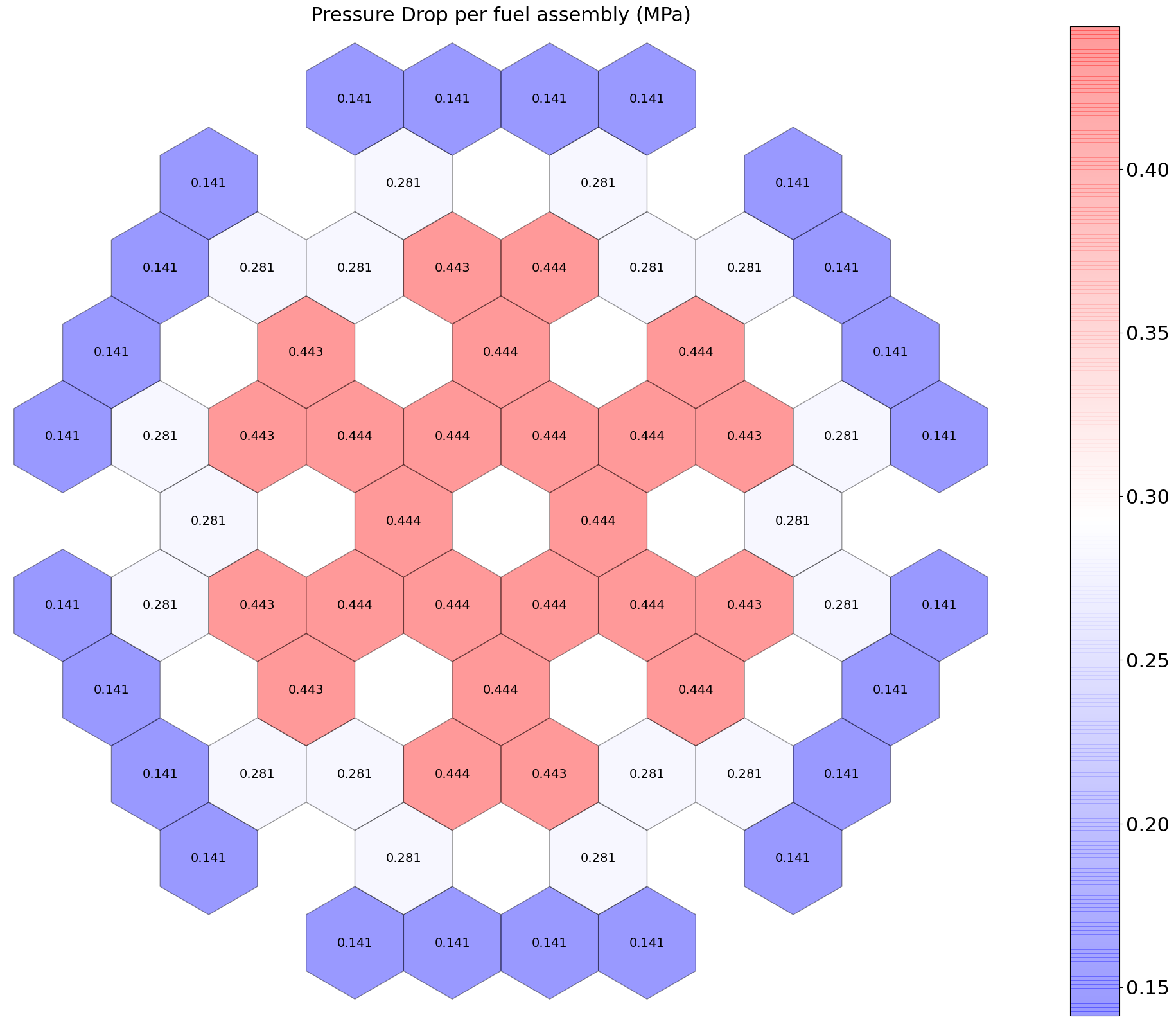
Figure 11: Pressure drop per flow channel.
Table 3: Summary of the thermal-hydraulics characteristics with three orifice groups.
| Orifice Group | - | Flow (kg/s) | Power (MW) | Coolant Bulk Temp. ( K) | Peak Clad Temp. ( K) | Peak Fuel Centerline Temp. ( K) | Pressure Drop (MPa) | Velocity (m/s) |
|---|---|---|---|---|---|---|---|---|
| 1 | avg. max. | 29.8 | 5.81 6.81 | 781 786 | 806 816 | 955 990 | 0.44 | 9.37 |
| 2 | avg. max. | 23.2 | 4.54 5.30 | 774 778 | 794 801 | 912 938 | 0.29 | 7.29 |
| 3 | avg. max. | 15.9 | 3.30 3.68 | 768 770 | 782 786 | 869 883 | 0.15 | 5.00 |
Application of the MOOSE-Based VTR Multiphysics Model
Impact of the Multiphysics Coupling on and Power Distributions
One of the purposes of the MOOSE-based VTR core model is to evaluate the impact of a tight coupling on the neutronics characteristics for steady-state conditions in an SFR core. Two calculations are performed, one using fixed temperature profiles in a standalone neutronics model, and one using the multiphysics model.
The first case assumes a realistic temperature profile in the Serpent input by using an axial variation in coolant density/temperature, corresponding to the nominal case of 623 K at the bottom inlet and bottom reflector region, 698 K in the active core region, and 773 K in the top region, and a uniform fuel temperature of 900 K. These temperatures are representative of what an analyst might pick without access to a detailed thermal-hydraulic solution. The results will depend on the initially chosen temperature profiles, so a better guess might improve the agreement with a coupled multiphysics simulation. The cross sections are fixed during the simulation, since there are no updates in the temperature fields. These cross sections are then employed in Griffin to generate the standalone reference solution.
In the latter case, the neutronics model is tightly coupled to the thermal-hydraulics and thermo-mechanics models, and the cross sections are then updated according to the parametrization described in Cross Section Parameterization. Using a relative convergence criterion of , the calculation converges quickly in five fixed point iterations. The overall CPU time for the multiphysics-coupled calculation on 48 CPU cores (Intel Xeon Platinum 8268, 2.90 GHz) is around 130 seconds.
The with a fixed temperature profile is 1.0236, while with the multiphysics coupling, the is 1.01819, a difference of 543 pcm. The 2D assembly powers, however, are very similar, with maximum relative differences of 1%, as shown in Figure 12. Note that the core assembly powers are not symmetric due to a non-symmetrical fuel loading pattern which is almost, but not quite 1/6-th symmetrical.
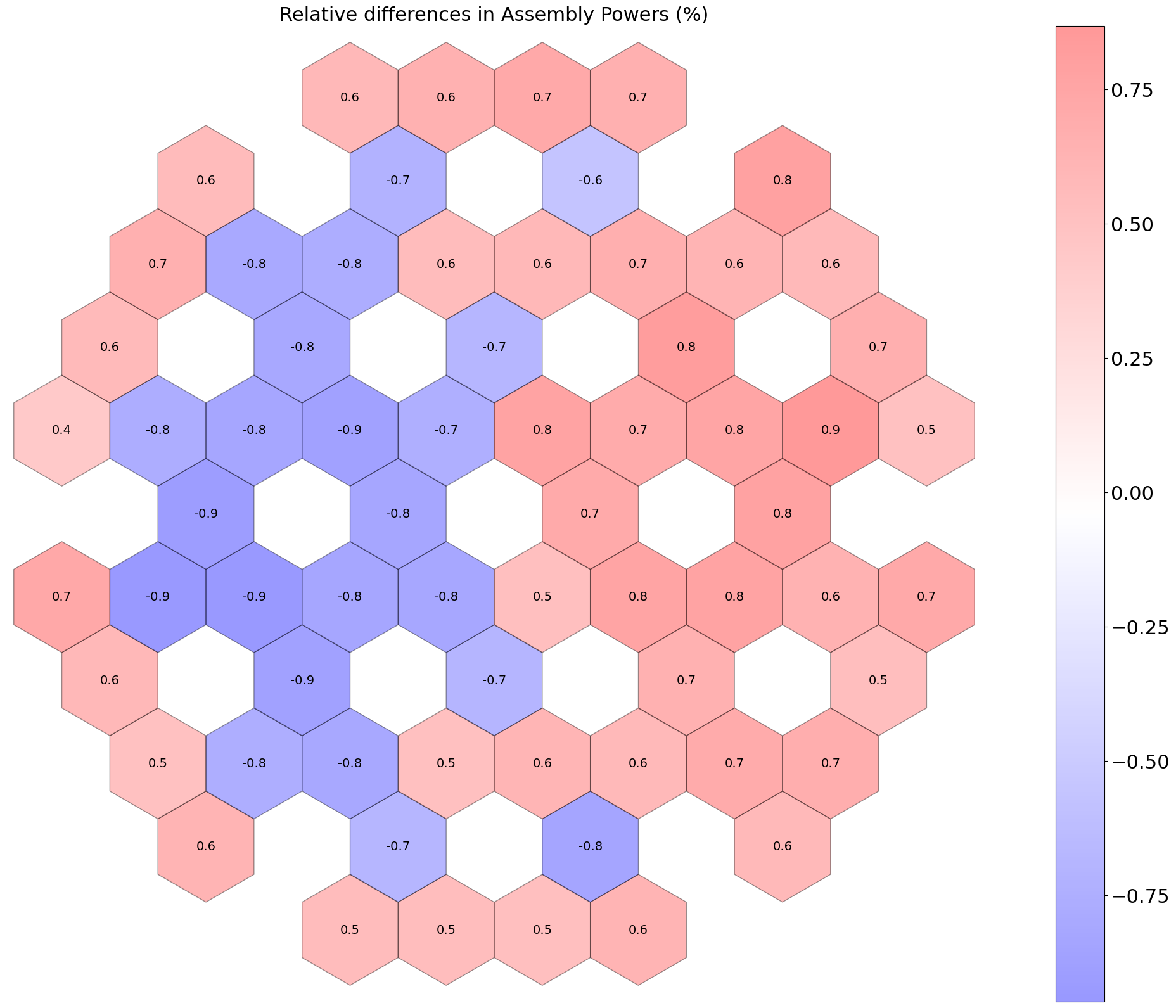
Figure 12: Relative differences in 2D assembly powers, with and without coupling (%).
Figure 13 and Figure 14 provide the axial power for two different assemblies, one located within the first and the second within the third ring of the core, respectively. The maximum relative differences are around -1.4% for the first case, and +1% for the second case.
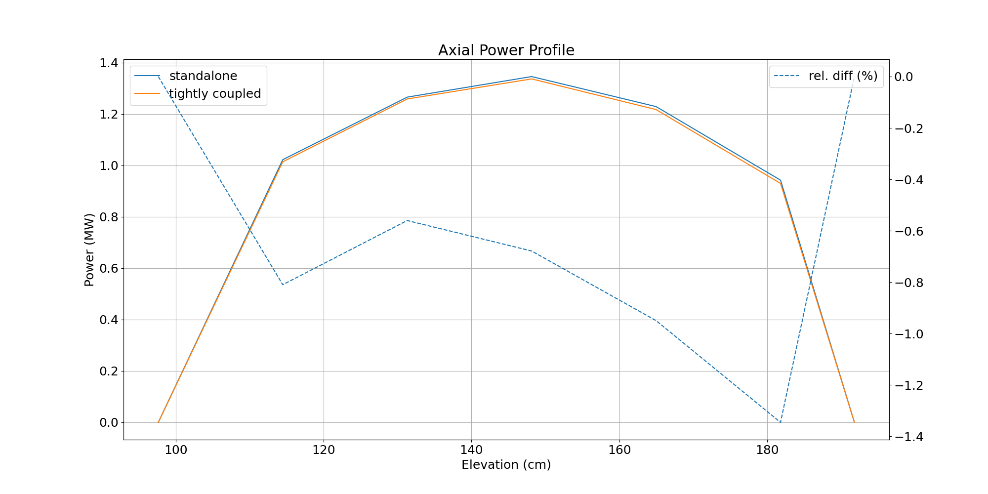
Figure 13: Axial assembly power with and without coupling (first ring).
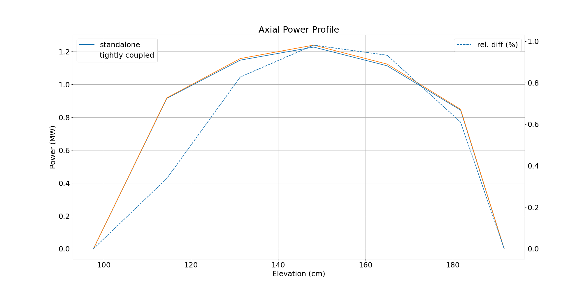
Figure 14: Axial assembly power with and without coupling (third ring).
However the core-average power profile is very similar with and without tight coupling, as can be seen in Figure 15. The axial power profiles for individual assemblies are slightly more impacted, since the differences are induced by axial variations in the temperature fields.
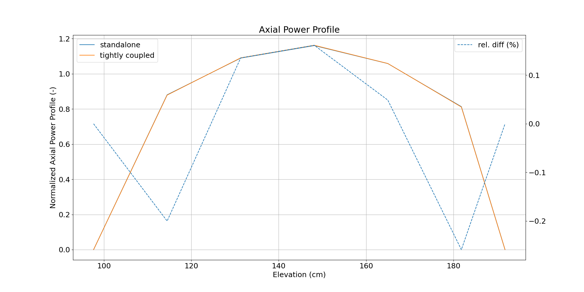
Figure 15: Core-Averaged Axial Power Profile.
Another simulation is performed using a one-way coupling only between the neutronics and the thermal-hydraulics model. There are no iterations between the neutronics and thermal-hydraulics model. Once the neutronics calculation is converged, the power density is passed to the thermal-hydraulics model. The results are then compared to those obtained with the tight-coupling scheme. The differences in peak coolant, clad, and fuel temperatures are negligible, as observed for the peak fuel temperature displayed in Figure 16. Differences for the coolant and clad temperatures are similar and thus not repeated. This result showcases that there are no need to perform fixed point iterations between the neutronics and thermal-hydraulics model for these safety parameters, as a one-way coupling scheme provides almost identical results as the tight-coupling scheme.
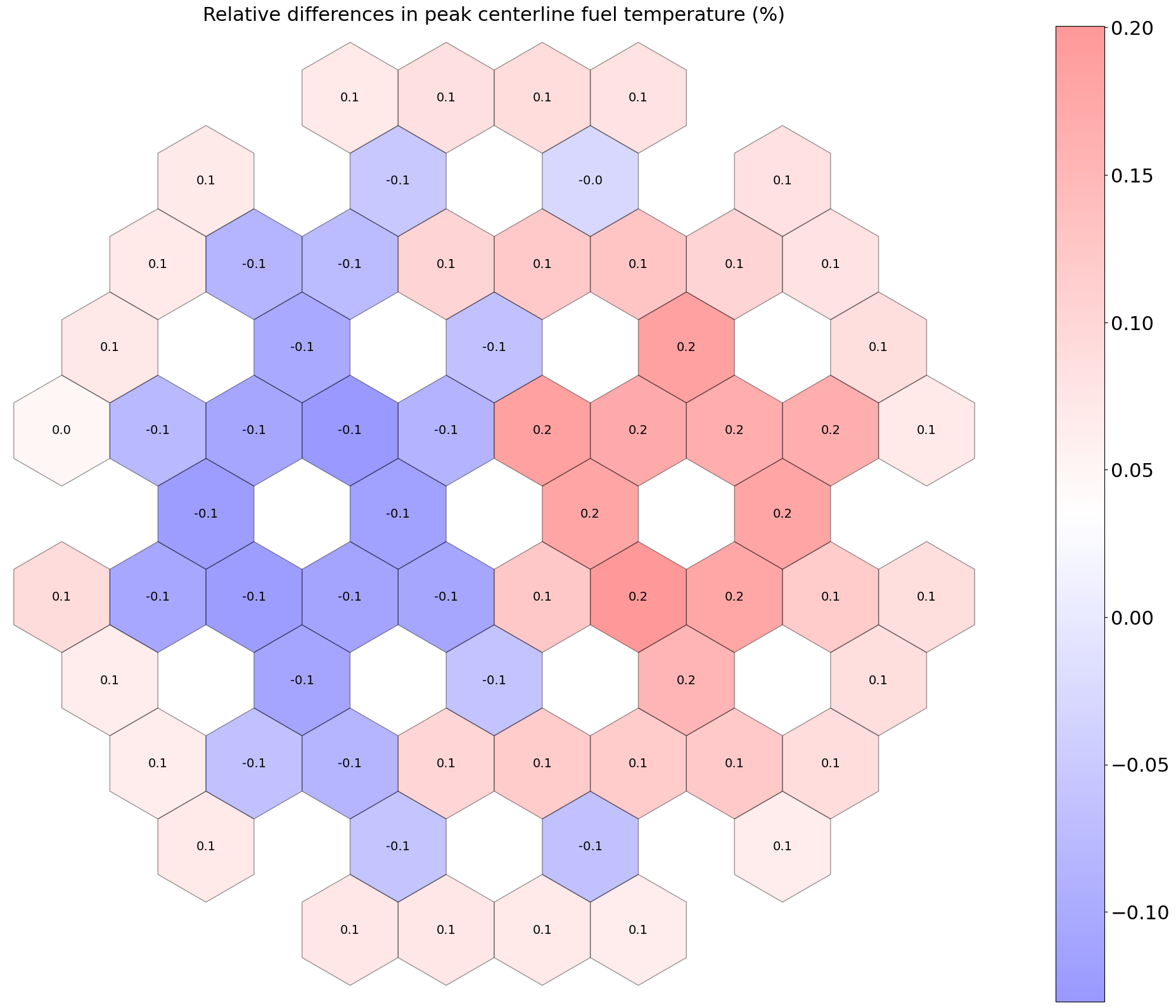
Figure 16: Relative differences in peak fuel temperatures, one-way vs tight coupling (%).