GPBR200 Equilibrium Core Neutronics with Griffin
Contact: Zachary M. Prince, [email protected]
Model link: GPBR200 Griffin Model
Here the input for the Griffin-related physics (Wang et al., 2025) of the GPBR200 model is presented. These physics include the core-wide neutronics along with the equilibrium-core pebble depletion. This stand-alone input will be modified later in Multiphysics Coupling to account for coupling with TH and pebble thermomechanics. The details of neutronics and depletion aspects of this model is presented in Prince et al. (2024); as such, this exposition will focus on explaining specific aspects of the input file.
Input File Variables and Global Parameters
Convenient input file variables are defined in the input for several reasons: defining a single input value to be used in multiple blocks, traceability in how certain values are computed, and defining "perturbable" values (which becomes evident in the sensitivity analysis).
The first set of input file variables are pretty self-evident and utilized ubiquitously through all the physics of PBR models.
# Power ------------------------------------------------------------------------
total_power = 200.0e+6 # Total reactor Power (W)

# Initial values ---------------------------------------------------------------
initial_temperature = 900.0 # (K)

# Geometry ---------------------------------------------------------------------
pbed_porosity = 0.39
pbed_top = 11.3354 # Absolute height of the core top in the model (m).The second set of values involve the geometry of the TRISO particles and the pebble they are embedded in. The values here, particularly the triso_number, are used for computing the initial heavy metal mass; mainly for burnup conversion: MWd/kgHM J/cm3.
# Pebble Geometry --------------------------------------------------------------
pebble_radius = 3.0e-2 # pebble radius (m)
pebble_shell_thickness = 5.0e-03 # pebble fuel free zone thickness (graphite shell) (m)
pebble_volume = '${fparse 4/3*pi*pebble_radius^3}' # volume of the pebble (m3)
pebble_core_volume = '${fparse 4/3*pi*(pebble_radius-pebble_shell_thickness)^3}' # volume of the pebble occupied by TRISO (m3)
kernel_radius = 2.1250e-04 # kernel particle radius (m)
kernel_volume = '${fparse 4/3*pi*kernel_radius^3}' # volume of the kernel (m3)
buffer_thickness = 1.00e-04 # Thickness of buffer (m)
buffer_radius = '${fparse kernel_radius + buffer_thickness}' # Outer radius of buffer (m)
ipyc_thickness = 4.00e-05 # Thickness of IPyC (m)
ipyc_radius = '${fparse buffer_radius + ipyc_thickness}' # Outer radius of IPyC (m)
sic_thickness = 3.50e-05 # Thickness of SiC (m)
sic_radius = '${fparse ipyc_radius + sic_thickness}' # Outer radius of SiC (m)
opyc_thickness = 4.00e-05 # Thickness of OPyC (m)
opyc_radius = '${fparse sic_radius + opyc_thickness}' # Outer radius of OPyC (m)
triso_volume = '${fparse 4/3*pi*opyc_radius^3}' # volume of the particle (m3)
filling_factor = 0.0934404551647307 # Particle filling factor
triso_number = '${fparse pebble_core_volume * filling_factor / triso_volume}' # number of TRISO particle in a pebble (//)The third set of values involve computing initial nuclide concentrations based on fuel enrichment and kernel density. This allows for simple manipulation of these quantities, which the input will automatically convert to values necessary for object parameters.
# Compositions -----------------------------------------------------------------
enrichment = 0.155 # Enrichment in weight fraction
rho_kernel_UCO = 10.4 # Density of UCO (g/cm3)
ACU = 0.3920 # Carbon to Uranium atom ratio in UCO
AOU = 1.4280 # Oxygen to Uranium atom ratio in UCO

MU235 = 235.043929918 # Molar density of U235 (g/mol)
MU238 = 238.050788247 # Molar density of U238 (g/mol)
MC = 12.010735897 # Molar density of Carbon (g/mol)
MO = 15.994914620 # Molar density of Oxygen (g/mol)
enrichment_n = '${fparse enrichment/MU235 / (enrichment/MU235 + (1-enrichment)/MU238)}' # Enrichment in nuclide fration
MUCO = '${fparse MU235*enrichment_n + MU238*(1-enrichment_n) + MC*ACU + MO*AOU}' # UCO molar density (g/mol)
rhon_kernel_UCO = '${fparse rho_kernel_UCO / MUCO * 0.6022140}' # Molar density of UCO (atom/b/cm)

# Kernel number densities (n/b/cm)
rhon_kernel_U235 = '${fparse rhon_kernel_UCO * enrichment_n}'
rhon_kernel_U238 = '${fparse rhon_kernel_UCO * (1 - enrichment_n)}'
rhon_kernel_C = '${fparse rhon_kernel_UCO * ACU}'
rhon_kernel_O = '${fparse rhon_kernel_UCO * AOU}'

# Fractions of pebble volume
kernel_fraction = '${fparse kernel_volume * triso_number / pebble_volume}'

# Pebble volume densities (atoms/b/cm)
rhon_U235 = '${fparse rhon_kernel_U235 * kernel_fraction}'
rhon_U238 = '${fparse rhon_kernel_U238 * kernel_fraction}'For the same purposes, the next set of values define values involved with defining the pebble cycling scheme.
# Parameters describing pebble cycling -----------------------------------------
pebble_unloading_rate = '${fparse 1.5/60}' # pebbles per minute / seconds per minute.
burnup_limit_weight = 147.6 # MWd / kg
rho_U = '${fparse (rhon_U235*MU235 + rhon_U238*MU238) * 1.660539}' # Density of uranium in pebble volume (g/cm3)
burnup_conversion = '${fparse 1e9*3600*24*rho_U}' # Conversion from MWd/kg -> J/m3Finally, there are a relatively large number of blocks in the mesh, so input file variables are defined to promote clarity on where variables, kernels, etc. are acting.
# Blocks -----------------------------------------------------------------------
fuel_blocks = '5 6 7 8 9'
cns_disch_blocks = '14'
upref_blocks = '3 16'
upcav_blocks = '4'
lowref_blocks = '10 11 12 13'
crs_blocks = '17 22'
rdref_blocks = '1 2 15'
rpv_blocks = '18 19 20 21'
ref_blocks = '${cns_disch_blocks} ${upref_blocks}
              ${lowref_blocks}
              ${rdref_blocks}'

# ==============================================================================Global parameters are also useful for propagating a certain parameter shared across many objects. Here, is_meter is used to tell Griffin objects that the mesh units are in meters (versus centimeters) for proper conversion of cross-section values.
[GlobalParams]
  is_meter = true
[]Mesh
The mesh is retained as an Exodus file in the model directory. This mesh contains several extra element ids that are used to describe the materials and the streamlines of the pebble flow, shown in Figure 1. As such, the parameter exodus_extra_element_integers needs to be specified to load this data. Additionally, the 2D geometry is axisymmetric, which is communicated to MOOSE via the coord_type parameter and the rotation axis is specified by the rz_coord_axis parameter.
[Mesh]
  [pebble_bed]
    type = FileMeshGenerator
    file = ../data/streamline_mesh_in.e
    exodus_extra_element_integers = 'pebble_streamline_id pebble_streamline_layer_id material_id'
  []
  coord_type = RZ
  rz_coord_axis = Y
[]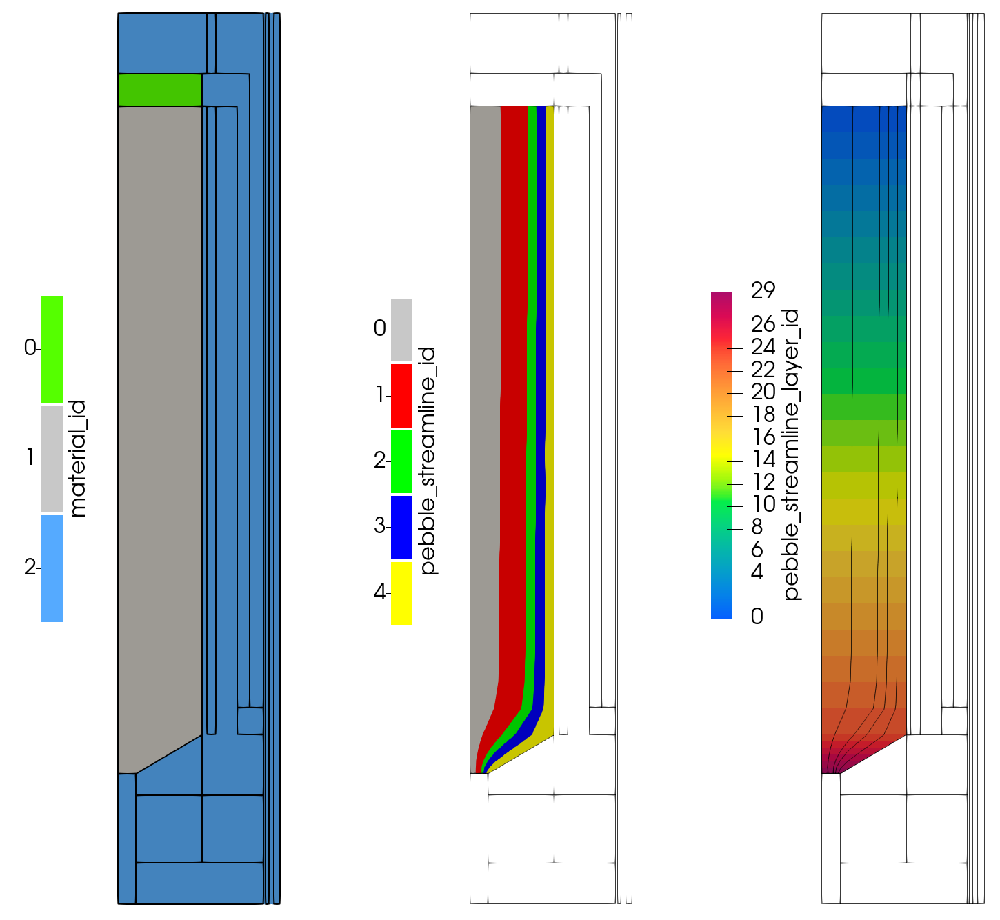
Figure 1: GPBR200 extra element IDs in mesh.
The material_ids represent the three regions where separate cross-section sets were generated: one for the core (fuel) region, reflector (non-fuel) region, and one specific for the upper cavity (void region). The pebble_streamline_ids represent streamlines where pebbles flow down, but don't cross into other streamlines. The pebble_streamline_layer_ids are used to describe the direction of pebble flow within the streamline, flowing from the smallest ID (inlet) to largest (discharge).
Auxiliary Variables
The AuxVariables in this input define the solid temperature distribution in the core and the porosity of the pebble-bed core. The solid temperature, T_solid, is used by Griffin's material system to interpolate cross sections based on the current state of the reactor. Without coupling, this variables is arguably unnecessary; however, when coupling later, this temperature will be filled by the thermal hydraulics simulation. The porosity is also used by Griffin's material system to appropriately compute nuclide concentrations for macroscopic cross-section generation and nuclide advection from pebble flow. This quantity is required by Griffin to be a variable.
[AuxVariables]
  # Temperatures.
  [T_solid]
    family = MONOMIAL
    order = CONSTANT
    initial_condition = ${initial_temperature}
    block = '${fuel_blocks} ${ref_blocks} ${crs_blocks} ${rpv_blocks}' # Everything but upper cavity
  []

  # Porosity
  [porosity]
    family = MONOMIAL
    order = CONSTANT
    block = '${fuel_blocks}'
    initial_condition = ${pbed_porosity}
  []
[]Materials
There are four regions in the geometry that are treated uniquely by Griffin materials: the reflector, control rod, upper cavity, and core.
The reflector region utilizes CoupledFeedbackNeutronicsMaterial, which has constant nuclide concentrations and couples T_solid as its tmod grid variable.
[Materials]
  [reflector]
    type = CoupledFeedbackNeutronicsMaterial
    library_file = '../data/gpbr200_microxs.xml'
    library_name = 'gpbr200_microxs'
    grid_names = 'tmod'
    grid_variables = 'T_solid'
    isotopes = 'Graphite'
    densities = '8.82418e-2'
    plus = true
    material_id = 2
    diffusion_coefficient_scheme = local
    block = '${ref_blocks}'
  []
[]The control rod region utilizes CoupledFeedbackRoddedNeutronicsMaterial, which is similar to the reflector region strategy, except the nuclide concentration is varied spatially according to a function defining the front of the control rod. The insertion depth of the control rod in this example was chosen such that the multiphysics simulation results in a close to unity.
[Materials]
  [crs]
    type = CoupledFeedbackRoddedNeutronicsMaterial
    block = '${crs_blocks}'
    library_file = '../data/gpbr200_microxs.xml'
    library_name = 'gpbr200_microxs'
    grid_names = 'tmod'
    grid_variables = 'T_solid'

    isotopes = ' Graphite;
                 Graphite   B10        B11;
                 Graphite'
    densities = '8.82418e-2
                 7.1628E-02 8.9463E-03  2.2229E-03
                 8.82418e-2'

    rod_segment_length = 1e3
    front_position_function = 'cr_front'
    segment_material_ids = '2 2 2'
    rod_withdrawn_direction = 'y'
    average_segment_id = segment_id
  []
[]

[Functions]
  # Function describing CR depth
  [cr_depth]
    type = ConstantFunction
    value = 1.747 # Range of control rod insertion: -1.318 -> 8.93
  []
  # Offset from reactor reference frame
  [cr_front]
    type = ParsedFunction
    expression = 'top - cr_depth'
    symbol_names = 'top cr_depth'
    symbol_values = '${pbed_top} cr_depth'
  []
[]The upper cavity utilizes a special cross-section set since the region is essentially void, which would otherwise be troublesome for the diffusion approximation being used for the neutronics.
[Materials]
  [cavity]
    type = ConstantNeutronicsMaterial
    block = '${upcav_blocks}'
    fromFile = true
    library_file = '../data/gpbr200_void.xml'
    material_id = 10
  []
[]Defining the nuclide concentration in the core region directly is quite complicated, even at its initial state. Therefore, Griffin's Compositions system is used to build up particle-packed pebble. The resulting composition is communicated to the depletion system (explained in the next section) to build the "depletable" materials for the core region.
[Compositions]
  [uco]
    type = IsotopeComposition
    density_type = atomic
    isotope_densities = '
      U235 ${rhon_kernel_U235}
      U238 ${rhon_kernel_U238}
      C12 ${rhon_kernel_C}
      O16 ${rhon_kernel_O}
    '
  []
  [buffer]
    type = IsotopeComposition
    density_type = atomic
    isotope_densities = 'Graphite 5.26466317651E-02'
  []
  [PyC]
    type = IsotopeComposition
    density_type = atomic
    isotope_densities = 'Graphite 9.52653336702E-02'
  []
  [SiC]
    type = IsotopeComposition
    density_type = atomic
    isotope_densities = '
      SI28 4.43270697709E-02
      SI29 2.25082086520E-03
      SI30 1.48375772443E-03
      C12  4.80616002990E-02
    '
  []
  [matrix]
    type = IsotopeComposition
    density_type = atomic
    isotope_densities = 'Graphite 8.67415932892E-02'
  []
  [triso]
    type = Triso
    compositions = 'uco buffer PyC SiC PyC'
    radii = '${kernel_radius} ${buffer_radius} ${ipyc_radius} ${sic_radius} ${opyc_radius}'
  []
  [triso_fill]
    type = StochasticComposition
    background_composition = matrix
    packing_fractions = ${filling_factor}
    triso_particles = triso
  []
  [pebble]
    type = Pebble
    compositions = 'triso_fill matrix'
    radii = '${fparse pebble_radius - pebble_shell_thickness} ${pebble_radius}'
  []
[]Pebble Depletion
The PebbleDepletion syntax in Griffin enables the multiscale approach Griffin utilizes to perform pebble advection and cycling in the core. This syntax triggers a MOOSE action that builds postprocessors, auxiliary variables/kernels, materials, and user objects that:
Perform power scaling and power density evaluation
Compute macroscopic cross sections for the neutronics solve
Perform the coupled pebble advection and depletion simulation
The first set of parameters specify options related to power scaling and computation of power density. integrated_power_postprocessor and power_density_variable are simply names to give postprocessor and aux-variables, to be consumed by other objects. The family and order are specified to match the power density variable eventually used by the thermal-hydraulics physics.
The second set of parameters relate to microscopic cross section specification, including the XML library used for fueled region, grid variable names for coupled physics, and fixed grid variable values, which will be adjusted for eventual input perturbation in the stochastic analysis. Similarly, the third set of variables specify the XML decay and transmutation data for performing depletion calculations.
The fourth set, namely n_fresh_pebble_types and fresh_pebble_compositions, specify the fresh pebble composition. Since this is an equilibrium-core simulation, there is only one "type" of pebble introduced into the core. Depleted pebbles are recycled through the core, but these do not constitute a different type of pebble. The fifth set of parameters specify the density of pebbles and burnup discretization for the pebble depletion, which here is 12 bins, where the last bin starts at 196.8 MWd/kgHM (converted to J/cm3 using fparse).
The DepletionScheme block primarily specifies that an equilibrium-core simulation is to be performed. The parameters in this block include specifications on how the pebbles spatially traverse the core. Where pebble_unloading_rate specifies the rate at which pebbles enter/exit the core, pebble_flow_rate_distribution is the fraction of this rate for each streamline (according to the pebble_streamline_id element ID), and burnup_limit specifies the minimum burnup a pebble must reach upon exiting the core to be discarded for a fresh pebble. sweep_tol and sweep_max_iterations are solver parameters for the advection-depletion system. exodus_streamline_output can be set to true if a full profile of isotopic concentrations throughout the core is desired at output.
[PebbleDepletion]
  block = '${fuel_blocks}'

  # Power.
  power = ${total_power}
  integrated_power_postprocessor = total_power
  power_density_variable = total_power_density
  family = MONOMIAL
  order = CONSTANT

  # Cross section data.
  library_file = '../data/gpbr200_microxs.xml'
  library_name = 'gpbr200_microxs'
  fuel_temperature_grid_name = 'tfuel'
  moderator_temperature_grid_name = 'tmod'
  burnup_grid_name = 'burnup'
  constant_grid_values = 'kernrad ${fparse kernel_radius * 1000}
                          fillfact ${filling_factor}
                          enrich ${enrichment}'

  # Transmutation data.
  dataset = ISOXML
  isoxml_data_file = '../data/gpbr200_dtl.xml'
  isoxml_lib_name = 'gpbr200_dtl'
  # Some of the branching ratios in the DTL are unphysical, which Griffin will
  # throw a warning for unless this is specified.
  dtl_physicality = 'SILENT'

  # Isotopic options
  n_fresh_pebble_types = 1
  fresh_pebble_compositions = 'pebble'

  # Pebble options
  porosity_name = porosity
  maximum_burnup = '${fparse 196.8 * burnup_conversion}'
  num_burnup_bins = 12

  # Tabulation data.
  initial_moderator_temperature = '${initial_temperature}'
  initial_fuel_temperature = '${initial_temperature}'

  [DepletionScheme]
    type = ConstantStreamlineEquilibrium

    # Streamline definition
    major_streamline_axis = y

    # Pebble options
    pebble_unloading_rate = ${pebble_unloading_rate}
    pebble_flow_rate_distribution = '0.12919675255653704 0.3237409742330389 0.16364127845178317 0.1970045449547337 0.1864164498039072'
    pebble_diameter = '${fparse pebble_radius * 2.0}'
    burnup_limit = '${fparse burnup_limit_weight * burnup_conversion}'

    # Solver parameters
    sweep_tol = 1e-8
    sweep_max_iterations = 20

    # Output
    exodus_streamline_output = false
  []

  diffusion_coefficient_scheme = local
[]Transport Systems
The last portion of the input describing the physics is the TransportSystems block. This block defines what form of the transport equation is being solved, including: type of particle (neutron), equation type (eigenvalue/criticality), number of energy groups (9), spatial and angular discretization (CFEM-Diffusion), and number of delay neutron precursors (6). Additionally, the boundary conditions are defined here; note that even reflecting conditions need to be defined with a diffusion system. Finally, which portions of the Jacobian should be computed are also specified; it is highly recommended to include all portions (scattering and fission) for diffusion systems.
[TransportSystems]
  particle = neutron
  equation_type = eigenvalue
  G = 9
  ReflectingBoundary = 'rinner'
  VacuumBoundary = 'rtop rbottom router'
  [diff]
    scheme = CFEM-Diffusion
    family = LAGRANGE
    order = FIRST
    n_delay_groups = 6
    assemble_scattering_jacobian = true
    assemble_fission_jacobian = true
    block = '${fuel_blocks} ${upcav_blocks} ${ref_blocks} ${crs_blocks}' # Excluding RPV and Barrel
  []
[]Executioner
The final relevant block of the neutronics input is the Executioner. Here, the Eigenvalue solver is specified using the PJFNKMO method. This method, along with linear and nonlinear parameters specified are common for neutron diffusion simulations. Since the simulation is coupling neutron diffusion with pebble depletion, the input specifies parameters enabling fixed-point iteration. The convergence of this iteration considers the , or eigenvalue, convergence as its metric.
[Executioner]
  type = Eigenvalue
  solve_type = 'PJFNKMO'
  constant_matrices = true
  petsc_options_iname = '-pc_type -pc_hypre_type -ksp_gmres_restart '
  petsc_options_value = 'hypre boomeramg 100'
  line_search = none

  # Linear/nonlinear iterations.
  l_max_its = 100
  l_tol = 1e-3

  nl_max_its = 50
  nl_rel_tol = 1e-7
  nl_abs_tol = 1e-9

  # Fixed point iterations.
  fixed_point_min_its = 15
  fixed_point_max_its = 200
  custom_pp = eigenvalue
  custom_abs_tol = 5e-5
  custom_rel_tol = 1e-50
  disable_fixed_point_residual_norm_check = true

  # Power iterations.
  free_power_iterations = 4
  extra_power_iterations = 20
[]Results
The input can be run using a griffin-opt or blue_crab-opt executable:
mpiexec -n 8 blue_crab-opt -i gpbr200_ss_gfnk_reactor.i
The resulting eigenvalue is approximately 1.01496. Additionally, Figure 2 shows the resulting power density, fast scalar flux, and thermal flux.
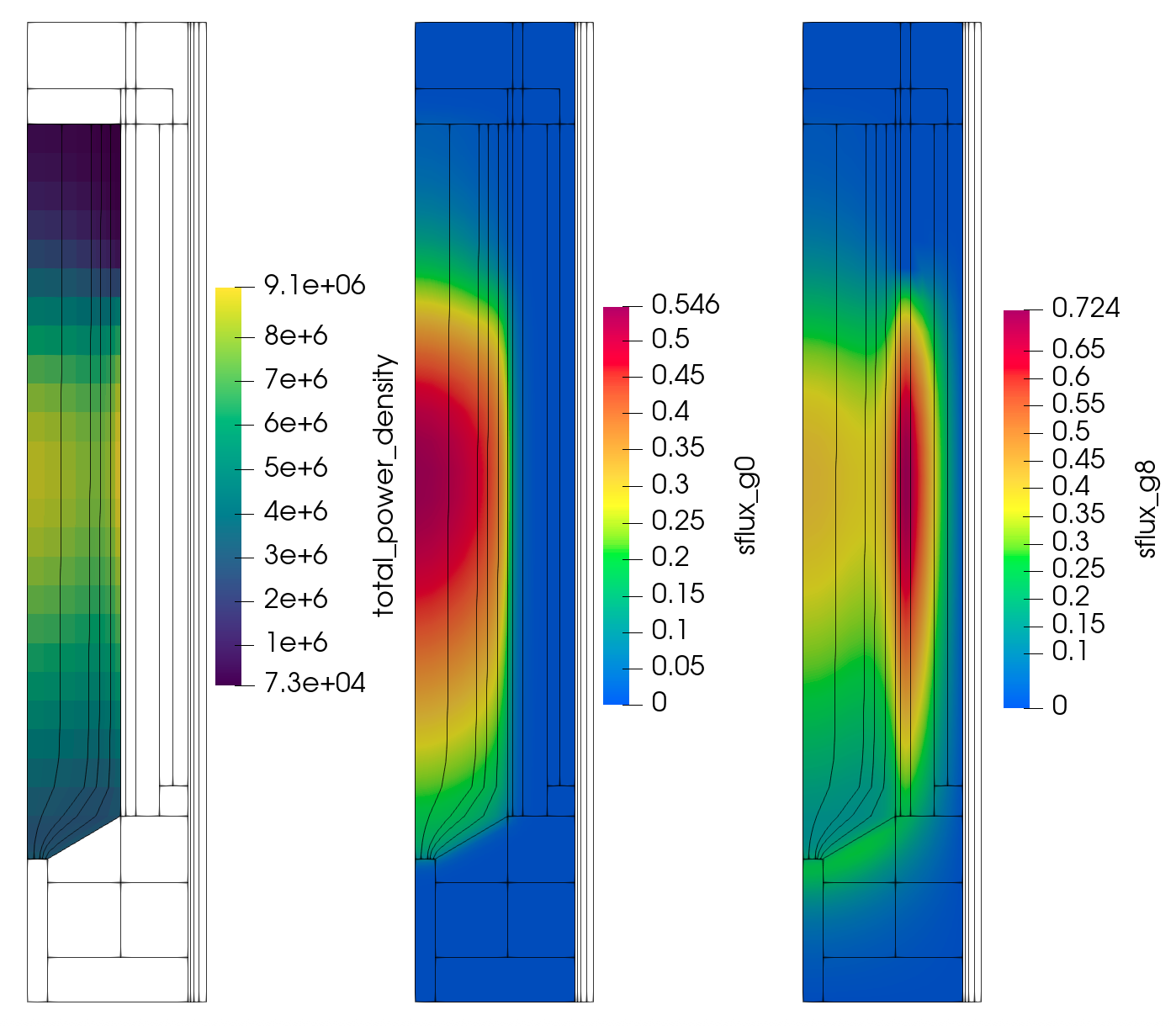
Figure 2: GPBR200 neutronics-only selected field variables
The use of 8 processors in the command listing is somewhat arbitrary, Table 1 shows the expected scaling performance.
Table 1: Run times for GPBR200 neutronics-only input with varying number of processors
| Processors | Run-time (min) |
|---|---|
| 1 | 7.3 |
| 2 | 4.7 |
| 4 | 3.7 |
| 8 | 2.6 |
| 16 | 1.9 |
| 32 | 1.4 |
References
- Zachary M. Prince, Paolo Balestra, Javier Ortensi, Sebastian Schunert, Olin Calvin, Joshua T. Hanophy, Kun Mo, and Gerhard Strydom.
Sensitivity analysis, surrogate modeling, and optimization of pebble-bed reactors considering normal and accident conditions.
Nuclear Engineering and Design, 428:113466, 2024.
doi:https://doi.org/10.1016/j.nucengdes.2024.113466.[BibTeX]
@article{prince2024Sensitivity, author = "Prince, Zachary M. and Balestra, Paolo and Ortensi, Javier and Schunert, Sebastian and Calvin, Olin and Hanophy, Joshua T. and Mo, Kun and Strydom, Gerhard", title = "Sensitivity analysis, surrogate modeling, and optimization of pebble-bed reactors considering normal and accident conditions", journal = "Nuclear Engineering and Design", volume = "428", pages = "113466", year = "2024", issn = "0029-5493", doi = "https://doi.org/10.1016/j.nucengdes.2024.113466" } - Yaqi Wang, Zachary M. Prince, Hansol Park, Olin W. Calvin, Namjae Choi, Yeon Sang Jung, Sebastian Schunert, Shikhar Kumar, Joshua T. Hanophy, Vincent M. Labouré, Changho Lee, Javier Ortensi, Logan H. Harbour, and Jackson R. Harter.
Griffin: a moose-based reactor physics application for multiphysics simulation of advanced nuclear reactors.
Annals of Nuclear Energy, 211:110917, 2025.
URL: https://www.sciencedirect.com/science/article/pii/S0306454924005802, doi:https://doi.org/10.1016/j.anucene.2024.110917.[BibTeX]
@article{wang2025Griffin,
    author = "Wang, Yaqi and Prince, Zachary M. and Park, Hansol and Calvin, Olin W. and Choi, Namjae and Jung, Yeon Sang and Schunert, Sebastian and Kumar, Shikhar and Hanophy, Joshua T. and Labouré, Vincent M. and Lee, Changho and Ortensi, Javier and Harbour, Logan H. and Harter, Jackson R.",
    title = "Griffin: A MOOSE-based reactor physics application for multiphysics simulation of advanced nuclear reactors",
    journal = "Annals of Nuclear Energy",
    volume = "211",
    pages = "110917",
    year = "2025",
    issn = "0306-4549",
    doi = "https://doi.org/10.1016/j.anucene.2024.110917",
    url = "https://www.sciencedirect.com/science/article/pii/S0306454924005802",
    keywords = "Griffin, MOOSE, Radiation transport, Multiphysics, Reactor analysis"
}
(htgr/gpbr200/core_neutronics/gpbr200_ss_gfnk_reactor.i)
# ==============================================================================
# Model description:
# Equilibrium core neutronics model coupled with TH and pebble temperature
# models.
# ------------------------------------------------------------------------------
# Idaho Falls, INL, April 4, 2022 11:03 AM
# Author(s)(name alph): David Reger, Dr. Javier Ortensi, Dr. Paolo Balestra,
#   Dr. Ryan Stewart, Dr. Sebastian Schunert, Dr. Zachary Prince.
# ==============================================================================
# MODEL PARAMETERS
# ==============================================================================

# Power ------------------------------------------------------------------------
total_power = 200.0e+6 # Total reactor Power (W)

# Initial values ---------------------------------------------------------------
initial_temperature = 900.0 # (K)

# Geometry ---------------------------------------------------------------------
pbed_porosity = 0.39
pbed_top = 11.3354 # Absolute height of the core top in the model (m).

# Pebble Geometry --------------------------------------------------------------
pebble_radius = 3.0e-2 # pebble radius (m)
pebble_shell_thickness = 5.0e-03 # pebble fuel free zone thickness (graphite shell) (m)
pebble_volume = '${fparse 4/3*pi*pebble_radius^3}' # volume of the pebble (m3)
pebble_core_volume = '${fparse 4/3*pi*(pebble_radius-pebble_shell_thickness)^3}' # volume of the pebble occupied by TRISO (m3)
kernel_radius = 2.1250e-04 # kernel particle radius (m)
kernel_volume = '${fparse 4/3*pi*kernel_radius^3}' # volume of the kernel (m3)
buffer_thickness = 1.00e-04 # Thickness of buffer (m)
buffer_radius = '${fparse kernel_radius + buffer_thickness}' # Outer radius of buffer (m)
ipyc_thickness = 4.00e-05 # Thickness of IPyC (m)
ipyc_radius = '${fparse buffer_radius + ipyc_thickness}' # Outer radius of IPyC (m)
sic_thickness = 3.50e-05 # Thickness of SiC (m)
sic_radius = '${fparse ipyc_radius + sic_thickness}' # Outer radius of SiC (m)
opyc_thickness = 4.00e-05 # Thickness of OPyC (m)
opyc_radius = '${fparse sic_radius + opyc_thickness}' # Outer radius of OPyC (m)
triso_volume = '${fparse 4/3*pi*opyc_radius^3}' # volume of the particle (m3)
filling_factor = 0.0934404551647307 # Particle filling factor
triso_number = '${fparse pebble_core_volume * filling_factor / triso_volume}' # number of TRISO particle in a pebble (//)

# Compositions -----------------------------------------------------------------
enrichment = 0.155 # Enrichment in weight fraction
rho_kernel_UCO = 10.4 # Density of UCO (g/cm3)
ACU = 0.3920 # Carbon to Uranium atom ratio in UCO
AOU = 1.4280 # Oxygen to Uranium atom ratio in UCO

MU235 = 235.043929918 # Molar density of U235 (g/mol)
MU238 = 238.050788247 # Molar density of U238 (g/mol)
MC = 12.010735897 # Molar density of Carbon (g/mol)
MO = 15.994914620 # Molar density of Oxygen (g/mol)
enrichment_n = '${fparse enrichment/MU235 / (enrichment/MU235 + (1-enrichment)/MU238)}' # Enrichment in nuclide fration
MUCO = '${fparse MU235*enrichment_n + MU238*(1-enrichment_n) + MC*ACU + MO*AOU}' # UCO molar density (g/mol)
rhon_kernel_UCO = '${fparse rho_kernel_UCO / MUCO * 0.6022140}' # Molar density of UCO (atom/b/cm)

# Kernel number densities (n/b/cm)
rhon_kernel_U235 = '${fparse rhon_kernel_UCO * enrichment_n}'
rhon_kernel_U238 = '${fparse rhon_kernel_UCO * (1 - enrichment_n)}'
rhon_kernel_C = '${fparse rhon_kernel_UCO * ACU}'
rhon_kernel_O = '${fparse rhon_kernel_UCO * AOU}'

# Fractions of pebble volume
kernel_fraction = '${fparse kernel_volume * triso_number / pebble_volume}'

# Pebble volume densities (atoms/b/cm)
rhon_U235 = '${fparse rhon_kernel_U235 * kernel_fraction}'
rhon_U238 = '${fparse rhon_kernel_U238 * kernel_fraction}'

# Parameters describing pebble cycling -----------------------------------------
pebble_unloading_rate = '${fparse 1.5/60}' # pebbles per minute / seconds per minute.
burnup_limit_weight = 147.6 # MWd / kg
rho_U = '${fparse (rhon_U235*MU235 + rhon_U238*MU238) * 1.660539}' # Density of uranium in pebble volume (g/cm3)
burnup_conversion = '${fparse 1e9*3600*24*rho_U}' # Conversion from MWd/kg -> J/m3

# Blocks -----------------------------------------------------------------------
fuel_blocks = '5 6 7 8 9'
cns_disch_blocks = '14'
upref_blocks = '3 16'
upcav_blocks = '4'
lowref_blocks = '10 11 12 13'
crs_blocks = '17 22'
rdref_blocks = '1 2 15'
rpv_blocks = '18 19 20 21'
ref_blocks = '${cns_disch_blocks} ${upref_blocks}
              ${lowref_blocks}
              ${rdref_blocks}'

# ==============================================================================
# GLOBAL PARAMETERS
# ==============================================================================
[GlobalParams]
  is_meter = true
[]

# ==============================================================================
# GEOMETRY AND MESH
# ==============================================================================
[Mesh]
  [pebble_bed]
    type = FileMeshGenerator
    file = ../data/streamline_mesh_in.e
    exodus_extra_element_integers = 'pebble_streamline_id pebble_streamline_layer_id material_id'
  []
  coord_type = RZ
  rz_coord_axis = Y
[]

# ==============================================================================
# AUXVARIABLES AND AUXKERNELS
# ==============================================================================
[AuxVariables]
  # Temperatures.
  [T_solid]
    family = MONOMIAL
    order = CONSTANT
    initial_condition = ${initial_temperature}
    block = '${fuel_blocks} ${ref_blocks} ${crs_blocks} ${rpv_blocks}' # Everything but upper cavity
  []

  # Porosity
  [porosity]
    family = MONOMIAL
    order = CONSTANT
    block = '${fuel_blocks}'
    initial_condition = ${pbed_porosity}
  []
[]

# ==============================================================================
# MATERIALS
# ==============================================================================
[Materials]
  [reflector]
    type = CoupledFeedbackNeutronicsMaterial
    library_file = '../data/gpbr200_microxs.xml'
    library_name = 'gpbr200_microxs'
    grid_names = 'tmod'
    grid_variables = 'T_solid'
    isotopes = 'Graphite'
    densities = '8.82418e-2'
    plus = true
    material_id = 2
    diffusion_coefficient_scheme = local
    block = '${ref_blocks}'
  []
  [crs]
    type = CoupledFeedbackRoddedNeutronicsMaterial
    block = '${crs_blocks}'
    library_file = '../data/gpbr200_microxs.xml'
    library_name = 'gpbr200_microxs'
    grid_names = 'tmod'
    grid_variables = 'T_solid'

    isotopes = ' Graphite;
                 Graphite   B10        B11;
                 Graphite'
    densities = '8.82418e-2
                 7.1628E-02 8.9463E-03  2.2229E-03
                 8.82418e-2'

    rod_segment_length = 1e3
    front_position_function = 'cr_front'
    segment_material_ids = '2 2 2'
    rod_withdrawn_direction = 'y'
    average_segment_id = segment_id
  []
  [cavity]
    type = ConstantNeutronicsMaterial
    block = '${upcav_blocks}'
    fromFile = true
    library_file = '../data/gpbr200_void.xml'
    material_id = 10
  []
[]

[Functions]
  # Function describing CR depth
  [cr_depth]
    type = ConstantFunction
    value = 1.747 # Range of control rod insertion: -1.318 -> 8.93
  []
  # Offset from reactor reference frame
  [cr_front]
    type = ParsedFunction
    expression = 'top - cr_depth'
    symbol_names = 'top cr_depth'
    symbol_values = '${pbed_top} cr_depth'
  []
[]

[Compositions]
  [uco]
    type = IsotopeComposition
    density_type = atomic
    isotope_densities = '
      U235 ${rhon_kernel_U235}
      U238 ${rhon_kernel_U238}
      C12 ${rhon_kernel_C}
      O16 ${rhon_kernel_O}
    '
  []
  [buffer]
    type = IsotopeComposition
    density_type = atomic
    isotope_densities = 'Graphite 5.26466317651E-02'
  []
  [PyC]
    type = IsotopeComposition
    density_type = atomic
    isotope_densities = 'Graphite 9.52653336702E-02'
  []
  [SiC]
    type = IsotopeComposition
    density_type = atomic
    isotope_densities = '
      SI28 4.43270697709E-02
      SI29 2.25082086520E-03
      SI30 1.48375772443E-03
      C12  4.80616002990E-02
    '
  []
  [matrix]
    type = IsotopeComposition
    density_type = atomic
    isotope_densities = 'Graphite 8.67415932892E-02'
  []
  [triso]
    type = Triso
    compositions = 'uco buffer PyC SiC PyC'
    radii = '${kernel_radius} ${buffer_radius} ${ipyc_radius} ${sic_radius} ${opyc_radius}'
  []
  [triso_fill]
    type = StochasticComposition
    background_composition = matrix
    packing_fractions = ${filling_factor}
    triso_particles = triso
  []
  [pebble]
    type = Pebble
    compositions = 'triso_fill matrix'
    radii = '${fparse pebble_radius - pebble_shell_thickness} ${pebble_radius}'
  []
[]

# ==============================================================================
# PEBBLE DEPLETION
# ==============================================================================
[PebbleDepletion]
  block = '${fuel_blocks}'

  # Power.
  power = ${total_power}
  integrated_power_postprocessor = total_power
  power_density_variable = total_power_density
  family = MONOMIAL
  order = CONSTANT

  # Cross section data.
  library_file = '../data/gpbr200_microxs.xml'
  library_name = 'gpbr200_microxs'
  fuel_temperature_grid_name = 'tfuel'
  moderator_temperature_grid_name = 'tmod'
  burnup_grid_name = 'burnup'
  constant_grid_values = 'kernrad ${fparse kernel_radius * 1000}
                          fillfact ${filling_factor}
                          enrich ${enrichment}'

  # Transmutation data.
  dataset = ISOXML
  isoxml_data_file = '../data/gpbr200_dtl.xml'
  isoxml_lib_name = 'gpbr200_dtl'
  # Some of the branching ratios in the DTL are unphysical, which Griffin will
  # throw a warning for unless this is specified.
  dtl_physicality = 'SILENT'

  # Isotopic options
  n_fresh_pebble_types = 1
  fresh_pebble_compositions = 'pebble'

  # Pebble options
  porosity_name = porosity
  maximum_burnup = '${fparse 196.8 * burnup_conversion}'
  num_burnup_bins = 12

  # Tabulation data.
  initial_moderator_temperature = '${initial_temperature}'
  initial_fuel_temperature = '${initial_temperature}'

  [DepletionScheme]
    type = ConstantStreamlineEquilibrium

    # Streamline definition
    major_streamline_axis = y

    # Pebble options
    pebble_unloading_rate = ${pebble_unloading_rate}
    pebble_flow_rate_distribution = '0.12919675255653704 0.3237409742330389 0.16364127845178317 0.1970045449547337 0.1864164498039072'
    pebble_diameter = '${fparse pebble_radius * 2.0}'
    burnup_limit = '${fparse burnup_limit_weight * burnup_conversion}'

    # Solver parameters
    sweep_tol = 1e-8
    sweep_max_iterations = 20

    # Output
    exodus_streamline_output = false
  []

  diffusion_coefficient_scheme = local
[]

# ==============================================================================
# EXECUTION PARAMETERS
# ==============================================================================
[TransportSystems]
  particle = neutron
  equation_type = eigenvalue
  G = 9
  ReflectingBoundary = 'rinner'
  VacuumBoundary = 'rtop rbottom router'
  [diff]
    scheme = CFEM-Diffusion
    family = LAGRANGE
    order = FIRST
    n_delay_groups = 6
    assemble_scattering_jacobian = true
    assemble_fission_jacobian = true
    block = '${fuel_blocks} ${upcav_blocks} ${ref_blocks} ${crs_blocks}' # Excluding RPV and Barrel
  []
[]

[Executioner]
  type = Eigenvalue
  solve_type = 'PJFNKMO'
  constant_matrices = true
  petsc_options_iname = '-pc_type -pc_hypre_type -ksp_gmres_restart '
  petsc_options_value = 'hypre boomeramg 100'
  line_search = none

  # Linear/nonlinear iterations.
  l_max_its = 100
  l_tol = 1e-3

  nl_max_its = 50
  nl_rel_tol = 1e-7
  nl_abs_tol = 1e-9

  # Fixed point iterations.
  fixed_point_min_its = 15
  fixed_point_max_its = 200
  custom_pp = eigenvalue
  custom_abs_tol = 5e-5
  custom_rel_tol = 1e-50
  disable_fixed_point_residual_norm_check = true

  # Power iterations.
  free_power_iterations = 4
  extra_power_iterations = 20
[]

# ==============================================================================
# POSTPROCESSORS DEBUG AND OUTPUTS
# ==============================================================================

[Outputs]
  csv = true
  exodus = true
[]