GPBR200 Design-Space Sensitivity Analysis
Contact: Zachary M. Prince, [email protected]
Model link: GPBR200 Sensitivity Analysis
The MOOSE stochastic tools module (STM) contains utilities and capabilities useful for stochastic simulation of MOOSE-based models (Slaughter et al., 2023). In this exposition, a sensitivity analysis is performed on the GPBR200 equilibrium core model using the STM. This is a analog to the sensitivity analysis performed in Section 3 of Prince et al. (2024). This analysis has four objectives:
Identify design parameters and QoIs (stm_base_sampling.i)
Perform qualitative sensitivity analysis (stm_grid_study.i)
Produce a training dataset (stm_lhs_sampling.i)
Compute global sensitivities (stm_poly_chaos.i)
Parameters and QoIs
Six parameters in the GPBR200 model were chosen to define the design-space and five quantities of interest (QoIs) were chosen for the analysis. The parameters are defined in Table 1 with a lower and upper bound describing their uniform probability distribution, as well as their nominal value for comparison. The QoIs are defined in Table 2 with their nominal values, which are the values as a result of evaluating the model at the parameters' nominal values.
Table 1: Design space for the GPBR200 model.
| Parameter | Nominal Value | Lower Bound | Upper Bound | Unit |
|---|---|---|---|---|
| Kernel radius | 0.2125 | 0.15 | 0.3 | mm |
| Filling factor | 9.34 | 5 | 15 | % |
| Enrichment | 15.5 | 5 | 20 | wt% |
| Feed rate | 1.5 | 1 | 3 | pebbles/min |
| Burnup limit | 147.6 | 131.2 | 164.0 | MWd/kg |
| Total power | 200 | 180 | 220 | MW |
Table 2: Quantities of interest for the GPBR200 model.
| QoI | Nominal Value | Unit |
|---|---|---|
| Eigenvalue | 1.00129 | — |
| Max fuel temperature | 1281 | K |
| Max RPV temperature | 508.5 | K |
| Max pebble power | 2.67 | kW |
| Peaking factor | 2.012 | — |
Modified GPBR200 Model
The fully-coupled GPBR200 equilibrium-core input is largely unchanged from that described in the previous step. The primary difference in the inclusion of postprocessors defining the QoIs and the removal of Outputs.
[Postprocessors]
  # Temperatures
  [Tfuel_max]
    type = ElementExtremeValue
    variable = Tfuel_max
    block = ${fuel_blocks}
  []
  [Trpv_max]
    type = ElementExtremeValue
    variable = T_solid
    block = 21
  []

  # Pebble power
  [ppd_max]
    type = ElementExtremeValue
    variable = ppd_max
    block = ${fuel_blocks}
    outputs = none
  []
  [pebble_power_max]
    type = ScalePostprocessor
    value = ppd_max
    scaling_factor = '${pebble_volume}'
  []

  # Reactor power
  [power_max]
    type = ElementExtremeValue
    variable = total_power_density
    block = ${fuel_blocks}
    outputs = none
  []
  [power_avg]
    type = ElementAverageValue
    variable = total_power_density
    block = ${fuel_blocks}
    outputs = none
  []
  [peaking_factor]
    type = ParsedPostprocessor
    expression = 'power_max / power_avg'
    pp_names = 'power_max power_avg'
  []
[]The other, more minor, modification is in the thermal hydraulics input, where dt_min and error_on_dtmin are specified. This insures that the stochastic simulation doesn't stall on a difficult-to-converge configuration and simply marks the sample as "uncoverged".
 @@ -1,30 +1,32 @@
 [Executioner]
   type = Transient
   solve_type = NEWTON
-  petsc_options_iname = '-pc_type'
-  petsc_options_value = 'lu'
+  petsc_options_iname = '-pc_type -sub_pc_factor_shift_type'
+  petsc_options_value = 'lu       NONZERO'
   line_search = l2

   # Scaling.
   automatic_scaling = true
   off_diagonals_in_auto_scaling = false
   compute_scaling_once = false

   # Tolerances.
   nl_abs_tol = 1e-5
   nl_rel_tol = 1e-6
   nl_max_its = 15

   # Time step control.
   [TimeStepper]
     type = IterationAdaptiveDT
     dt = 2.5e-3
     cutback_factor = 0.5
     growth_factor = 2.00
     optimal_iterations = 8
   []

   # Steady state detection.
   steady_state_detection = true
   steady_state_tolerance = 1e-13
+  error_on_dtmin = false
+  dtmin = 1e-6
[](+ htgr/gpbr200/sensitivity_analysis/gpbr200_ss_phth_reactor.i)
Base Sampling Input
This input defines most of the objects necessary for sampling the GPBR200 model and gathering the QoIs. First, input file variables are specified defining the upper and lower bounds of the design-space parameters.
The parameter bounds and nominal values are defined in the relevant input files of the model:
# Kernel radius (m) ------------------------------------------------------------
kernel_radius_min = 1.5e-4
kernel_radius_max = 3.0e-4

# Filling factor ---------------------------------------------------------------
filling_factor_min = 0.05
filling_factor_max = 0.15

# Enrichment -------------------------------------------------------------------
enrichment_min = 0.05
enrichment_max = 0.2

# Pebble unloading rate (pebbles per second) -----------------------------------
pebble_unloading_rate_min = '${fparse 1.0/60}'
pebble_unloading_rate_max = '${fparse 3.0/60}'

# Burnup limit (MWD/kg) --------------------------------------------------------
burnup_limit_weight_min = 131.2 # MWd / kg
burnup_limit_weight_max = 164 # MWd / kg

# Total power (W) --------------------------------------------------------------
total_power_min = 180e6
total_power_max = 220e6The STM utilizes the MultiApps system to perform the sampling, namely with SamplerFullSolveMultiApp. In this block, the GPBR200 input is specified; along with the sampler defining the parameter values of all the configurations to be sampled (this object will be defined in the next two sections). The mode and min_procs_per_app parameters specify the method in which the multiapps are distributed, i.e. only one app per four processors available are instantiated at time; this minimizes the number of HPC nodes the execution needs to allocate. The ignore_solve_not_converge parameter allows the sampling to continue even if one of the sample's solve fails to converge.
[MultiApps]
  [sub]
    type = SamplerFullSolveMultiApp
    input_files = gpbr200_ss_gfnk_reactor.i
    sampler = sample
    mode = batch-reset
    min_procs_per_app = 4
    ignore_solve_not_converge = true
  []
[]Next, a Controls object is specified, which takes the configurations defined by the sampler and applies them as command-line arguments when instantiating the sub-applications.
[Controls]
  [param]
    type = MultiAppSamplerControl
    sampler = sample
    multi_app = sub
    param_names = 'kernel_radius
                   filling_factor
                   enrichment
                   pebble_unloading_rate
                   burnup_limit_weight
                   total_power'
  []
[]Next, a StochasticMatrix reporter is specified, which serves as a storage object that contains all the parameters and resulting QoIs for each configuration. This eventually gets outputted as a CSV file.
[Reporters]
  [storage]
    type = StochasticMatrix
    sampler = sample
    sampler_column_names = 'kernel_radius
                            filling_factor
                            enrichment
                            pebble_unloading_rate
                            burnup_limit_weight
                            total_power'
    parallel_type = ROOT
  []
[]Finally, a Transfers object is specified for extracting the postprocessors from the sub-applications and filling in the storage reporter.
[Transfers]
  [data]
    type = SamplerReporterTransfer
    from_multi_app = sub
    sampler = sample
    stochastic_reporter = storage
    from_reporter = 'eigenvalue/value
                     Tfuel_max/value
                     Trpv_max/value
                     pebble_power_max/value
                     peaking_factor/value'
  []
[]1D Grid Study
The goal of this input is to perform a qualitative analysis on how each parameter impacts each quantity of interest individually. The method utilizes a Cartesian1D sampler to sample each parameter at 12 equidistant points between their upper and lower bound, while keeping all other parameters the same. The resulting number of samples is .
!include stm_base_sampling.i

# Nominal parameter values -----------------------------------------------------
kernel_radius = 2.1250e-04
filling_factor = 0.0934404551647307 # Particle filling factor
enrichment = 0.155 # Enrichment in weight fraction
pebble_unloading_rate = '${fparse 1.5/60}' # pebbles per minute / seconds per minute.
burnup_limit_weight = 147.6 # MWd / kg
total_power = 200.0e+6 # Total reactor Power (W)

# Grid stepping ----------------------------------------------------------------
ngrid = 12
kernel_radius_step = '${fparse (kernel_radius_max - kernel_radius_min) / (ngrid - 1)}'
filling_factor_step = '${fparse (filling_factor_max - filling_factor_min) / (ngrid - 1)}'
enrichment_step = '${fparse (enrichment_max - enrichment_min) / (ngrid - 1)}'
pebble_unloading_rate_step = '${fparse (pebble_unloading_rate_max - pebble_unloading_rate_min) / (ngrid - 1)}'
burnup_limit_weight_step = '${fparse (burnup_limit_weight_max - burnup_limit_weight_min) / (ngrid - 1)}'
total_power_step = '${fparse (total_power_max - total_power_min) / (ngrid - 1)}'

[Samplers]
  [sample]
    type = Cartesian1D
    nominal_values = '${kernel_radius} ${filling_factor} ${enrichment} ${pebble_unloading_rate} ${burnup_limit_weight} ${total_power}'
    linear_space_items = '${kernel_radius_min} ${kernel_radius_step} ${ngrid}
                          ${filling_factor_min} ${filling_factor_step} ${ngrid}
                          ${enrichment_min} ${enrichment_step} ${ngrid}
                          ${pebble_unloading_rate_min} ${pebble_unloading_rate_step} ${ngrid}
                          ${burnup_limit_weight_min} ${burnup_limit_weight_step} ${ngrid}
                          ${total_power_min} ${total_power_step} ${ngrid}'
    min_procs_per_row = 4
    execute_on = PRE_MULTIAPP_SETUP
  []
[]
Running this input requires the use of a blue_crab-opt executable. Each sample takes an average of 10 min to complete on 4 processors. Figure 1 shows the dependency each parameter has on each QoI. Note that the parameters are scaled based on nominal values and lower and upper bounds.
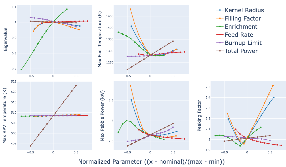
Figure 1: Quantities of interest versus design parameters from performing one-dimensional grid sampling.
Random Sampling
The purpose of this next input is essentially to generate a lot of data. This data will be used in the next section to perform global sensitivity analysis. This is done by specifying a LatinHypercube sampler, which evaluates the parameter Distributions' quantile to generate 10,000 random configurations of the model.
!include stm_base_sampling.i

[Distributions]
  [kr]
    type = Uniform
    lower_bound = ${kernel_radius_min}
    upper_bound = ${kernel_radius_max}
  []
  [ff]
    type = Uniform
    lower_bound = ${filling_factor_min}
    upper_bound = ${filling_factor_max}
  []
  [enrich]
    type = Uniform
    lower_bound = ${enrichment_min}
    upper_bound = ${enrichment_max}
  []
  [pur]
    type = Uniform
    lower_bound = ${pebble_unloading_rate_min}
    upper_bound = ${pebble_unloading_rate_max}
  []
  [bul]
    type = Uniform
    lower_bound = ${burnup_limit_weight_min}
    upper_bound = ${burnup_limit_weight_max}
  []
  [power]
    type = Uniform
    lower_bound = ${total_power_min}
    upper_bound = ${total_power_max}
  []
[]

[Samplers]
  [sample]
    type = LatinHypercube
    distributions = 'kr ff enrich pur bul power'
    num_rows = 10000
    min_procs_per_row = 4
    execute_on = PRE_MULTIAPP_SETUP
  []
[]
This input takes, by far, the most time and computing resources of any input involving this model. The average run-time for each sample is 13 min; as a result, running this input on 448 processors (four nodes on INL's Bitterroot HPC) took about 24 hours. Figure 2 shows the resulting discrete probability distributions for each QoI.
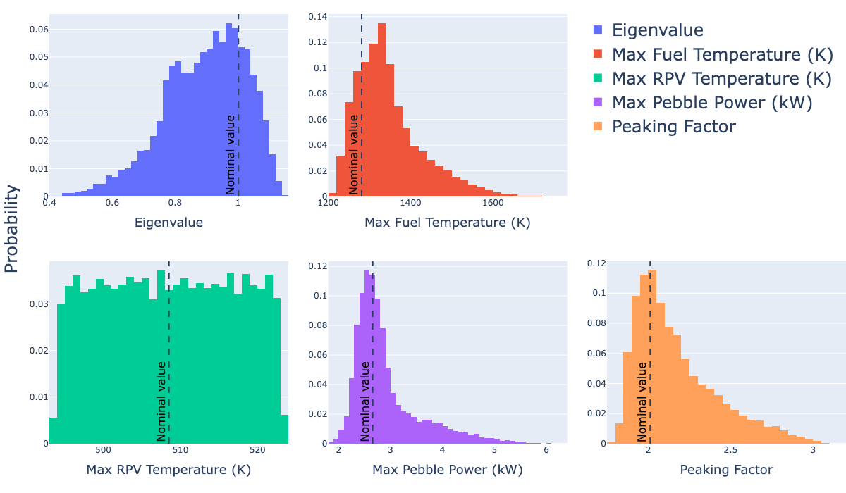
Figure 2: Discrete probability density functions of quantities of interest from Latin hypercube sampling.
Global Sensitivity Analysis
The final aspect of this demonstrative model is to use the data from previous section and evaluate Sobol indices using a polynomial chaos expansion (PCE) methodology. PCE is a surrogate modeling technique that has convenient feature for computing Sobol indices, for more details see Section 3.4 in Prince et al. (2024). The first part of this input involves loading the CSV data from the sampling run; the parameter data is loaded into a CSVSampler and the rest is loading into a CSVReaderVectorPostprocessor. Note that this data was processed with the following python commands to remove unconverged samples.
>>> import pandas as pd
>>> df = pd.read_csv("stm_lhs_sampling_out_storage_0001.csv")
>>> df = df.loc[df["data:converged"] == True]
>>> df.to_csv("stm_lhs_sampling_processed.csv", index=False)
[Samplers]
  [params]
    type = CSVSampler
    samples_file = stm_lhs_sampling_processed.csv
    column_names = 'kernel_radius
                    filling_factor
                    enrichment
                    pebble_unloading_rate
                    burnup_limit_weight
                    total_power'
  []
[]

[VectorPostprocessors]
  [qois]
    type = CSVReaderVectorPostprocessor
    csv_file = stm_lhs_sampling_processed.csv
  []
[]Next, Trainers are defined to train a fourth-order polynomial chaos expansion for each QoI using ordinary least-squares. Note the distributions from the sampling phase are required in order to select the optimal expansion bases.
[GlobalParams]
  sampler = params
  distributions = 'kr ff enrich pur bul power'
  order = 4
  regression_type = ols
[]

[Trainers]
  [train_eigenvalue]
    type = PolynomialChaosTrainer
    response = 'qois/data:eigenvalue:value'
    execute_on = timestep_begin
  []
  [train_pebble_power_max]
    type = PolynomialChaosTrainer
    response = 'qois/data:pebble_power_max:value'
    execute_on = timestep_begin
  []
  [train_peaking_factor]
    type = PolynomialChaosTrainer
    response = 'qois/data:peaking_factor:value'
    execute_on = timestep_begin
  []
  [train_Tfuel_max]
    type = PolynomialChaosTrainer
    response = 'qois/data:Tfuel_max:value'
    execute_on = timestep_begin
  []
  [train_Trpv_max]
    type = PolynomialChaosTrainer
    response = 'qois/data:Trpv_max:value'
    execute_on = timestep_begin
  []
[]Next, Surrogates for each QoI's PCE is specified.
[Surrogates]
  [model_eigenvalue]
    type = PolynomialChaos
    trainer = train_eigenvalue
  []
  [model_pebble_power_max]
    type = PolynomialChaos
    trainer = train_pebble_power_max
  []
  [model_peaking_factor]
    type = PolynomialChaos
    trainer = train_peaking_factor
  []
  [model_Tfuel_max]
    type = PolynomialChaos
    trainer = train_Tfuel_max
  []
  [model_Trpv_max]
    type = PolynomialChaos
    trainer = train_Trpv_max
  []
[]These Surrogates are used by a PolynomialChaosReporter to evaluate the first, second, and total Sobol indices.
[Reporters]
  [stats]
    type = PolynomialChaosReporter
    pc_name = 'model_eigenvalue
               model_pebble_power_max
               model_peaking_factor
               model_Tfuel_max
               model_Trpv_max'
    statistics = 'mean stddev'
    include_sobol = true
  []
[]Finally, the indices computed in the reporter are outputted via a JSON file.
[Outputs]
  json = true
  execute_on = timestep_end
[]This input can be run with any MOOSE executable that contains the STM, including moose-opt, griffin-opt, and blue_crab-opt. The run-time is essentially instantaneous on a single processor. Figure 3 shows the resulting total Sobol indices for each parameter-QoI pair.
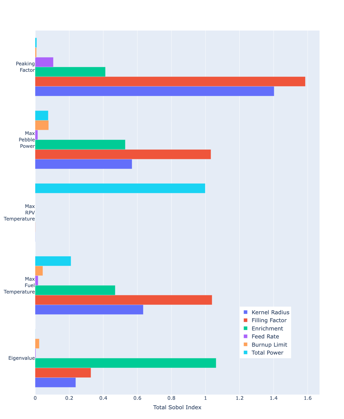
Figure 3: Total Sobol indices for each parameter and QoI calculated from polynomial chaos surrogate.
References
- Zachary M. Prince, Paolo Balestra, Javier Ortensi, Sebastian Schunert, Olin Calvin, Joshua T. Hanophy, Kun Mo, and Gerhard Strydom.
Sensitivity analysis, surrogate modeling, and optimization of pebble-bed reactors considering normal and accident conditions.
Nuclear Engineering and Design, 428:113466, 2024.
doi:https://doi.org/10.1016/j.nucengdes.2024.113466.[BibTeX]
@article{prince2024Sensitivity, author = "Prince, Zachary M. and Balestra, Paolo and Ortensi, Javier and Schunert, Sebastian and Calvin, Olin and Hanophy, Joshua T. and Mo, Kun and Strydom, Gerhard", title = "Sensitivity analysis, surrogate modeling, and optimization of pebble-bed reactors considering normal and accident conditions", journal = "Nuclear Engineering and Design", volume = "428", pages = "113466", year = "2024", issn = "0029-5493", doi = "https://doi.org/10.1016/j.nucengdes.2024.113466" } - Andrew E Slaughter, Zachary M Prince, Peter German, Ian Halvic, Wen Jiang, Benjamin W Spencer, Somayajulu L N Dhulipala, and Derek R Gaston.
MOOSE Stochastic Tools: A module for performing parallel, memory-efficient in situ stochastic simulations.
SoftwareX, 22:101345, 2023.
doi:10.1016/j.softx.2023.101345.[BibTeX]
@article{Slaughter2023,
    author = "Slaughter, Andrew E and Prince, Zachary M and German, Peter and Halvic, Ian and Jiang, Wen and Spencer, Benjamin W and Dhulipala, Somayajulu L N and Gaston, Derek R",
    doi = "10.1016/j.softx.2023.101345",
    issn = "2352-7110",
    journal = "SoftwareX",
    keywords = "MOOSE,Multiphysics,Parallel,Stochastic",
    pages = "101345",
    title = "{MOOSE Stochastic Tools: A module for performing parallel, memory-efficient in situ stochastic simulations}",
    volume = "22",
    year = "2023"
}
(htgr/gpbr200/sensitivity_analysis/stm_base_sampling.i)
# ==============================================================================
# Model description:
# Base stochastic tools sampling input for GPBR200 equilibrium core model.
# Cannot be run on its own without a sampler named "sample" defined.
# This sampler must have six columns representing:
#     1. TRISO kernel radius (m)
#     2. Particle filling factor
#     3. U235 enrichment in weight fraction
#     4. Pebble unloading rate (pebbles/second)
#     5. Burnup limit (MWd/kgHM)
#     6. Reactor thermal power (W)
# The output is a CSV file with the provided samples and five QoIs:
#     1. Eigenvalue
#     2. Max fuel temperature (K)
#     3. Max RPV temperature (K)
#     4. Max pebble power (W)
#     5. Peaking factor
# ------------------------------------------------------------------------------
# Idaho Falls, INL, May 29, 2025
# Author(s)(name alph): Dr. Zachary Prince
# ==============================================================================

# Kernel radius (m) ------------------------------------------------------------
kernel_radius_min = 1.5e-4
kernel_radius_max = 3.0e-4

# Filling factor ---------------------------------------------------------------
filling_factor_min = 0.05
filling_factor_max = 0.15

# Enrichment -------------------------------------------------------------------
enrichment_min = 0.05
enrichment_max = 0.2

# Pebble unloading rate (pebbles per second) -----------------------------------
pebble_unloading_rate_min = '${fparse 1.0/60}'
pebble_unloading_rate_max = '${fparse 3.0/60}'

# Burnup limit (MWD/kg) --------------------------------------------------------
burnup_limit_weight_min = 131.2 # MWd / kg
burnup_limit_weight_max = 164 # MWd / kg

# Total power (W) --------------------------------------------------------------
total_power_min = 180e6
total_power_max = 220e6

[StochasticTools]
[]

[MultiApps]
  [sub]
    type = SamplerFullSolveMultiApp
    input_files = gpbr200_ss_gfnk_reactor.i
    sampler = sample
    mode = batch-reset
    min_procs_per_app = 4
    ignore_solve_not_converge = true
  []
[]

[Controls]
  [param]
    type = MultiAppSamplerControl
    sampler = sample
    multi_app = sub
    param_names = 'kernel_radius
                   filling_factor
                   enrichment
                   pebble_unloading_rate
                   burnup_limit_weight
                   total_power'
  []
[]

[Reporters]
  [storage]
    type = StochasticMatrix
    sampler = sample
    sampler_column_names = 'kernel_radius
                            filling_factor
                            enrichment
                            pebble_unloading_rate
                            burnup_limit_weight
                            total_power'
    parallel_type = ROOT
  []
[]

[Transfers]
  [data]
    type = SamplerReporterTransfer
    from_multi_app = sub
    sampler = sample
    stochastic_reporter = storage
    from_reporter = 'eigenvalue/value
                     Tfuel_max/value
                     Trpv_max/value
                     pebble_power_max/value
                     peaking_factor/value'
  []
[]

[Outputs]
  csv = true
  execute_on = 'TIMESTEP_END'
[]
(htgr/gpbr200/sensitivity_analysis/stm_grid_study.i)
# ==============================================================================
# Model description:
# Grid study for select parameters and quantities of interest for GPBR200
# equilibrium core model.
# ------------------------------------------------------------------------------
# Idaho Falls, INL, May 29, 2025
# Author(s)(name alph): Dr. Zachary Prince
# ==============================================================================

!include stm_base_sampling.i

# Nominal parameter values -----------------------------------------------------
kernel_radius = 2.1250e-04
filling_factor = 0.0934404551647307 # Particle filling factor
enrichment = 0.155 # Enrichment in weight fraction
pebble_unloading_rate = '${fparse 1.5/60}' # pebbles per minute / seconds per minute.
burnup_limit_weight = 147.6 # MWd / kg
total_power = 200.0e+6 # Total reactor Power (W)

# Grid stepping ----------------------------------------------------------------
ngrid = 12
kernel_radius_step = '${fparse (kernel_radius_max - kernel_radius_min) / (ngrid - 1)}'
filling_factor_step = '${fparse (filling_factor_max - filling_factor_min) / (ngrid - 1)}'
enrichment_step = '${fparse (enrichment_max - enrichment_min) / (ngrid - 1)}'
pebble_unloading_rate_step = '${fparse (pebble_unloading_rate_max - pebble_unloading_rate_min) / (ngrid - 1)}'
burnup_limit_weight_step = '${fparse (burnup_limit_weight_max - burnup_limit_weight_min) / (ngrid - 1)}'
total_power_step = '${fparse (total_power_max - total_power_min) / (ngrid - 1)}'

[Samplers]
  [sample]
    type = Cartesian1D
    nominal_values = '${kernel_radius} ${filling_factor} ${enrichment} ${pebble_unloading_rate} ${burnup_limit_weight} ${total_power}'
    linear_space_items = '${kernel_radius_min} ${kernel_radius_step} ${ngrid}
                          ${filling_factor_min} ${filling_factor_step} ${ngrid}
                          ${enrichment_min} ${enrichment_step} ${ngrid}
                          ${pebble_unloading_rate_min} ${pebble_unloading_rate_step} ${ngrid}
                          ${burnup_limit_weight_min} ${burnup_limit_weight_step} ${ngrid}
                          ${total_power_min} ${total_power_step} ${ngrid}'
    min_procs_per_row = 4
    execute_on = PRE_MULTIAPP_SETUP
  []
[]
(htgr/gpbr200/sensitivity_analysis/stm_lhs_sampling.i)
# ==============================================================================
# Model description:
# Latin hypercube sampling for select parameters and quantities of interest for
# GPBR200 equilibrium core model.
# ------------------------------------------------------------------------------
# Idaho Falls, INL, May 29, 2025
# Author(s)(name alph): Dr. Zachary Prince
# ==============================================================================

!include stm_base_sampling.i

[Distributions]
  [kr]
    type = Uniform
    lower_bound = ${kernel_radius_min}
    upper_bound = ${kernel_radius_max}
  []
  [ff]
    type = Uniform
    lower_bound = ${filling_factor_min}
    upper_bound = ${filling_factor_max}
  []
  [enrich]
    type = Uniform
    lower_bound = ${enrichment_min}
    upper_bound = ${enrichment_max}
  []
  [pur]
    type = Uniform
    lower_bound = ${pebble_unloading_rate_min}
    upper_bound = ${pebble_unloading_rate_max}
  []
  [bul]
    type = Uniform
    lower_bound = ${burnup_limit_weight_min}
    upper_bound = ${burnup_limit_weight_max}
  []
  [power]
    type = Uniform
    lower_bound = ${total_power_min}
    upper_bound = ${total_power_max}
  []
[]

[Samplers]
  [sample]
    type = LatinHypercube
    distributions = 'kr ff enrich pur bul power'
    num_rows = 10000
    min_procs_per_row = 4
    execute_on = PRE_MULTIAPP_SETUP
  []
[]
(htgr/gpbr200/sensitivity_analysis/stm_poly_chaos.i)
# ==============================================================================
# Model description:
# This input takes the results from running stm_lhs_sampling.i and performs
# global sensitivity analysis using polynomial chaos methodology. The result is
# a JSON file containing the mean and standard deviation of the quantities of
# interest, as well as first, total, and second order Sobol indices w.r.t. every
# sampled parameter.
# ------------------------------------------------------------------------------
# Idaho Falls, INL, June 9, 2025
# Author(s)(name alph): Dr. Zachary Prince
# ==============================================================================

# Kernel radius (m) ------------------------------------------------------------
kernel_radius_min = 1.5e-4
kernel_radius_max = 3.0e-4

# Filling factor ---------------------------------------------------------------
filling_factor_min = 0.05
filling_factor_max = 0.15

# Enrichment -------------------------------------------------------------------
enrichment_min = 0.05
enrichment_max = 0.2

# Pebble unloading rate (pebbles per second) -----------------------------------
pebble_unloading_rate_min = '${fparse 1.0/60}'
pebble_unloading_rate_max = '${fparse 3.0/60}'

# Burnup limit (MWD/kg) --------------------------------------------------------
burnup_limit_weight_min = 131.2 # MWd / kg
burnup_limit_weight_max = 164 # MWd / kg

# Total power (W) --------------------------------------------------------------
total_power_min = 180e6
total_power_max = 220e6

[StochasticTools]
[]

[Distributions]
  [kr]
    type = Uniform
    lower_bound = ${kernel_radius_min}
    upper_bound = ${kernel_radius_max}
  []
  [ff]
    type = Uniform
    lower_bound = ${filling_factor_min}
    upper_bound = ${filling_factor_max}
  []
  [enrich]
    type = Uniform
    lower_bound = ${enrichment_min}
    upper_bound = ${enrichment_max}
  []
  [pur]
    type = Uniform
    lower_bound = ${pebble_unloading_rate_min}
    upper_bound = ${pebble_unloading_rate_max}
  []
  [bul]
    type = Uniform
    lower_bound = ${burnup_limit_weight_min}
    upper_bound = ${burnup_limit_weight_max}
  []
  [power]
    type = Uniform
    lower_bound = ${total_power_min}
    upper_bound = ${total_power_max}
  []
[]

[Samplers]
  [params]
    type = CSVSampler
    samples_file = stm_lhs_sampling_processed.csv
    column_names = 'kernel_radius
                    filling_factor
                    enrichment
                    pebble_unloading_rate
                    burnup_limit_weight
                    total_power'
  []
[]

[VectorPostprocessors]
  [qois]
    type = CSVReaderVectorPostprocessor
    csv_file = stm_lhs_sampling_processed.csv
  []
[]

[GlobalParams]
  sampler = params
  distributions = 'kr ff enrich pur bul power'
  order = 4
  regression_type = ols
[]

[Trainers]
  [train_eigenvalue]
    type = PolynomialChaosTrainer
    response = 'qois/data:eigenvalue:value'
    execute_on = timestep_begin
  []
  [train_pebble_power_max]
    type = PolynomialChaosTrainer
    response = 'qois/data:pebble_power_max:value'
    execute_on = timestep_begin
  []
  [train_peaking_factor]
    type = PolynomialChaosTrainer
    response = 'qois/data:peaking_factor:value'
    execute_on = timestep_begin
  []
  [train_Tfuel_max]
    type = PolynomialChaosTrainer
    response = 'qois/data:Tfuel_max:value'
    execute_on = timestep_begin
  []
  [train_Trpv_max]
    type = PolynomialChaosTrainer
    response = 'qois/data:Trpv_max:value'
    execute_on = timestep_begin
  []
[]

[Surrogates]
  [model_eigenvalue]
    type = PolynomialChaos
    trainer = train_eigenvalue
  []
  [model_pebble_power_max]
    type = PolynomialChaos
    trainer = train_pebble_power_max
  []
  [model_peaking_factor]
    type = PolynomialChaos
    trainer = train_peaking_factor
  []
  [model_Tfuel_max]
    type = PolynomialChaos
    trainer = train_Tfuel_max
  []
  [model_Trpv_max]
    type = PolynomialChaos
    trainer = train_Trpv_max
  []
[]

[Reporters]
  [stats]
    type = PolynomialChaosReporter
    pc_name = 'model_eigenvalue
               model_pebble_power_max
               model_peaking_factor
               model_Tfuel_max
               model_Trpv_max'
    statistics = 'mean stddev'
    include_sobol = true
  []
[]

[Outputs]
  json = true
  execute_on = timestep_end
[]
(htgr/gpbr200/sensitivity_analysis/gpbr200_ss_gfnk_reactor.i)
# ==============================================================================
# Model description:
# Equilibrium core neutronics model coupled with TH and pebble temperature
# models.
# ------------------------------------------------------------------------------
# Idaho Falls, INL, April 4, 2022 11:03 AM
# Author(s)(name alph): David Reger, Dr. Javier Ortensi, Dr. Paolo Balestra,
#   Dr. Ryan Stewart, Dr. Sebastian Schunert, Dr. Zachary Prince.
# ==============================================================================
# MODEL PARAMETERS
# ==============================================================================

# Power ------------------------------------------------------------------------
total_power = 200.0e+6 # Total reactor Power (W)

# Initial values ---------------------------------------------------------------
initial_temperature = 900.0 # (K)

# Geometry ---------------------------------------------------------------------
pbed_porosity = 0.39
pbed_top = 11.3354 # Absolute height of the core top in the model (m).

# Pebble Geometry --------------------------------------------------------------
pebble_radius = 3.0e-2 # pebble radius (m)
pebble_shell_thickness = 5.0e-03 # pebble fuel free zone thickness (graphite shell) (m)
pebble_volume = '${fparse 4/3*pi*pebble_radius^3}' # volume of the pebble (m3)
pebble_core_volume = '${fparse 4/3*pi*(pebble_radius-pebble_shell_thickness)^3}' # volume of the pebble occupied by TRISO (m3)
kernel_radius = 2.1250e-04 # kernel particle radius (m)
kernel_volume = '${fparse 4/3*pi*kernel_radius^3}' # volume of the kernel (m3)
buffer_thickness = 1.00e-04 # Thickness of buffer (m)
buffer_radius = '${fparse kernel_radius + buffer_thickness}' # Outer radius of buffer (m)
ipyc_thickness = 4.00e-05 # Thickness of IPyC (m)
ipyc_radius = '${fparse buffer_radius + ipyc_thickness}' # Outer radius of IPyC (m)
sic_thickness = 3.50e-05 # Thickness of SiC (m)
sic_radius = '${fparse ipyc_radius + sic_thickness}' # Outer radius of SiC (m)
opyc_thickness = 4.00e-05 # Thickness of OPyC (m)
opyc_radius = '${fparse sic_radius + opyc_thickness}' # Outer radius of OPyC (m)
triso_volume = '${fparse 4/3*pi*opyc_radius^3}' # volume of the particle (m3)
filling_factor = 0.0934404551647307 # Particle filling factor
triso_number = '${fparse pebble_core_volume * filling_factor / triso_volume}' # number of TRISO particle in a pebble (//)

# Compositions -----------------------------------------------------------------
enrichment = 0.155 # Enrichment in weight fraction
rho_kernel_UCO = 10.4 # Density of UCO (g/cm3)
ACU = 0.3920 # Carbon to Uranium atom ratio in UCO
AOU = 1.4280 # Oxygen to Uranium atom ratio in UCO

MU235 = 235.043929918 # Molar density of U235 (g/mol)
MU238 = 238.050788247 # Molar density of U238 (g/mol)
MC = 12.010735897 # Molar density of Carbon (g/mol)
MO = 15.994914620 # Molar density of Oxygen (g/mol)
enrichment_n = '${fparse enrichment/MU235 / (enrichment/MU235 + (1-enrichment)/MU238)}' # Enrichment in nuclide fration
MUCO = '${fparse MU235*enrichment_n + MU238*(1-enrichment_n) + MC*ACU + MO*AOU}' # UCO molar density (g/mol)
rhon_kernel_UCO = '${fparse rho_kernel_UCO / MUCO * 0.6022140}' # Molar density of UCO (atom/b/cm)

# Kernel number densities (n/b/cm)
rhon_kernel_U235 = '${fparse rhon_kernel_UCO * enrichment_n}'
rhon_kernel_U238 = '${fparse rhon_kernel_UCO * (1 - enrichment_n)}'
rhon_kernel_C = '${fparse rhon_kernel_UCO * ACU}'
rhon_kernel_O = '${fparse rhon_kernel_UCO * AOU}'

# Fractions of pebble volume
kernel_fraction = '${fparse kernel_volume * triso_number / pebble_volume}'

# Pebble volume densities (atoms/b/cm)
rhon_U235 = '${fparse rhon_kernel_U235 * kernel_fraction}'
rhon_U238 = '${fparse rhon_kernel_U238 * kernel_fraction}'

# Parameters describing pebble cycling -----------------------------------------
pebble_unloading_rate = '${fparse 1.5/60}' # pebbles per minute / seconds per minute.
burnup_limit_weight = 147.6 # MWd / kg
rho_U = '${fparse (rhon_U235*MU235 + rhon_U238*MU238) * 1.660539}' # Density of uranium in pebble volume (g/cm3)
burnup_conversion = '${fparse 1e9*3600*24*rho_U}' # Conversion from MWd/kg -> J/m3

# Blocks -----------------------------------------------------------------------
fuel_blocks = '5 6 7 8 9'
cns_disch_blocks = '14'
upref_blocks = '3 16'
upcav_blocks = '4'
lowref_blocks = '10 11 12 13'
crs_blocks = '17 22'
rdref_blocks = '1 2 15'
rpv_blocks = '18 19 20 21'
ref_blocks = '${cns_disch_blocks} ${upref_blocks}
              ${lowref_blocks}
              ${rdref_blocks}'

# ==============================================================================
# GLOBAL PARAMETERS
# ==============================================================================
[GlobalParams]
  is_meter = true
[]

# ==============================================================================
# GEOMETRY AND MESH
# ==============================================================================
[Mesh]
  [pebble_bed]
    type = FileMeshGenerator
    file = ../data/streamline_mesh_in.e
    exodus_extra_element_integers = 'pebble_streamline_id pebble_streamline_layer_id material_id'
  []
  coord_type = RZ
  rz_coord_axis = Y
[]

# ==============================================================================
# AUXVARIABLES AND AUXKERNELS
# ==============================================================================
[AuxVariables]
  # Temperatures.
  [T_solid]
    family = MONOMIAL
    order = CONSTANT
    initial_condition = ${initial_temperature}
    block = '${fuel_blocks} ${ref_blocks} ${crs_blocks} ${rpv_blocks}' # Everything but upper cavity
  []

  # Porosity
  [porosity]
    family = MONOMIAL
    order = CONSTANT
    block = '${fuel_blocks}'
    initial_condition = ${pbed_porosity}
  []
[]

# ==============================================================================
# MATERIALS
# ==============================================================================
[Materials]
  [reflector]
    type = CoupledFeedbackNeutronicsMaterial
    library_file = '../data/gpbr200_microxs.xml'
    library_name = 'gpbr200_microxs'
    grid_names = 'tmod'
    grid_variables = 'T_solid'
    isotopes = 'Graphite'
    densities = '8.82418e-2'
    plus = true
    material_id = 2
    diffusion_coefficient_scheme = local
    block = '${ref_blocks}'
  []
  [crs]
    type = CoupledFeedbackRoddedNeutronicsMaterial
    block = '${crs_blocks}'
    library_file = '../data/gpbr200_microxs.xml'
    library_name = 'gpbr200_microxs'
    grid_names = 'tmod'
    grid_variables = 'T_solid'

    isotopes = ' Graphite;
                 Graphite   B10        B11;
                 Graphite'
    densities = '8.82418e-2
                 7.1628E-02 8.9463E-03  2.2229E-03
                 8.82418e-2'

    rod_segment_length = 1e3
    front_position_function = 'cr_front'
    segment_material_ids = '2 2 2'
    rod_withdrawn_direction = 'y'
    average_segment_id = segment_id
  []
  [cavity]
    type = ConstantNeutronicsMaterial
    block = '${upcav_blocks}'
    fromFile = true
    library_file = '../data/gpbr200_void.xml'
    material_id = 10
  []
[]

[Functions]
  # Function describing CR depth
  [cr_depth]
    type = ConstantFunction
    value = 1.747 # Range of control rod insertion: -1.318 -> 8.93
  []
  # Offset from reactor reference frame
  [cr_front]
    type = ParsedFunction
    expression = 'top - cr_depth'
    symbol_names = 'top cr_depth'
    symbol_values = '${pbed_top} cr_depth'
  []
[]

[Compositions]
  [uco]
    type = IsotopeComposition
    density_type = atomic
    isotope_densities = '
      U235 ${rhon_kernel_U235}
      U238 ${rhon_kernel_U238}
      C12 ${rhon_kernel_C}
      O16 ${rhon_kernel_O}
    '
  []
  [buffer]
    type = IsotopeComposition
    density_type = atomic
    isotope_densities = 'Graphite 5.26466317651E-02'
  []
  [PyC]
    type = IsotopeComposition
    density_type = atomic
    isotope_densities = 'Graphite 9.52653336702E-02'
  []
  [SiC]
    type = IsotopeComposition
    density_type = atomic
    isotope_densities = '
      SI28 4.43270697709E-02
      SI29 2.25082086520E-03
      SI30 1.48375772443E-03
      C12  4.80616002990E-02
    '
  []
  [matrix]
    type = IsotopeComposition
    density_type = atomic
    isotope_densities = 'Graphite 8.67415932892E-02'
  []
  [triso]
    type = Triso
    compositions = 'uco buffer PyC SiC PyC'
    radii = '${kernel_radius} ${buffer_radius} ${ipyc_radius} ${sic_radius} ${opyc_radius}'
  []
  [triso_fill]
    type = StochasticComposition
    background_composition = matrix
    packing_fractions = ${filling_factor}
    triso_particles = triso
  []
  [pebble]
    type = Pebble
    compositions = 'triso_fill matrix'
    radii = '${fparse pebble_radius - pebble_shell_thickness} ${pebble_radius}'
  []
[]

# ==============================================================================
# PEBBLE DEPLETION
# ==============================================================================
[PebbleDepletion]
  block = '${fuel_blocks}'

  # Power.
  power = ${total_power}
  integrated_power_postprocessor = total_power
  power_density_variable = total_power_density
  family = MONOMIAL
  order = CONSTANT

  # Cross section data.
  library_file = '../data/gpbr200_microxs.xml'
  library_name = 'gpbr200_microxs'
  fuel_temperature_grid_name = 'tfuel'
  moderator_temperature_grid_name = 'tmod'
  burnup_grid_name = 'burnup'
  constant_grid_values = 'kernrad ${fparse kernel_radius * 1000}
                          fillfact ${filling_factor}
                          enrich ${enrichment}'

  # Transmutation data.
  dataset = ISOXML
  isoxml_data_file = '../data/gpbr200_dtl.xml'
  isoxml_lib_name = 'gpbr200_dtl'
  # Some of the branching ratios in the DTL are unphysical, which Griffin will
  # throw a warning for unless this is specified.
  dtl_physicality = 'SILENT'

  # Isotopic options
  n_fresh_pebble_types = 1
  fresh_pebble_compositions = 'pebble'

  # Pebble options
  porosity_name = porosity
  maximum_burnup = '${fparse 196.8 * burnup_conversion}'
  num_burnup_bins = 12

  # Tabulation data.
  initial_moderator_temperature = '${initial_temperature}'
  initial_fuel_temperature = '${initial_temperature}'

  [DepletionScheme]
    type = ConstantStreamlineEquilibrium

    # Streamline definition
    major_streamline_axis = y

    # Pebble options
    pebble_unloading_rate = ${pebble_unloading_rate}
    pebble_flow_rate_distribution = '0.12919675255653704 0.3237409742330389 0.16364127845178317 0.1970045449547337 0.1864164498039072'
    pebble_diameter = '${fparse pebble_radius * 2.0}'
    burnup_limit = '${fparse burnup_limit_weight * burnup_conversion}'

    # Solver parameters
    sweep_tol = 1e-8
    sweep_max_iterations = 20

    # Output
    exodus_streamline_output = false
  []

  diffusion_coefficient_scheme = local
[]

# ==============================================================================
# EXECUTION PARAMETERS
# ==============================================================================
[TransportSystems]
  particle = neutron
  equation_type = eigenvalue
  G = 9
  ReflectingBoundary = 'rinner'
  VacuumBoundary = 'rtop rbottom router'
  [diff]
    scheme = CFEM-Diffusion
    family = LAGRANGE
    order = FIRST
    n_delay_groups = 6
    assemble_scattering_jacobian = true
    assemble_fission_jacobian = true
    block = '${fuel_blocks} ${upcav_blocks} ${ref_blocks} ${crs_blocks}' # Excluding RPV and Barrel
  []
[]

[Executioner]
  type = Eigenvalue
  solve_type = 'PJFNKMO'
  constant_matrices = true
  petsc_options_iname = '-pc_type -pc_hypre_type -ksp_gmres_restart '
  petsc_options_value = 'hypre boomeramg 100'
  line_search = none

  # Linear/nonlinear iterations.
  l_max_its = 100
  l_tol = 1e-3

  nl_max_its = 50
  nl_rel_tol = 1e-7
  nl_abs_tol = 1e-9

  # Fixed point iterations.
  fixed_point_min_its = 15
  fixed_point_max_its = 200
  custom_pp = eigenvalue
  custom_abs_tol = 5e-5
  custom_rel_tol = 1e-50
  disable_fixed_point_residual_norm_check = true

  # Power iterations.
  free_power_iterations = 4
  extra_power_iterations = 20
[]

# ==============================================================================
# MULTIAPPS AND TRANSFERS
# ==============================================================================
[MultiApps]
  # Reactor TH.
  [pronghorn_th]
    type = FullSolveMultiApp
    input_files = gpbr200_ss_phth_reactor.i
    keep_solution_during_restore = true
    execute_on = 'TIMESTEP_END'
  []
[]

[Transfers]
  # TO Pronghorn.
  [to_pronghorn_total_power_density]
    type = MultiAppCopyTransfer
    to_multi_app = pronghorn_th
    source_variable = total_power_density
    variable = power_density
  []

  # FROM Pronghorn.
  [from_pronghorn_Tsolid]
    type = MultiAppCopyTransfer
    from_multi_app = pronghorn_th
    source_variable = T_solid
    variable = T_solid
  []
[]

# ==============================================================================
# Surrogates
# ==============================================================================
# Replace multiapps with surrogate model

[Surrogates]
  [Tfuel_model]
    type = PolynomialRegressionSurrogate
    filename = ../pebble_surrogate_modeling/stm_pebble_surrogate_model_pr6_Tfuel_train.rd
  []
  [Tmod_model]
    type = PolynomialRegressionSurrogate
    filename = ../pebble_surrogate_modeling/stm_pebble_surrogate_model_pr6_Tmod_train.rd
  []
[]

[AuxKernels]
  [Tfuel_aux]
    type = SurrogateModelArrayAuxKernel
    variable = triso_temperature
    model = Tfuel_model
    parameters = '${kernel_radius} ${filling_factor} T_solid partial_power_density'
    coupled_variables = T_solid
    coupled_array_variables = partial_power_density
    execute_on = TIMESTEP_BEGIN
  []
  [Tmod_aux]
    type = SurrogateModelArrayAuxKernel
    variable = graphite_temperature
    model = Tmod_model
    parameters = '${kernel_radius} ${filling_factor} T_solid partial_power_density'
    coupled_variables = T_solid
    coupled_array_variables = partial_power_density
    execute_on = TIMESTEP_BEGIN
  []
[]

# ==============================================================================
# POSTPROCESSING AND OUTPUTS
# ==============================================================================

[AuxVariables]
  # Max temperatures and power
  [Tfuel_max]
    family = MONOMIAL
    order = CONSTANT
    block = '${fuel_blocks}'
  []
  [Tmod_max]
    family = MONOMIAL
    order = CONSTANT
    block = '${fuel_blocks}'
  []
  [ppd_max]
    family = MONOMIAL
    order = CONSTANT
    block = '${fuel_blocks}'
  []
[]

[AuxKernels]
  # Max temperatures and power
  [Tfuel_max_aux]
    type = ArrayVarReductionAux
    variable = Tfuel_max
    array_variable = triso_temperature
    value_type = max
    execute_on = TIMESTEP_END
  []
  [Tmod_max_aux]
    type = ArrayVarReductionAux
    variable = Tmod_max
    array_variable = graphite_temperature
    value_type = max
    execute_on = TIMESTEP_END
  []
  [ppd_max_aux]
    type = ArrayVarReductionAux
    variable = ppd_max
    array_variable = partial_power_density
    value_type = max
    execute_on = TIMESTEP_END
  []
[]

[Postprocessors]
  # Temperatures
  [Tfuel_max]
    type = ElementExtremeValue
    variable = Tfuel_max
    block = ${fuel_blocks}
  []
  [Trpv_max]
    type = ElementExtremeValue
    variable = T_solid
    block = 21
  []

  # Pebble power
  [ppd_max]
    type = ElementExtremeValue
    variable = ppd_max
    block = ${fuel_blocks}
    outputs = none
  []
  [pebble_power_max]
    type = ScalePostprocessor
    value = ppd_max
    scaling_factor = '${pebble_volume}'
  []

  # Reactor power
  [power_max]
    type = ElementExtremeValue
    variable = total_power_density
    block = ${fuel_blocks}
    outputs = none
  []
  [power_avg]
    type = ElementAverageValue
    variable = total_power_density
    block = ${fuel_blocks}
    outputs = none
  []
  [peaking_factor]
    type = ParsedPostprocessor
    expression = 'power_max / power_avg'
    pp_names = 'power_max power_avg'
  []
[]
(htgr/gpbr200/pebble_surrogate_modeling/gpbr200_ss_phth_reactor.i)
# ==============================================================================
# Model description:
# gPBR200 thermal hydraulic model
# ------------------------------------------------------------------------------
# Idaho Falls, INL, Mar. 2023
# Author(s)(name alph): David Reger, Dr. Javier Ortensi, Dr. Paolo Balestra,
#   Dr. Ryan Stewart, Dr. Sebastian Schunert., Dr. Zachary M. Prince
# ==============================================================================
# MODEL PARAMETERS
# ==============================================================================

# Blocks -----------------------------------------------------------------------
risers_blocks = '1 2 3 22'
fluid_only_blocks = '4'
heated_blocks = '5 6 7 8 9'
outchans_blocks = '10'
outplen_blocks = '11'
hotleg_blocks = '12'
ref_blocks = '13 14 15 16 17'
ref2barrel_gap = '18'
barrel_blocks = '19'
barrel2rpv_gap = '20'
rpv_blocks = '21'
outlet_blocks = '${outplen_blocks} ${hotleg_blocks} ${outchans_blocks}'
porous_blocks = '${risers_blocks} ${heated_blocks} ${outlet_blocks}'
fluid_blocks = '${fluid_only_blocks} ${porous_blocks}'
solid_only_blocks = '${ref_blocks} ${barrel_blocks} ${rpv_blocks}'
pbed_blocks = '${heated_blocks}'
no_pbed_porous_blocks = '${risers_blocks} ${outlet_blocks}'

# Geometry ---------------------------------------------------------------------
pbed_r = 1.200 # Pebble Bed radius (m).
pbed_top = 11.3354 # Absolute height of the core top in the model (m).
rpv_r = 2.307 # rpv radius (m)
cavity_thickness = 1.340 # Cavity thickness from pbmr400 (m)
pebble_diameter = 0.06 # Diameter of the pebbles (m).

# Properties -------------------------------------------------------------------
global_emissivity = 0.80 # All the materials have the same emissivity (//).
reactor_total_mfr = 64.3 # Total reactor He mass flow rate (kg/s).
reactor_inlet_T_fluid = 533.25 # He temperature  at the inlet of the lower inlet plenum (K).
reactor_inlet_rho = 5.364 # He density at the inlet of the lower inlet plenum (kg/m3).
reactor_outlet_pressure = 5.84e+6 # Pressure at the at the outlet of the outlet plenum (Pa).
top_bottom_cav_temperature = '${fparse 273.15 + 200.0}' # Top and Bottom cavities temperatures (K).
rccs_temperature = '${fparse 273.15 + 70.0}' # RCCS temperatures (K).
htc_cavities = 10.0 # Heat Exchange coefficient for natural circulation (W/m2K)
heat_capacity_multiplier = 1e-5
db_cnst = 0.023 # Dittus Boelter constant for area htc
pbed_porosity = 0.39 # Pebble bed porosity (//).

# BCs --------------------------------------------------------------------------
inlet_free_area = '${fparse 2 * pi * 2.066 * 0.39}'
inlet_vel = '${fparse reactor_total_mfr/inlet_free_area/reactor_inlet_rho}'

# Initial values ---------------------------------------------------------------
pbed_free_flow_area = '${fparse pi * pbed_r * pbed_r}' # Core inlet free flow area (m2)
pbed_superficial_vel = '${fparse -reactor_total_mfr/pbed_free_flow_area/reactor_inlet_rho}' # m/s
initial_temp = 900.0 # K

[GlobalParams]
  pebble_diameter = ${pebble_diameter}
  acceleration = ' 0.00 -9.81 0.00 ' # Gravity acceleration (m/s2).
  fp = fluid_properties_obj
[]

# ==============================================================================
# GEOMETRY AND MESH
# ==============================================================================
[Mesh]
  [pebble_bed]
    type = FileMeshGenerator
    file = ../data/streamline_mesh_in.e
  []
  coord_type = RZ
  rz_coord_axis = Y
[]

[Problem]
  kernel_coverage_check = false
  material_coverage_check = false
[]

# ==============================================================================
# PHYSICS
# ==============================================================================
[Physics]
  [NavierStokes]
    [Flow]
      [flow]
        # Basic FVM settings
        block = '${fluid_blocks}'
        compressibility = 'weakly-compressible'
        gravity = '0.0 -9.81 0.0'

        # Porous treatment.
        porous_medium_treatment = true
        friction_types = 'darcy forchheimer'
        friction_coeffs = 'Darcy_coefficient Forchheimer_coefficient'
        porosity_interface_pressure_treatment = 'bernoulli'

        # Fluid properties.
        density = 'rho'
        dynamic_viscosity = 'mu'

        # Initial conditions.
        initial_velocity = '0 pbed_superficial_vel_func 0'
        velocity_variable = 'superficial_vel_x superficial_vel_y'
        initial_pressure = '${reactor_outlet_pressure}'

        # Fluid boundary conditions.
        inlet_boundaries = 'inlet'
        momentum_inlet_types = 'fixed-velocity'
        momentum_inlet_functors = '-${inlet_vel} 0'

        outlet_boundaries = 'outlet'
        momentum_outlet_types = 'fixed-pressure'
        pressure_functors = '${reactor_outlet_pressure}'

        wall_boundaries = 'wall inner'
        momentum_wall_types = 'slip  symmetry'
      []
    []
    [FluidHeatTransfer]
      [energy]
        block = '${fluid_blocks}'

        # Fluid properties.
        thermal_conductivity = 'kappa'
        specific_heat = 'cp'

        # Initial conditions
        fluid_temperature_variable = 'T_fluid'
        initial_temperature = '${initial_temp}'

        # Fluid boundary conditions
        energy_inlet_types = 'fixed-temperature'
        energy_inlet_functors = '${reactor_inlet_T_fluid}'
        energy_wall_types = 'heatflux  heatflux'
        energy_wall_functors = '0         0'

        # Convective heat transfer.
        ambient_convection_blocks = '${porous_blocks}'
        ambient_convection_alpha = 'alpha'
        ambient_temperature = 'T_solid'

        # Interpolation schemes.
        energy_advection_interpolation = average
      []
    []
    [SolidHeatTransfer]
      [solid]
        block = '${porous_blocks} ${solid_only_blocks} ${ref2barrel_gap} ${barrel2rpv_gap}'

        # Initial conditions.
        solid_temperature_variable = 'T_solid'
        initial_temperature = ${initial_temp}

        # Solid properties
        thermal_conductivity_solid = 'effective_thermal_conductivity'
        cp_solid = 'cp_s_mod'
        rho_solid = 'rho_s'

        # Convective heat transfer.
        ambient_convection_blocks = '${porous_blocks}'
        ambient_convection_alpha = 'alpha'
        ambient_convection_temperature = 'T_fluid'

        # Heat source
        external_heat_source_blocks = '${heated_blocks}'
        external_heat_source = 'power_density'
      []
    []
  []
[]

[FVBCs]
  [rpv_radial_radiation]
    type = FVInfiniteCylinderRadiativeBC
    variable = T_solid
    cylinder_emissivity = '${global_emissivity}'
    boundary_emissivity = '${global_emissivity}'
    boundary_radius = '${rpv_r}'
    cylinder_radius = '${fparse rpv_r + cavity_thickness}'
    Tinfinity = '${rccs_temperature}'
    boundary = 'rpv2rcav'
  []
  [rpv_radial_convection]
    type = FVFunctorConvectiveHeatFluxBC
    variable = T_solid
    T_solid = T_solid
    T_bulk = '${rccs_temperature}'
    boundary = 'rpv2rcav'
    heat_transfer_coefficient = '${htc_cavities}'
    is_solid = true
  []
  [rpv_bottom_top]
    type = FVFunctorConvectiveHeatFluxBC
    variable = T_solid
    T_solid = T_solid
    T_bulk = '${top_bottom_cav_temperature}'
    boundary = 'rtop rbottom'
    heat_transfer_coefficient = '${htc_cavities}'
    is_solid = true
  []
[]

# ==============================================================================
# AUXVARIABLES AND AUXKERNELS
# ==============================================================================
[AuxVariables]
  [power_density]
    family = MONOMIAL
    order = CONSTANT
    fv = true
    block = '${heated_blocks}'
  []

  [vel_x]
    family = MONOMIAL
    order = CONSTANT
    fv = true
    block = '${fluid_blocks}'
  []
  [vel_y]
    family = MONOMIAL
    order = CONSTANT
    fv = true
    block = '${fluid_blocks}'
  []
[]

[AuxKernels]
  [vel_x]
    type = InterstitialFunctorAux
    variable = vel_x
    superficial_variable = superficial_vel_x
    phase = fluid
    porosity = porosity
  []
  [vel_y]
    type = InterstitialFunctorAux
    variable = vel_y
    superficial_variable = superficial_vel_y
    phase = fluid
    porosity = porosity
  []
[]

# ==============================================================================
# INITIAL CONDITIONS AND FUNCTIONS
# ==============================================================================

[Functions]
  [pbed_superficial_vel_func]
    type = ParsedFunction
    expression = 'if(x < pbed_r & y > 1.851 & y < pbed_top, vel, 0.0)'
    symbol_names = 'pbed_r pbed_top vel'
    symbol_values = '${pbed_r} ${pbed_top} ${pbed_superficial_vel}'
  []
  [he_conductivity_fn]
    type = PiecewiseLinear
    x = '300 350 400 450 500 550 600 650 700 750 800 850 900 950
         1000 1050 1100 1150 1200 1250 1300 1350 1400 1450 1500'
    y = '1.57e-01 1.75e-01 1.92e-01
         2.08e-01 2.24e-01 2.40e-01 2.55e-01 2.69e-01 2.84e-01 2.98e-01 3.12e-01
         3.25e-01 3.38e-01 3.51e-01 3.64e-01 3.77e-01 3.89e-01 4.02e-01
         4.14e-01 4.26e-01 4.38e-01 4.50e-01 4.61e-01 4.73e-01 4.84e-01'
  []
[]

# ==============================================================================
# FLUID PROPERTIES, MATERIALS AND USER OBJECTS
# ==============================================================================
[FluidProperties]
  [fluid_properties_obj]
    type = HeliumFluidProperties
  []
[]

[FunctorMaterials]
  # Fluid properties and non-dimensional numbers.
  [fluid_props_to_mat_props]
    type = GeneralFunctorFluidProps
    pressure = 'pressure'
    T_fluid = 'T_fluid'
    speed = 'speed'
    porosity = porosity
    characteristic_length = characteristic_length
    block = ${fluid_blocks}
  []

  # Porosity.
  [risers_blocks_porosity]
    type = ADGenericFunctorMaterial
    prop_names = 'porosity'
    prop_values = '0.22' # 18 channels and inlet structures (//).
    block = '${risers_blocks}'
  []
  [pbed_blocks_porosity]
    type = ADGenericFunctorMaterial
    prop_names = 'porosity'
    prop_values = '${pbed_porosity}'
    block = ' ${heated_blocks}'
  []
  [cavity_blocks_porosity]
    type = ADGenericFunctorMaterial
    prop_names = 'porosity'
    prop_values = '0.99' # Ideally 1.0 (//).
    block = '${fluid_only_blocks}'
  []
  [outchans_blocks_porosity]
    type = ADGenericFunctorMaterial
    prop_names = 'porosity'
    prop_values = '0.63' # Triangular lattice of 0.5cm radius channels and 1.7cm pitch (//).
    block = '${outchans_blocks}'
  []
  [outplen_blocks_porosity]
    type = ADGenericFunctorMaterial
    prop_names = 'porosity'
    prop_values = '0.40' # Triangular lattice of 4.75cm radius colums and 16.5cm pitch (//).
    block = '${outplen_blocks}'
  []
  [hotleg_blocks_porosity]
    type = ADGenericFunctorMaterial
    prop_names = 'porosity'
    prop_values = '0.07' # Cylindrical channel (//).
    block = '${hotleg_blocks}'
  []
  [all_other_porosity]
    type = ADGenericFunctorMaterial
    prop_names = 'porosity'
    prop_values = '-1' # Dummy value.
    block = '${solid_only_blocks} ${ref2barrel_gap} ${barrel2rpv_gap}'
  []

  # Characteristic Length.
  [pbed_hydraulic_diameter]
    type = GenericFunctorMaterial
    prop_names = 'characteristic_length'
    prop_values = '${pebble_diameter}'
    block = '${pbed_blocks}'
  []
  [risers_hydraulic_diameter]
    type = GenericFunctorMaterial
    prop_names = 'characteristic_length'
    prop_values = '0.17' # Diameter of the risers channels (m).
    block = '${risers_blocks} ${fluid_only_blocks}'
  []
  [outlet_chans_hydraulic_diameter]
    type = GenericFunctorMaterial
    prop_names = 'characteristic_length'
    prop_values = '0.01' # Diameter of the outlet channels (m).
    block = '${outchans_blocks}'
  []
  [outlet_plen_hydraulic_diameter]
    type = GenericFunctorMaterial
    prop_names = 'characteristic_length'
    prop_values = '0.25' # Hydraulic diameter of outlet plenum (m).
    block = '${outplen_blocks}'
  []
  [hotleg_hydraulic_diameter]
    type = GenericFunctorMaterial
    prop_names = 'characteristic_length'
    prop_values = '0.967' # Diameter of the hot leg (m).
    block = '${hotleg_blocks}'
  []

  # Solid properties.
  [full_density_graphite]
    type = ADGenericFunctorMaterial
    prop_names = 'rho_s cp_s k_s'
    prop_values = '1780 1697 26'
    block = '${ref_blocks} ${risers_blocks} ${outlet_blocks} ${heated_blocks}'
  []
  [core_barrel_steel]
    type = ADGenericFunctorMaterial
    prop_names = 'rho_s cp_s k_s'
    prop_values = '7800.0 540.0 17.0'
    block = '${barrel_blocks}'
  []
  [rpv_steel]
    type = ADGenericFunctorMaterial
    prop_names = 'rho_s cp_s k_s'
    prop_values = '7800.0 525.0 38.0'
    block = '${rpv_blocks}'
  []
  [he_rho_and_cp]
    type = ADGenericFunctorMaterial
    prop_names = 'rho_s  cp_s'
    prop_values = '6      5000'
    block = '${ref2barrel_gap} ${barrel2rpv_gap}'
  []
  [mod_cp_s]
    type = ADParsedFunctorMaterial
    expression = 'cp_s * ${heat_capacity_multiplier}'
    property_name = 'cp_s_mod'
    functor_symbols = 'cp_s'
    functor_names = 'cp_s'
    block = '${porous_blocks} ${solid_only_blocks} ${ref2barrel_gap} ${barrel2rpv_gap}'
  []

  # Drag coefficients.
  [pbed_drag_coefficient]
    type = FunctorKTADragCoefficients
    T_fluid = T_fluid
    T_solid = T_solid
    porosity = porosity
    block = '${pbed_blocks}'
  []
  [risers_drag_coefficients]
    type = FunctorChurchillDragCoefficients
    block = '${risers_blocks} ${fluid_only_blocks}'
  []
  [outchans_drag_coefficients]
    type = FunctorChurchillDragCoefficients
    multipliers = '1.0e+05 1.0 1.0e+05'
    block = '${outchans_blocks}'
  []
  [outlet_drag_coefficients]
    type = FunctorChurchillDragCoefficients
    block = '${outplen_blocks}'
  []
  [hotleg_drag_coefficients]
    type = FunctorChurchillDragCoefficients
    multipliers = '1.0 1.0e+05 1.0e+05'
    block = '${hotleg_blocks}'
  []

  # Heat transfer coefficients.
  [pbed_alpha]
    type = FunctorKTAPebbleBedHTC
    T_solid = T_solid
    T_fluid = T_fluid
    mu = mu
    porosity = porosity
    pressure = pressure
    block = '${pbed_blocks}'
  []
  [risers_blocks_alpha]
    type = FunctorDittusBoelterWallHTC
    C = '${fparse db_cnst * 23.5}'

    block = '${risers_blocks}'
  []
  [outchans_blocks_alpha]
    type = FunctorDittusBoelterWallHTC
    C = '${fparse db_cnst * 400}'
    block = '${outchans_blocks}'
  []
  [outplen_blocks_alpha]
    type = FunctorDittusBoelterWallHTC
    C = '${fparse db_cnst * 63.5}'
    block = '${outplen_blocks}'
  []
  [rename_wall_htc_to_alpha]
    type = ADGenericFunctorMaterial
    prop_values = 'wall_htc'
    prop_names = 'alpha'
    block = '${risers_blocks} ${outchans_blocks} ${outplen_blocks}'
  []
  [hotleg_blocks_alpha]
    type = ADGenericFunctorMaterial
    prop_names = 'alpha'
    prop_values = '0.0'
    block = '${hotleg_blocks}'
  []

  # Effective solid thermal conductivity.
  [pebble_effective_thermal_conductivity]
    type = FunctorPebbleBedKappaSolid
    T_solid = T_solid
    porosity = porosity
    solid_conduction = ZBS
    emissivity = 0.8
    infinite_porosity = '${pbed_porosity}'
    Youngs_modulus = 9e+9
    Poisson_ratio = 0.1360
    lattice_parameters = interpolation
    coordination_number = You
    wall_distance = bed_geometry # Requested by solid_conduction = ZBS
    block = '${pbed_blocks}'
  []
  [porous_blocks_solid_effective_conductivity]
    type = FunctorVolumeAverageKappaSolid
    porosity = porosity
    block = '${no_pbed_porous_blocks}'
  []
  [effective_solid_thermal_conductivity]
    type = ADGenericVectorFunctorMaterial
    prop_names = 'effective_thermal_conductivity'
    prop_values = 'kappa_s kappa_s kappa_s'
    block = '${pbed_blocks} ${no_pbed_porous_blocks}'
  []
  [effective_solid_thermal_conductivity_solid_only]
    type = ADGenericVectorFunctorMaterial
    prop_names = 'effective_thermal_conductivity'
    prop_values = 'k_s k_s k_s'
    block = '${solid_only_blocks}'
  []
  [effective_thermal_conductivity_refl_ref2barrel_gap]
    type = FunctorGapHeatTransferEffectiveThermalConductivity
    gap_direction = x
    temperature = T_solid
    gap_conductivity_function = he_conductivity_fn
    emissivity_primary = ${global_emissivity}
    emissivity_secondary = ${global_emissivity}
    radius_primary = 2.066
    radius_secondary = 2.098
    prop_name = effective_thermal_conductivity
    block = '${ref2barrel_gap}'
  []
  [effective_thermal_conductivity_barrel_rpv_gap]
    type = FunctorGapHeatTransferEffectiveThermalConductivity
    gap_direction = x
    temperature = T_solid
    gap_conductivity_function = he_conductivity_fn
    emissivity_primary = ${global_emissivity}
    emissivity_secondary = ${global_emissivity}
    radius_primary = 2.143
    radius_secondary = 2.215
    prop_name = effective_thermal_conductivity
    block = '${barrel2rpv_gap}'
  []

  # Effective fluid thermal conductivity.
  [pebble_bed_effective_fluid_thermal_conductivity]
    type = FunctorLinearPecletKappaFluid
    porosity = porosity
    block = '${pbed_blocks}'
  []
  [everywhere_else_effective_fluid_thermal_conductivity]
    type = ADGenericVectorFunctorMaterial
    prop_names = 'kappa'
    prop_values = 'k k k'
    block = '${no_pbed_porous_blocks} ${fluid_only_blocks}'
  []
[]

[UserObjects]
  [bed_geometry]
    type = WallDistanceCylindricalBed
    top = '${pbed_top}'
    inner_radius = 0.0
    outer_radius = '${pbed_r}'
  []
[]

# ==============================================================================
# EXECUTION PARAMETERS
# ==============================================================================
[Executioner]
  type = Transient
  solve_type = NEWTON
  petsc_options_iname = '-pc_type'
  petsc_options_value = 'lu'
  line_search = l2

  # Scaling.
  automatic_scaling = true
  off_diagonals_in_auto_scaling = false
  compute_scaling_once = false

  # Tolerances.
  nl_abs_tol = 1e-5
  nl_rel_tol = 1e-6
  nl_max_its = 15

  # Time step control.
  [TimeStepper]
    type = IterationAdaptiveDT
    dt = 2.5e-3
    cutback_factor = 0.5
    growth_factor = 2.00
    optimal_iterations = 8
  []

  # Steady state detection.
  steady_state_detection = true
  steady_state_tolerance = 1e-13
[]

# ==============================================================================
# POSTPROCESSORS DEBUG AND OUTPUTS
# ==============================================================================
[Postprocessors]
  # General checks.
  [pp00_inlet_mfr]
    type = VolumetricFlowRate
    vel_x = 'superficial_vel_x'
    vel_y = 'superficial_vel_y'
    advected_quantity = rho
    boundary = inlet
    rhie_chow_user_object = pins_rhie_chow_interpolator
    execute_on = 'INITIAL TIMESTEP_END'
  []
  [pp01_outlet_mfr]
    type = VolumetricFlowRate
    vel_x = 'superficial_vel_x'
    vel_y = 'superficial_vel_y'
    advected_quantity = rho
    boundary = outlet
    rhie_chow_user_object = pins_rhie_chow_interpolator
    execute_on = 'INITIAL TIMESTEP_END'
  []
  [pp02_inlet_pressure]
    type = SideAverageValue
    variable = pressure
    boundary = 'inlet'
    execute_on = 'INITIAL TIMESTEP_END'
  []
  [pp03_total_power]
    type = ElementIntegralVariablePostprocessor
    variable = power_density
    block = '${heated_blocks}'
    execute_on = 'INITIAL TIMESTEP_END'
  []
  [pp04_T_oulet]
    type = SideAverageValue # Fix it with weighted thing
    variable = T_fluid
    boundary = 'outlet'
  []
  [pp05_rpv_temp]
    type = ElementAverageValue
    variable = T_solid
    block = '${rpv_blocks}'
  []
  [pp06_rpv_temp_max]
    type = ElementExtremeValue
    variable = T_solid
    block = '${rpv_blocks}'
  []
[]

[Outputs]
  exodus = true
  csv = true
  execute_on = 'FINAL'

  # Reduce console output
  print_linear_residuals = false
  print_linear_converged_reason = false
  print_nonlinear_converged_reason = false
[]
(htgr/gpbr200/sensitivity_analysis/gpbr200_ss_phth_reactor.i)
# ==============================================================================
# Model description:
# gPBR200 thermal hydraulic model
# ------------------------------------------------------------------------------
# Idaho Falls, INL, Mar. 2023
# Author(s)(name alph): David Reger, Dr. Javier Ortensi, Dr. Paolo Balestra,
#   Dr. Ryan Stewart, Dr. Sebastian Schunert., Dr. Zachary M. Prince
# ==============================================================================
# MODEL PARAMETERS
# ==============================================================================

# Blocks -----------------------------------------------------------------------
risers_blocks = '1 2 3 22'
fluid_only_blocks = '4'
heated_blocks = '5 6 7 8 9'
outchans_blocks = '10'
outplen_blocks = '11'
hotleg_blocks = '12'
ref_blocks = '13 14 15 16 17'
ref2barrel_gap = '18'
barrel_blocks = '19'
barrel2rpv_gap = '20'
rpv_blocks = '21'
outlet_blocks = '${outplen_blocks} ${hotleg_blocks} ${outchans_blocks}'
porous_blocks = '${risers_blocks} ${heated_blocks} ${outlet_blocks}'
fluid_blocks = '${fluid_only_blocks} ${porous_blocks}'
solid_only_blocks = '${ref_blocks} ${barrel_blocks} ${rpv_blocks}'
pbed_blocks = '${heated_blocks}'
no_pbed_porous_blocks = '${risers_blocks} ${outlet_blocks}'

# Geometry ---------------------------------------------------------------------
pbed_r = 1.200 # Pebble Bed radius (m).
pbed_top = 11.3354 # Absolute height of the core top in the model (m).
rpv_r = 2.307 # rpv radius (m)
cavity_thickness = 1.340 # Cavity thickness from pbmr400 (m)
pebble_diameter = 0.06 # Diameter of the pebbles (m).

# Properties -------------------------------------------------------------------
global_emissivity = 0.80 # All the materials have the same emissivity (//).
reactor_total_mfr = 64.3 # Total reactor He mass flow rate (kg/s).
reactor_inlet_T_fluid = 533.25 # He temperature  at the inlet of the lower inlet plenum (K).
reactor_inlet_rho = 5.364 # He density at the inlet of the lower inlet plenum (kg/m3).
reactor_outlet_pressure = 5.84e+6 # Pressure at the at the outlet of the outlet plenum (Pa).
top_bottom_cav_temperature = '${fparse 273.15 + 200.0}' # Top and Bottom cavities temperatures (K).
rccs_temperature = '${fparse 273.15 + 70.0}' # RCCS temperatures (K).
htc_cavities = 10.0 # Heat Exchange coefficient for natural circulation (W/m2K)
heat_capacity_multiplier = 1e-5
db_cnst = 0.023 # Dittus Boelter constant for area htc
pbed_porosity = 0.39 # Pebble bed porosity (//).

# BCs --------------------------------------------------------------------------
inlet_free_area = '${fparse 2 * pi * 2.066 * 0.39}'
inlet_vel = '${fparse reactor_total_mfr/inlet_free_area/reactor_inlet_rho}'

# Initial values ---------------------------------------------------------------
pbed_free_flow_area = '${fparse pi * pbed_r * pbed_r}' # Core inlet free flow area (m2)
pbed_superficial_vel = '${fparse -reactor_total_mfr/pbed_free_flow_area/reactor_inlet_rho}' # m/s
initial_temp = 900.0 # K

[GlobalParams]
  pebble_diameter = ${pebble_diameter}
  acceleration = ' 0.00 -9.81 0.00 ' # Gravity acceleration (m/s2).
  fp = fluid_properties_obj
[]

# ==============================================================================
# GEOMETRY AND MESH
# ==============================================================================
[Mesh]
  [pebble_bed]
    type = FileMeshGenerator
    file = ../data/streamline_mesh_in.e
  []
  coord_type = RZ
  rz_coord_axis = Y
[]

[Problem]
  kernel_coverage_check = false
  material_coverage_check = false
[]

# ==============================================================================
# PHYSICS
# ==============================================================================
[Physics]
  [NavierStokes]
    [Flow]
      [flow]
        # Basic FVM settings
        block = '${fluid_blocks}'
        compressibility = 'weakly-compressible'
        gravity = '0.0 -9.81 0.0'

        # Porous treatment.
        porous_medium_treatment = true
        friction_types = 'darcy forchheimer'
        friction_coeffs = 'Darcy_coefficient Forchheimer_coefficient'
        porosity_interface_pressure_treatment = 'bernoulli'

        # Fluid properties.
        density = 'rho'
        dynamic_viscosity = 'mu'

        # Initial conditions.
        initial_velocity = '0 pbed_superficial_vel_func 0'
        velocity_variable = 'superficial_vel_x superficial_vel_y'
        initial_pressure = '${reactor_outlet_pressure}'

        # Fluid boundary conditions.
        inlet_boundaries = 'inlet'
        momentum_inlet_types = 'fixed-velocity'
        momentum_inlet_functors = '-${inlet_vel} 0'

        outlet_boundaries = 'outlet'
        momentum_outlet_types = 'fixed-pressure'
        pressure_functors = '${reactor_outlet_pressure}'

        wall_boundaries = 'wall inner'
        momentum_wall_types = 'slip  symmetry'
      []
    []
    [FluidHeatTransfer]
      [energy]
        block = '${fluid_blocks}'

        # Fluid properties.
        thermal_conductivity = 'kappa'
        specific_heat = 'cp'

        # Initial conditions
        fluid_temperature_variable = 'T_fluid'
        initial_temperature = '${initial_temp}'

        # Fluid boundary conditions
        energy_inlet_types = 'fixed-temperature'
        energy_inlet_functors = '${reactor_inlet_T_fluid}'
        energy_wall_types = 'heatflux  heatflux'
        energy_wall_functors = '0         0'

        # Convective heat transfer.
        ambient_convection_blocks = '${porous_blocks}'
        ambient_convection_alpha = 'alpha'
        ambient_temperature = 'T_solid'

        # Interpolation schemes.
        energy_advection_interpolation = average
      []
    []
    [SolidHeatTransfer]
      [solid]
        block = '${porous_blocks} ${solid_only_blocks} ${ref2barrel_gap} ${barrel2rpv_gap}'

        # Initial conditions.
        solid_temperature_variable = 'T_solid'
        initial_temperature = ${initial_temp}

        # Solid properties
        thermal_conductivity_solid = 'effective_thermal_conductivity'
        cp_solid = 'cp_s_mod'
        rho_solid = 'rho_s'

        # Convective heat transfer.
        ambient_convection_blocks = '${porous_blocks}'
        ambient_convection_alpha = 'alpha'
        ambient_convection_temperature = 'T_fluid'

        # Heat source
        external_heat_source_blocks = '${heated_blocks}'
        external_heat_source = 'power_density'
      []
    []
  []
[]

[FVBCs]
  [rpv_radial_radiation]
    type = FVInfiniteCylinderRadiativeBC
    variable = T_solid
    cylinder_emissivity = '${global_emissivity}'
    boundary_emissivity = '${global_emissivity}'
    boundary_radius = '${rpv_r}'
    cylinder_radius = '${fparse rpv_r + cavity_thickness}'
    Tinfinity = '${rccs_temperature}'
    boundary = 'rpv2rcav'
  []
  [rpv_radial_convection]
    type = FVFunctorConvectiveHeatFluxBC
    variable = T_solid
    T_solid = T_solid
    T_bulk = '${rccs_temperature}'
    boundary = 'rpv2rcav'
    heat_transfer_coefficient = '${htc_cavities}'
    is_solid = true
  []
  [rpv_bottom_top]
    type = FVFunctorConvectiveHeatFluxBC
    variable = T_solid
    T_solid = T_solid
    T_bulk = '${top_bottom_cav_temperature}'
    boundary = 'rtop rbottom'
    heat_transfer_coefficient = '${htc_cavities}'
    is_solid = true
  []
[]

# ==============================================================================
# AUXVARIABLES AND AUXKERNELS
# ==============================================================================
[AuxVariables]
  [power_density]
    family = MONOMIAL
    order = CONSTANT
    fv = true
    block = '${heated_blocks}'
  []

  [vel_x]
    family = MONOMIAL
    order = CONSTANT
    fv = true
    block = '${fluid_blocks}'
  []
  [vel_y]
    family = MONOMIAL
    order = CONSTANT
    fv = true
    block = '${fluid_blocks}'
  []
[]

[AuxKernels]
  [vel_x]
    type = InterstitialFunctorAux
    variable = vel_x
    superficial_variable = superficial_vel_x
    phase = fluid
    porosity = porosity
  []
  [vel_y]
    type = InterstitialFunctorAux
    variable = vel_y
    superficial_variable = superficial_vel_y
    phase = fluid
    porosity = porosity
  []
[]

# ==============================================================================
# INITIAL CONDITIONS AND FUNCTIONS
# ==============================================================================

[Functions]
  [pbed_superficial_vel_func]
    type = ParsedFunction
    expression = 'if(x < pbed_r & y > 1.851 & y < pbed_top, vel, 0.0)'
    symbol_names = 'pbed_r pbed_top vel'
    symbol_values = '${pbed_r} ${pbed_top} ${pbed_superficial_vel}'
  []
  [he_conductivity_fn]
    type = PiecewiseLinear
    x = '300 350 400 450 500 550 600 650 700 750 800 850 900 950
         1000 1050 1100 1150 1200 1250 1300 1350 1400 1450 1500'
    y = '1.57e-01 1.75e-01 1.92e-01
         2.08e-01 2.24e-01 2.40e-01 2.55e-01 2.69e-01 2.84e-01 2.98e-01 3.12e-01
         3.25e-01 3.38e-01 3.51e-01 3.64e-01 3.77e-01 3.89e-01 4.02e-01
         4.14e-01 4.26e-01 4.38e-01 4.50e-01 4.61e-01 4.73e-01 4.84e-01'
  []
[]

# ==============================================================================
# FLUID PROPERTIES, MATERIALS AND USER OBJECTS
# ==============================================================================
[FluidProperties]
  [fluid_properties_obj]
    type = HeliumFluidProperties
  []
[]

[FunctorMaterials]
  # Fluid properties and non-dimensional numbers.
  [fluid_props_to_mat_props]
    type = GeneralFunctorFluidProps
    pressure = 'pressure'
    T_fluid = 'T_fluid'
    speed = 'speed'
    porosity = porosity
    characteristic_length = characteristic_length
    block = ${fluid_blocks}
  []

  # Porosity.
  [risers_blocks_porosity]
    type = ADGenericFunctorMaterial
    prop_names = 'porosity'
    prop_values = '0.22' # 18 channels and inlet structures (//).
    block = '${risers_blocks}'
  []
  [pbed_blocks_porosity]
    type = ADGenericFunctorMaterial
    prop_names = 'porosity'
    prop_values = '${pbed_porosity}'
    block = ' ${heated_blocks}'
  []
  [cavity_blocks_porosity]
    type = ADGenericFunctorMaterial
    prop_names = 'porosity'
    prop_values = '0.99' # Ideally 1.0 (//).
    block = '${fluid_only_blocks}'
  []
  [outchans_blocks_porosity]
    type = ADGenericFunctorMaterial
    prop_names = 'porosity'
    prop_values = '0.63' # Triangular lattice of 0.5cm radius channels and 1.7cm pitch (//).
    block = '${outchans_blocks}'
  []
  [outplen_blocks_porosity]
    type = ADGenericFunctorMaterial
    prop_names = 'porosity'
    prop_values = '0.40' # Triangular lattice of 4.75cm radius colums and 16.5cm pitch (//).
    block = '${outplen_blocks}'
  []
  [hotleg_blocks_porosity]
    type = ADGenericFunctorMaterial
    prop_names = 'porosity'
    prop_values = '0.07' # Cylindrical channel (//).
    block = '${hotleg_blocks}'
  []
  [all_other_porosity]
    type = ADGenericFunctorMaterial
    prop_names = 'porosity'
    prop_values = '-1' # Dummy value.
    block = '${solid_only_blocks} ${ref2barrel_gap} ${barrel2rpv_gap}'
  []

  # Characteristic Length.
  [pbed_hydraulic_diameter]
    type = GenericFunctorMaterial
    prop_names = 'characteristic_length'
    prop_values = '${pebble_diameter}'
    block = '${pbed_blocks}'
  []
  [risers_hydraulic_diameter]
    type = GenericFunctorMaterial
    prop_names = 'characteristic_length'
    prop_values = '0.17' # Diameter of the risers channels (m).
    block = '${risers_blocks} ${fluid_only_blocks}'
  []
  [outlet_chans_hydraulic_diameter]
    type = GenericFunctorMaterial
    prop_names = 'characteristic_length'
    prop_values = '0.01' # Diameter of the outlet channels (m).
    block = '${outchans_blocks}'
  []
  [outlet_plen_hydraulic_diameter]
    type = GenericFunctorMaterial
    prop_names = 'characteristic_length'
    prop_values = '0.25' # Hydraulic diameter of outlet plenum (m).
    block = '${outplen_blocks}'
  []
  [hotleg_hydraulic_diameter]
    type = GenericFunctorMaterial
    prop_names = 'characteristic_length'
    prop_values = '0.967' # Diameter of the hot leg (m).
    block = '${hotleg_blocks}'
  []

  # Solid properties.
  [full_density_graphite]
    type = ADGenericFunctorMaterial
    prop_names = 'rho_s cp_s k_s'
    prop_values = '1780 1697 26'
    block = '${ref_blocks} ${risers_blocks} ${outlet_blocks} ${heated_blocks}'
  []
  [core_barrel_steel]
    type = ADGenericFunctorMaterial
    prop_names = 'rho_s cp_s k_s'
    prop_values = '7800.0 540.0 17.0'
    block = '${barrel_blocks}'
  []
  [rpv_steel]
    type = ADGenericFunctorMaterial
    prop_names = 'rho_s cp_s k_s'
    prop_values = '7800.0 525.0 38.0'
    block = '${rpv_blocks}'
  []
  [he_rho_and_cp]
    type = ADGenericFunctorMaterial
    prop_names = 'rho_s  cp_s'
    prop_values = '6      5000'
    block = '${ref2barrel_gap} ${barrel2rpv_gap}'
  []
  [mod_cp_s]
    type = ADParsedFunctorMaterial
    expression = 'cp_s * ${heat_capacity_multiplier}'
    property_name = 'cp_s_mod'
    functor_symbols = 'cp_s'
    functor_names = 'cp_s'
    block = '${porous_blocks} ${solid_only_blocks} ${ref2barrel_gap} ${barrel2rpv_gap}'
  []

  # Drag coefficients.
  [pbed_drag_coefficient]
    type = FunctorKTADragCoefficients
    T_fluid = T_fluid
    T_solid = T_solid
    porosity = porosity
    block = '${pbed_blocks}'
  []
  [risers_drag_coefficients]
    type = FunctorChurchillDragCoefficients
    block = '${risers_blocks} ${fluid_only_blocks}'
  []
  [outchans_drag_coefficients]
    type = FunctorChurchillDragCoefficients
    multipliers = '1.0e+05 1.0 1.0e+05'
    block = '${outchans_blocks}'
  []
  [outlet_drag_coefficients]
    type = FunctorChurchillDragCoefficients
    block = '${outplen_blocks}'
  []
  [hotleg_drag_coefficients]
    type = FunctorChurchillDragCoefficients
    multipliers = '1.0 1.0e+05 1.0e+05'
    block = '${hotleg_blocks}'
  []

  # Heat transfer coefficients.
  [pbed_alpha]
    type = FunctorKTAPebbleBedHTC
    T_solid = T_solid
    T_fluid = T_fluid
    mu = mu
    porosity = porosity
    pressure = pressure
    block = '${pbed_blocks}'
  []
  [risers_blocks_alpha]
    type = FunctorDittusBoelterWallHTC
    C = '${fparse db_cnst * 23.5}'

    block = '${risers_blocks}'
  []
  [outchans_blocks_alpha]
    type = FunctorDittusBoelterWallHTC
    C = '${fparse db_cnst * 400}'
    block = '${outchans_blocks}'
  []
  [outplen_blocks_alpha]
    type = FunctorDittusBoelterWallHTC
    C = '${fparse db_cnst * 63.5}'
    block = '${outplen_blocks}'
  []
  [rename_wall_htc_to_alpha]
    type = ADGenericFunctorMaterial
    prop_values = 'wall_htc'
    prop_names = 'alpha'
    block = '${risers_blocks} ${outchans_blocks} ${outplen_blocks}'
  []
  [hotleg_blocks_alpha]
    type = ADGenericFunctorMaterial
    prop_names = 'alpha'
    prop_values = '0.0'
    block = '${hotleg_blocks}'
  []

  # Effective solid thermal conductivity.
  [pebble_effective_thermal_conductivity]
    type = FunctorPebbleBedKappaSolid
    T_solid = T_solid
    porosity = porosity
    solid_conduction = ZBS
    emissivity = 0.8
    infinite_porosity = '${pbed_porosity}'
    Youngs_modulus = 9e+9
    Poisson_ratio = 0.1360
    lattice_parameters = interpolation
    coordination_number = You
    wall_distance = bed_geometry # Requested by solid_conduction = ZBS
    block = '${pbed_blocks}'
  []
  [porous_blocks_solid_effective_conductivity]
    type = FunctorVolumeAverageKappaSolid
    porosity = porosity
    block = '${no_pbed_porous_blocks}'
  []
  [effective_solid_thermal_conductivity]
    type = ADGenericVectorFunctorMaterial
    prop_names = 'effective_thermal_conductivity'
    prop_values = 'kappa_s kappa_s kappa_s'
    block = '${pbed_blocks} ${no_pbed_porous_blocks}'
  []
  [effective_solid_thermal_conductivity_solid_only]
    type = ADGenericVectorFunctorMaterial
    prop_names = 'effective_thermal_conductivity'
    prop_values = 'k_s k_s k_s'
    block = '${solid_only_blocks}'
  []
  [effective_thermal_conductivity_refl_ref2barrel_gap]
    type = FunctorGapHeatTransferEffectiveThermalConductivity
    gap_direction = x
    temperature = T_solid
    gap_conductivity_function = he_conductivity_fn
    emissivity_primary = ${global_emissivity}
    emissivity_secondary = ${global_emissivity}
    radius_primary = 2.066
    radius_secondary = 2.098
    prop_name = effective_thermal_conductivity
    block = '${ref2barrel_gap}'
  []
  [effective_thermal_conductivity_barrel_rpv_gap]
    type = FunctorGapHeatTransferEffectiveThermalConductivity
    gap_direction = x
    temperature = T_solid
    gap_conductivity_function = he_conductivity_fn
    emissivity_primary = ${global_emissivity}
    emissivity_secondary = ${global_emissivity}
    radius_primary = 2.143
    radius_secondary = 2.215
    prop_name = effective_thermal_conductivity
    block = '${barrel2rpv_gap}'
  []

  # Effective fluid thermal conductivity.
  [pebble_bed_effective_fluid_thermal_conductivity]
    type = FunctorLinearPecletKappaFluid
    porosity = porosity
    block = '${pbed_blocks}'
  []
  [everywhere_else_effective_fluid_thermal_conductivity]
    type = ADGenericVectorFunctorMaterial
    prop_names = 'kappa'
    prop_values = 'k k k'
    block = '${no_pbed_porous_blocks} ${fluid_only_blocks}'
  []
[]

[UserObjects]
  [bed_geometry]
    type = WallDistanceCylindricalBed
    top = '${pbed_top}'
    inner_radius = 0.0
    outer_radius = '${pbed_r}'
  []
[]

# ==============================================================================
# EXECUTION PARAMETERS
# ==============================================================================
[Executioner]
  type = Transient
  solve_type = NEWTON
  petsc_options_iname = '-pc_type -sub_pc_factor_shift_type'
  petsc_options_value = 'lu       NONZERO'
  line_search = l2

  # Scaling.
  automatic_scaling = true
  off_diagonals_in_auto_scaling = false
  compute_scaling_once = false

  # Tolerances.
  nl_abs_tol = 1e-5
  nl_rel_tol = 1e-6
  nl_max_its = 15

  # Time step control.
  [TimeStepper]
    type = IterationAdaptiveDT
    dt = 2.5e-3
    cutback_factor = 0.5
    growth_factor = 2.00
    optimal_iterations = 8
  []

  # Steady state detection.
  steady_state_detection = true
  steady_state_tolerance = 1e-13
  error_on_dtmin = false
  dtmin = 1e-6
[]

# ==============================================================================
# POSTPROCESSORS DEBUG AND OUTPUTS
# ==============================================================================
[Postprocessors]
  # General checks.
  [pp00_inlet_mfr]
    type = VolumetricFlowRate
    vel_x = 'superficial_vel_x'
    vel_y = 'superficial_vel_y'
    advected_quantity = rho
    boundary = inlet
    rhie_chow_user_object = pins_rhie_chow_interpolator
    execute_on = 'INITIAL TIMESTEP_END'
  []
  [pp01_outlet_mfr]
    type = VolumetricFlowRate
    vel_x = 'superficial_vel_x'
    vel_y = 'superficial_vel_y'
    advected_quantity = rho
    boundary = outlet
    rhie_chow_user_object = pins_rhie_chow_interpolator
    execute_on = 'INITIAL TIMESTEP_END'
  []
  [pp02_inlet_pressure]
    type = SideAverageValue
    variable = pressure
    boundary = 'inlet'
    execute_on = 'INITIAL TIMESTEP_END'
  []
  [pp03_total_power]
    type = ElementIntegralVariablePostprocessor
    variable = power_density
    block = '${heated_blocks}'
    execute_on = 'INITIAL TIMESTEP_END'
  []
  [pp04_T_oulet]
    type = SideAverageValue # Fix it with weighted thing
    variable = T_fluid
    boundary = 'outlet'
  []
  [pp05_rpv_temp]
    type = ElementAverageValue
    variable = T_solid
    block = '${rpv_blocks}'
  []
  [pp06_rpv_temp_max]
    type = ElementExtremeValue
    variable = T_solid
    block = '${rpv_blocks}'
  []
[]

[Outputs]
  # Reduce console output
  print_linear_residuals = false
  print_linear_converged_reason = false
  print_nonlinear_converged_reason = false
[]
(htgr/gpbr200/sensitivity_analysis/stm_base_sampling.i)
# ==============================================================================
# Model description:
# Base stochastic tools sampling input for GPBR200 equilibrium core model.
# Cannot be run on its own without a sampler named "sample" defined.
# This sampler must have six columns representing:
#     1. TRISO kernel radius (m)
#     2. Particle filling factor
#     3. U235 enrichment in weight fraction
#     4. Pebble unloading rate (pebbles/second)
#     5. Burnup limit (MWd/kgHM)
#     6. Reactor thermal power (W)
# The output is a CSV file with the provided samples and five QoIs:
#     1. Eigenvalue
#     2. Max fuel temperature (K)
#     3. Max RPV temperature (K)
#     4. Max pebble power (W)
#     5. Peaking factor
# ------------------------------------------------------------------------------
# Idaho Falls, INL, May 29, 2025
# Author(s)(name alph): Dr. Zachary Prince
# ==============================================================================

# Kernel radius (m) ------------------------------------------------------------
kernel_radius_min = 1.5e-4
kernel_radius_max = 3.0e-4

# Filling factor ---------------------------------------------------------------
filling_factor_min = 0.05
filling_factor_max = 0.15

# Enrichment -------------------------------------------------------------------
enrichment_min = 0.05
enrichment_max = 0.2

# Pebble unloading rate (pebbles per second) -----------------------------------
pebble_unloading_rate_min = '${fparse 1.0/60}'
pebble_unloading_rate_max = '${fparse 3.0/60}'

# Burnup limit (MWD/kg) --------------------------------------------------------
burnup_limit_weight_min = 131.2 # MWd / kg
burnup_limit_weight_max = 164 # MWd / kg

# Total power (W) --------------------------------------------------------------
total_power_min = 180e6
total_power_max = 220e6

[StochasticTools]
[]

[MultiApps]
  [sub]
    type = SamplerFullSolveMultiApp
    input_files = gpbr200_ss_gfnk_reactor.i
    sampler = sample
    mode = batch-reset
    min_procs_per_app = 4
    ignore_solve_not_converge = true
  []
[]

[Controls]
  [param]
    type = MultiAppSamplerControl
    sampler = sample
    multi_app = sub
    param_names = 'kernel_radius
                   filling_factor
                   enrichment
                   pebble_unloading_rate
                   burnup_limit_weight
                   total_power'
  []
[]

[Reporters]
  [storage]
    type = StochasticMatrix
    sampler = sample
    sampler_column_names = 'kernel_radius
                            filling_factor
                            enrichment
                            pebble_unloading_rate
                            burnup_limit_weight
                            total_power'
    parallel_type = ROOT
  []
[]

[Transfers]
  [data]
    type = SamplerReporterTransfer
    from_multi_app = sub
    sampler = sample
    stochastic_reporter = storage
    from_reporter = 'eigenvalue/value
                     Tfuel_max/value
                     Trpv_max/value
                     pebble_power_max/value
                     peaking_factor/value'
  []
[]

[Outputs]
  csv = true
  execute_on = 'TIMESTEP_END'
[]
(htgr/gpbr200/sensitivity_analysis/stm_grid_study.i)
# ==============================================================================
# Model description:
# Grid study for select parameters and quantities of interest for GPBR200
# equilibrium core model.
# ------------------------------------------------------------------------------
# Idaho Falls, INL, May 29, 2025
# Author(s)(name alph): Dr. Zachary Prince
# ==============================================================================

!include stm_base_sampling.i

# Nominal parameter values -----------------------------------------------------
kernel_radius = 2.1250e-04
filling_factor = 0.0934404551647307 # Particle filling factor
enrichment = 0.155 # Enrichment in weight fraction
pebble_unloading_rate = '${fparse 1.5/60}' # pebbles per minute / seconds per minute.
burnup_limit_weight = 147.6 # MWd / kg
total_power = 200.0e+6 # Total reactor Power (W)

# Grid stepping ----------------------------------------------------------------
ngrid = 12
kernel_radius_step = '${fparse (kernel_radius_max - kernel_radius_min) / (ngrid - 1)}'
filling_factor_step = '${fparse (filling_factor_max - filling_factor_min) / (ngrid - 1)}'
enrichment_step = '${fparse (enrichment_max - enrichment_min) / (ngrid - 1)}'
pebble_unloading_rate_step = '${fparse (pebble_unloading_rate_max - pebble_unloading_rate_min) / (ngrid - 1)}'
burnup_limit_weight_step = '${fparse (burnup_limit_weight_max - burnup_limit_weight_min) / (ngrid - 1)}'
total_power_step = '${fparse (total_power_max - total_power_min) / (ngrid - 1)}'

[Samplers]
  [sample]
    type = Cartesian1D
    nominal_values = '${kernel_radius} ${filling_factor} ${enrichment} ${pebble_unloading_rate} ${burnup_limit_weight} ${total_power}'
    linear_space_items = '${kernel_radius_min} ${kernel_radius_step} ${ngrid}
                          ${filling_factor_min} ${filling_factor_step} ${ngrid}
                          ${enrichment_min} ${enrichment_step} ${ngrid}
                          ${pebble_unloading_rate_min} ${pebble_unloading_rate_step} ${ngrid}
                          ${burnup_limit_weight_min} ${burnup_limit_weight_step} ${ngrid}
                          ${total_power_min} ${total_power_step} ${ngrid}'
    min_procs_per_row = 4
    execute_on = PRE_MULTIAPP_SETUP
  []
[]
(htgr/gpbr200/sensitivity_analysis/stm_lhs_sampling.i)
# ==============================================================================
# Model description:
# Latin hypercube sampling for select parameters and quantities of interest for
# GPBR200 equilibrium core model.
# ------------------------------------------------------------------------------
# Idaho Falls, INL, May 29, 2025
# Author(s)(name alph): Dr. Zachary Prince
# ==============================================================================

!include stm_base_sampling.i

[Distributions]
  [kr]
    type = Uniform
    lower_bound = ${kernel_radius_min}
    upper_bound = ${kernel_radius_max}
  []
  [ff]
    type = Uniform
    lower_bound = ${filling_factor_min}
    upper_bound = ${filling_factor_max}
  []
  [enrich]
    type = Uniform
    lower_bound = ${enrichment_min}
    upper_bound = ${enrichment_max}
  []
  [pur]
    type = Uniform
    lower_bound = ${pebble_unloading_rate_min}
    upper_bound = ${pebble_unloading_rate_max}
  []
  [bul]
    type = Uniform
    lower_bound = ${burnup_limit_weight_min}
    upper_bound = ${burnup_limit_weight_max}
  []
  [power]
    type = Uniform
    lower_bound = ${total_power_min}
    upper_bound = ${total_power_max}
  []
[]

[Samplers]
  [sample]
    type = LatinHypercube
    distributions = 'kr ff enrich pur bul power'
    num_rows = 10000
    min_procs_per_row = 4
    execute_on = PRE_MULTIAPP_SETUP
  []
[]
(htgr/gpbr200/sensitivity_analysis/stm_poly_chaos.i)
# ==============================================================================
# Model description:
# This input takes the results from running stm_lhs_sampling.i and performs
# global sensitivity analysis using polynomial chaos methodology. The result is
# a JSON file containing the mean and standard deviation of the quantities of
# interest, as well as first, total, and second order Sobol indices w.r.t. every
# sampled parameter.
# ------------------------------------------------------------------------------
# Idaho Falls, INL, June 9, 2025
# Author(s)(name alph): Dr. Zachary Prince
# ==============================================================================

# Kernel radius (m) ------------------------------------------------------------
kernel_radius_min = 1.5e-4
kernel_radius_max = 3.0e-4

# Filling factor ---------------------------------------------------------------
filling_factor_min = 0.05
filling_factor_max = 0.15

# Enrichment -------------------------------------------------------------------
enrichment_min = 0.05
enrichment_max = 0.2

# Pebble unloading rate (pebbles per second) -----------------------------------
pebble_unloading_rate_min = '${fparse 1.0/60}'
pebble_unloading_rate_max = '${fparse 3.0/60}'

# Burnup limit (MWD/kg) --------------------------------------------------------
burnup_limit_weight_min = 131.2 # MWd / kg
burnup_limit_weight_max = 164 # MWd / kg

# Total power (W) --------------------------------------------------------------
total_power_min = 180e6
total_power_max = 220e6

[StochasticTools]
[]

[Distributions]
  [kr]
    type = Uniform
    lower_bound = ${kernel_radius_min}
    upper_bound = ${kernel_radius_max}
  []
  [ff]
    type = Uniform
    lower_bound = ${filling_factor_min}
    upper_bound = ${filling_factor_max}
  []
  [enrich]
    type = Uniform
    lower_bound = ${enrichment_min}
    upper_bound = ${enrichment_max}
  []
  [pur]
    type = Uniform
    lower_bound = ${pebble_unloading_rate_min}
    upper_bound = ${pebble_unloading_rate_max}
  []
  [bul]
    type = Uniform
    lower_bound = ${burnup_limit_weight_min}
    upper_bound = ${burnup_limit_weight_max}
  []
  [power]
    type = Uniform
    lower_bound = ${total_power_min}
    upper_bound = ${total_power_max}
  []
[]

[Samplers]
  [params]
    type = CSVSampler
    samples_file = stm_lhs_sampling_processed.csv
    column_names = 'kernel_radius
                    filling_factor
                    enrichment
                    pebble_unloading_rate
                    burnup_limit_weight
                    total_power'
  []
[]

[VectorPostprocessors]
  [qois]
    type = CSVReaderVectorPostprocessor
    csv_file = stm_lhs_sampling_processed.csv
  []
[]

[GlobalParams]
  sampler = params
  distributions = 'kr ff enrich pur bul power'
  order = 4
  regression_type = ols
[]

[Trainers]
  [train_eigenvalue]
    type = PolynomialChaosTrainer
    response = 'qois/data:eigenvalue:value'
    execute_on = timestep_begin
  []
  [train_pebble_power_max]
    type = PolynomialChaosTrainer
    response = 'qois/data:pebble_power_max:value'
    execute_on = timestep_begin
  []
  [train_peaking_factor]
    type = PolynomialChaosTrainer
    response = 'qois/data:peaking_factor:value'
    execute_on = timestep_begin
  []
  [train_Tfuel_max]
    type = PolynomialChaosTrainer
    response = 'qois/data:Tfuel_max:value'
    execute_on = timestep_begin
  []
  [train_Trpv_max]
    type = PolynomialChaosTrainer
    response = 'qois/data:Trpv_max:value'
    execute_on = timestep_begin
  []
[]

[Surrogates]
  [model_eigenvalue]
    type = PolynomialChaos
    trainer = train_eigenvalue
  []
  [model_pebble_power_max]
    type = PolynomialChaos
    trainer = train_pebble_power_max
  []
  [model_peaking_factor]
    type = PolynomialChaos
    trainer = train_peaking_factor
  []
  [model_Tfuel_max]
    type = PolynomialChaos
    trainer = train_Tfuel_max
  []
  [model_Trpv_max]
    type = PolynomialChaos
    trainer = train_Trpv_max
  []
[]

[Reporters]
  [stats]
    type = PolynomialChaosReporter
    pc_name = 'model_eigenvalue
               model_pebble_power_max
               model_peaking_factor
               model_Tfuel_max
               model_Trpv_max'
    statistics = 'mean stddev'
    include_sobol = true
  []
[]

[Outputs]
  json = true
  execute_on = timestep_end
[]