Geometry

We define the bed height and bed radius at the top of the input file.

# ==============================================================================
# Model description:
# Step1 - An axisymmetric flow channel with porosity.
# ------------------------------------------------------------------------------
# Idaho Falls, INL, August 15, 2023 04:03 PM
# Author(s): Joseph R. Brennan, Dr. Sebastian Schunert, Dr. Mustafa K. Jaradat
#            and Dr. Paolo Balestra.
# ==============================================================================
bed_height = 10.0
bed_radius = 1.2

Then we use the GeneratedMeshGenerator to create a Cartesian mesh of the desired height and width. Notice how we use the ${x} syntax, where x stands for any defined parameter, usually defined at the top of the input file.

[Mesh]
  [gen]
    type = GeneratedMeshGenerator
    dim = 2
    xmin = 0
    xmax = ${bed_radius}
    ymin = 0
    ymax = ${bed_height}
    nx = 6
    ny = 40
  []
  coord_type = RZ
[]

The parameters of GeneratedMeshGenerator are explained here. In two-dimensional geometry, the boundaries are named bottom (id=0), right (id=1), top (id=2), and left (id=3). The line coord_type = RZ sets the coordinate system to be axisymmetric (aka RZ). The symmetry axis defaults to the y-axis, which is what we want, so we do not need to set it explicitly.

To visualize the geometry, you can run:

./pronghorn-opt -i step1.i --mesh-only

This command produces the file step1_in.e that can be visualized using paraview. It is shown in Figure 1.

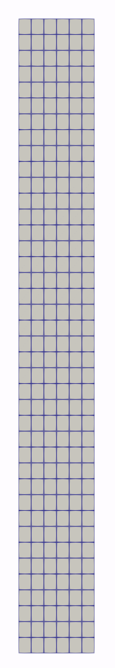
Figure 1: Geometry for Step 1.

Setting the Fluid Properties

Fluid properties are set by first defining a HeliumFluidProperties fluid properties object and second by creating a material that inserts the fluid properties into functors (if you do not know what a functor is then click here).

The first task is performed by the following input syntax:

[FluidProperties]
  [fluid_properties_obj]
    type = HeliumFluidProperties
  []
[]

The second task is performed by the GeneralFunctorFluidProps object:

[FunctorMaterials]
  [fluid_props_to_mat_props]
    type = GeneralFunctorFluidProps
    fp = fluid_properties_obj
    porosity = porosity
    pressure = pressure
    T_fluid = ${T_fluid}
    speed = speed
    characteristic_length = 1
  []
[]

This object takes pressure and temperature provided as variables to parameters pressure and T_fluid, respectively, and computes fluid properties, such as density and viscosity. Density and viscosity are named rho and mu. Note that T_fluid is set to a constant value in this input file because we do not solve the heat equation and therefore have no fluid temperature defined as a variable.

This object also requires providing functors to the porosity, speed, and characteristic_length parameters.

Porosity is defined as an auxiliary variable here:

[AuxVariables]
  [porosity]
    family = MONOMIAL
    order = CONSTANT
    fv = true
    initial_condition = ${bed_porosity}
  []
[]

and set equal to the bed_porosity parameter of 0.39. speed is a functor that is computed automatically by the Navier-Stokes FV action, and characteristic_length is only used for computing Reynolds numbers, which are not required in Step 1; therefore, we set characteristic_length = 1 for now.

Setting up the Thermal-Hydraulics Problem

The thermal-hydraulics problem is set up using the finite volume Navier-Stokes action. This action is discussed in detail here. The corresponding block in the input file is:

[Modules]
  [NavierStokesFV]
    # general control parameters
    compressibility = 'weakly-compressible'
    porous_medium_treatment = true

    # material property parameters
    density = rho
    dynamic_viscosity = mu

    # porous medium treatment parameters
    porosity = porosity

    # initial conditions
    initial_velocity = '1e-6 1e-6 0'
    initial_pressure = 5.4e6

    # boundary conditions
    inlet_boundaries = top
    momentum_inlet_types = fixed-velocity
    momentum_inlet_function = '0 -${flow_vel}'
    wall_boundaries = 'left right'
    momentum_wall_types = 'slip slip'
    outlet_boundaries = bottom
    momentum_outlet_types = fixed-pressure
    pressure_function = ${outlet_pressure}
  []
[]

Understanding the finite volume Navier-Stokes action is important. Therefore, each line will be explained.

    compressibility = 'weakly-compressible'

This line indicates that weakly compressible fluid equations are solved. These equations allow the density of the fluid to vary, and the discretization methods assume Mach numbers of less than 0.2. For compressible flows in reactors, the weakly compressible formulation is the most commonly used equation set.

    porous_medium_treatment = true

    # material property parameters

This line activates the porous flow treatment. Porous flow indicates that fluid and solid share a volume and exchange mass, momentum, and energy in this volume. This exchange is usually described by correlations. In this input file, no mass, momentum, or energy exchange occurs. The porosity defines how much of each porous flow element is fluid. The porosity in this input file is defined as a variable and provided in the line:

    porosity = porosity

    # initial conditions

Note that porosity can also be provided as a functor material property which offers more flexibility when porosity smoothing is required. Porosity smoothing is not used in this tutorial because the Bernoulli treatment for porosity jumps is used. The names of the density and dynamic viscosity functors need to be provided to the action:

    density = rho
    dynamic_viscosity = mu

    # porous medium treatment parameters

Note that these functors are defined by the GeneralFunctorFluidProps object discussed above.

Initial conditions for the velocity and pressure are defined by the lines:

    initial_velocity = '1e-6 1e-6 0'
    initial_pressure = 5.4e6

    # boundary conditions

Note that, since we solve a pseudo-transient, the initial conditions should be interpreted as initial guesses of the solution. We set the initial guess of the velocity to a very small number (this precludes problems that some objects might have with zero velocity) and the initial guess of pressure to MPa. The initial condition for pressure is mismatched with the outlet pressure to make the problem slightly harder to solve.

The boundary conditions are set by these lines:

    inlet_boundaries = top
    momentum_inlet_types = fixed-velocity
    momentum_inlet_function = '0 -${flow_vel}'
    wall_boundaries = 'left right'
    momentum_wall_types = 'slip slip'
    outlet_boundaries = bottom
    momentum_outlet_types = fixed-pressure
    pressure_function = ${outlet_pressure}

The top boundary is the inlet boundary, where we specify the inlet velocity. The inlet velocity is where we note that the velocity is downward, leading to the negative sign. The left and right boundaries are set to slip walls. The bottom boundary is set to a constant pressure outlet.

The relevant values used for substituting the ${variable_name} expressions are computed at the beginning of the input file:

outlet_pressure = 5.5e6
T_fluid = 300
density = 8.60161

mass_flow_rate = 60.0
flow_area = '${fparse pi * bed_radius * bed_radius}'
flow_vel = '${fparse mass_flow_rate / flow_area / density}'

Checking Mass Conservation

We use postprocessors to compute the inlet and outlet mass flow rates.

[Postprocessors]
  [desired_mfr]
    type = Receiver
    default = ${mass_flow_rate}
  []

  [inlet_mfr]
    type = VolumetricFlowRate
    advected_quantity = rho
    vel_x = 'superficial_vel_x'
    vel_y = 'superficial_vel_y'
    boundary = 'top'
    rhie_chow_user_object = pins_rhie_chow_interpolator
  []

  [outlet_mfr]
    type = VolumetricFlowRate
    advected_quantity = rho
    vel_x = 'superficial_vel_x'
    vel_y = 'superficial_vel_y'
    boundary = 'bottom'
    rhie_chow_user_object = pins_rhie_chow_interpolator
  []
[]

The desired_mfr postprocessor simply takes the mass_flow_rate parameter computed at the top of the input file and prints it to screen. This is the mass flow rate we want to achieve.

The inlet_mfr and outlet_mfr are VolumetricFlowRate postprocessors. The VolumetricFlowRate allows the computation of velocity weighted integrals over surfaces. If the advected_quantity is denoted by , velocity by , and the normal on the surface by , then VolumetricFlowRate returns:

For set to density, this is the mass flow rate. We expect all three postprocessors to be identical.

Executioner

The executioner object is explained in detail here. For Step 1 we use these specifications:

[Executioner]
  type = Transient
  end_time = 100
  [TimeStepper]
    type = IterationAdaptiveDT
    iteration_window = 2
    optimal_iterations = 8
    cutback_factor = 0.8
    growth_factor = 2
    dt = 1e-3
  []
  dtmax = 5
  line_search = l2
  solve_type = 'NEWTON'
  petsc_options_iname = '-pc_type -pc_factor_shift_type -pc_factor_mat_solver_package'
  petsc_options_value = 'lu NONZERO superlu_dist'
  nl_rel_tol = 1e-6
  nl_abs_tol = 1e-6
[]

We run a transient to the end_time of 100 seconds. The time steps are selected adaptively based on the number of nonlinear iterations used by the previous timestep. Details on IterationAdaptiveDT can be found here. A maximum timestep of seconds is used. We use Newton's method to solve the problem and solve the linear problem using lower-upper (LU) decomposition. Relative and absolute convergence tolerances are set to .

Results

Execute step1.i by:

./pronghorn-opt -i step1.i

Execution should take about 10 seconds. An exodus file step1_out.e is created. This file contains the pressure and superficial velocity solutions. These are constant at MPa and m/s. Since they are not very relevant, they are not plotted here. The three postprocessors at seconds are:

desired_mfr = 6.000000e+01
inlet_mfr = -5.999997e+01
outlet_mfr = 5.999997e+01

We conserve mass, since inlet_mfr and outlet_mfr are identical. The mass flow rate is also very close to what we expect ( kg/s). The small difference orgininates from truncating the decimals of the assumed density when computing the inlet velocity.