Step 4: Primary Loop
Complete input file for this step: 04_loop.i
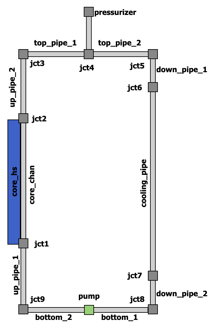
Figure 1: Model diagram
In this step, we will complete the primary loop and set up a simple PID controller for the pump so that it maintains the prescribed mass flow rate.
Close the Loop
We add two pipes for the bottom section of the primary loop with a pump in the middle. A pump is a junction-like component that connects to two flow channels corresponding to its inlet and outlet.
  [jct7]
    type = JunctionOneToOne1Phase
    connections = 'cooling_pipe:out down_pipe_2:in'
  []

  [down_pipe_2]
    type = FlowChannel1Phase
    position = '1 0 0.25'
    orientation = '0 0 -1'
    length = 0.25
    n_elems = 10
    A = ${A_pipe}
    D_h = ${pipe_dia}
  []
The pump component needs 2 more parameters to be specified: reference area A_ref, and head, which is the pump head.
Because the system is now closed, we add a simple pressurizer to maintain the system pressure as the fluid heats up. We split the pipe at the top to create a T-junction with a pipe connected to the pressurizer using a VolumeJunction1Phase. The pressurizer is modeled by prescribing the stagnation pressure with an InletStagnationPressureTemperature1Phase component.
  [jct4]
    type = VolumeJunction1Phase
    position = '0.5 0 2'
    volume = 1e-5
    connections = 'top_pipe_1:out top_pipe_2:in press_pipe:in'
    use_scalar_variables = false
  []

  [press_pipe]
    type = FlowChannel1Phase
    position = '0.5 0 2'
    orientation = '0 0 1'
    length = 0.2
    n_elems = 5
    A = ${A_pipe}
    D_h = ${pipe_dia}
  []

  [pressurizer]
    type = InletStagnationPressureTemperature1Phase
    p0 = ${press}
    T0 = ${T_in}
    input = press_pipe:out
  []
Control Logic
Control logic is a system that allows users to monitor the simulation and change its parameters while it is running.
The system consists of 3 layers:
input layer: which brings values from the simulation inside the control logic system
execution layer: which performs the prescribed operations
output layer: that feeds the values back into simulation
All control logic blocks should be included in the top-level [ControlLogic] block.
Setup PID
A PID control requires several values as an input: set point set_point, input value input, initial value initial_value, and three constants K_p, K_i, and K_d, which are the coefficients for the proportional, integral, and derivative terms, respectively.
For the input value, we set up a postprocessor m_dot_pump with type ADFlowJunctionFlux1Phase which will be measuring the outlet mass flow rate from the pump.
[Postprocessors]
  [m_dot_pump]
    type = ADFlowJunctionFlux1Phase
    boundary = core_chan:in
    connection_index = 1
    equation = mass
    junction = jct7
  []
[]
A set point will be our desired mass flow rate specified by the global parameter m_dot_in. To bring this value into the control logic system, we need to use GetFunctionValueControl block like so:
[ControlLogic]
  [set_point]
    type = GetFunctionValueControl
    function = ${m_dot_in}
  []
[]
This value will be available in the control logic system as set_point:value (in general control_block_name:value).
Then, we add the PID control block as follows:
[ControlLogic]
  [pid]
    type = PIDControl
    initial_value = 0
    set_point = set_point:value
    input = m_dot_pump
    K_p = 1.
    K_i = 4.
    K_d = 0
  []
[]
The value computed by the PID control is available in the control logic system under the name pid:output, where pid is the name of the block.
As a last step, we need to feed this value back into the system. That can be done via SetComponentRealValueControl block.
[ControlLogic]
  [set_pump_head]
    type = SetComponentRealValueControl
    component = pump
    parameter = head
    value = pid:output
  []
[]
The parameter to control is specified via a component and parameter parameters, which are the component name and the parameter name of that component we want to modify.