1D radial heat and mass transport
Description
An analytical solution to the problem of 1D radial coupled heat and mass transport was initially developed by Avdonin (1964), and later by Ross et al. (1982) (in a similar fashion as for the 1D Cartesian model).
The problem consists of a 1D radial model where cold water is injected into a warm semi-infinite reservoir at a constant rate. The top and bottom surfaces of the reservoir are bounded by caprock which is neglected in the modelling to simplify the problem. Instead, these boundaries are treated as no-flow and adiabatic boundary conditions.
For the simple case of a 1D radial model bounded on the upper and lower surfaces by no-flow and adiabatic boundaries, a simplified solution for the temperature profile can be obtained (Updegraff, 1989)
(1)
where is the initial temperature in the reservoir, is the temperature of the injected water, is the gamma function, is the lower incomplete gamma function,
and
where is the density of water, is the specific heat capacity of water, is the density of the fully saturated medium ( where is porosity and is the density of the dry rock), is the specific heat capacity of the fully saturated porous medium, is the thermal conductivity of the fully saturated reservoir, is the volumetric flow rate, and is the height of the reservoir.
Model
This problem was considered in a code comparison by Updegraff (1989), so we use identical parameters in this verification problem, see Table 1.
Table 1: Model properties
| Property | Value |
|---|---|
| Length | 1,000 m |
| Pressure | 5 MPa |
| Temperature | 170 C |
| Permeability | m |
| Porosity | 0.2 |
| Saturate density | 2,500 kg m |
| Saturated thermal conductivity | 25 W m K |
| Saturated specific heat capacity | 1,000 J kg K |
| Mass flux rate | 0.1 kg s |
Input file
The input file used to run this problem is
# Cold water injection into 1D radial hot reservoir (Avdonin, 1964)
#
# To generate results presented in documentation for this problem,
# set xmax = 1000 and nx = 200 in the Mesh block, and dtmax = 1e4
# and end_time = 1e6 in the Executioner block.

[Mesh]
  type = GeneratedMesh
  dim = 1
  nx = 50
  xmin = 0.1
  xmax = 5
  bias_x = 1.05
  rz_coord_axis = Y
  coord_type = RZ
[]

[GlobalParams]
  PorousFlowDictator = dictator
  gravity = '0 0 0'
[]

[AuxVariables]
  [temperature]
    order = CONSTANT
    family = MONOMIAL
  []
[]

[AuxKernels]
  [temperature]
    type = PorousFlowPropertyAux
    variable = temperature
    property = temperature
    execute_on = 'initial timestep_end'
  []
[]

[Variables]
  [pliquid]
    initial_condition = 5e6
  []
  [h]
    scaling = 1e-6
  []
[]

[ICs]
  [hic]
    type = PorousFlowFluidPropertyIC
    variable = h
    porepressure = pliquid
    property = enthalpy
    temperature = 170
    temperature_unit = Celsius
    fp = water
  []
[]

[Functions]
  [injection_rate]
    type = ParsedFunction
    symbol_values = injection_area
    symbol_names = area
    expression = '-0.1/area'
  []
[]

[BCs]
  [source]
    type = PorousFlowSink
    variable = pliquid
    flux_function = injection_rate
    boundary = left
  []
  [pright]
    type = DirichletBC
    variable = pliquid
    value = 5e6
    boundary = right
  []
  [hleft]
    type = DirichletBC
    variable = h
    value = 678.52e3
    boundary = left
  []
  [hright]
    type = DirichletBC
    variable = h
    value = 721.4e3
    boundary = right
  []
[]

[Kernels]
  [mass]
    type = PorousFlowMassTimeDerivative
    variable = pliquid
  []
  [massflux]
    type = PorousFlowAdvectiveFlux
    variable = pliquid
  []
  [heat]
    type = PorousFlowEnergyTimeDerivative
    variable = h
  []
  [heatflux]
    type = PorousFlowHeatAdvection
    variable = h
  []
  [heatcond]
    type = PorousFlowHeatConduction
    variable = h
  []
[]

[UserObjects]
  [dictator]
    type = PorousFlowDictator
    porous_flow_vars = 'pliquid h'
    number_fluid_phases = 2
    number_fluid_components = 1
  []
  [pc]
    type = PorousFlowCapillaryPressureVG
    pc_max = 1e6
    sat_lr = 0.1
    m = 0.5
    alpha = 1e-5
  []
  [fs]
    type = PorousFlowWaterVapor
    water_fp = water
    capillary_pressure = pc
  []
[]

[FluidProperties]
  [water]
    type = Water97FluidProperties
  []
[]

[Materials]
  [watervapor]
    type = PorousFlowFluidStateSingleComponent
    porepressure = pliquid
    enthalpy = h
    temperature_unit = Celsius
    capillary_pressure = pc
    fluid_state = fs
  []
  [porosity]
    type = PorousFlowPorosityConst
    porosity = 0.2
  []
  [permeability]
    type = PorousFlowPermeabilityConst
    permeability = '1.8e-11 0 0 0 1.8e-11 0 0 0 1.8e-11'
  []
  [relperm_water]
    type = PorousFlowRelativePermeabilityCorey
    n = 2
    phase = 0
    s_res = 0.1
    sum_s_res = 0.1
  []
  [relperm_gas]
    type = PorousFlowRelativePermeabilityCorey
    n = 2
    phase = 1
    sum_s_res = 0.1
  []
  [internal_energy]
    type = PorousFlowMatrixInternalEnergy
    density = 2900
    specific_heat_capacity = 740
  []
  [rock_thermal_conductivity]
    type = PorousFlowThermalConductivityIdeal
    dry_thermal_conductivity = '20 0 0  0 20 0  0 0 20'
  []
[]

[Preconditioning]
  [smp]
    type = SMP
    full = true
  []
[]

[Executioner]
  type = Transient
  solve_type = NEWTON
  end_time = 1e3
  nl_abs_tol = 1e-8
  [TimeStepper]
    type = IterationAdaptiveDT
    dt = 100
  []
[]

[Postprocessors]
  [injection_area]
    type = AreaPostprocessor
    boundary = left
    execute_on = initial
  []
[]

[VectorPostprocessors]
  [line]
    type = ElementValueSampler
    sort_by = x
    variable = temperature
    execute_on = 'initial timestep_end'
  []
[]

[Outputs]
  perf_graph = true
  [csv]
    type = CSV
    execute_on = final
  []
[]
Note that the test file is a reduced version of this problem. To recreate these results, follow the instructions at the top of the input file.
Results
The results for the temperature profile after 13,000 seconds are shown in Figure 1. Excellent agreement between the analytical solution and the MOOSE results are observed.
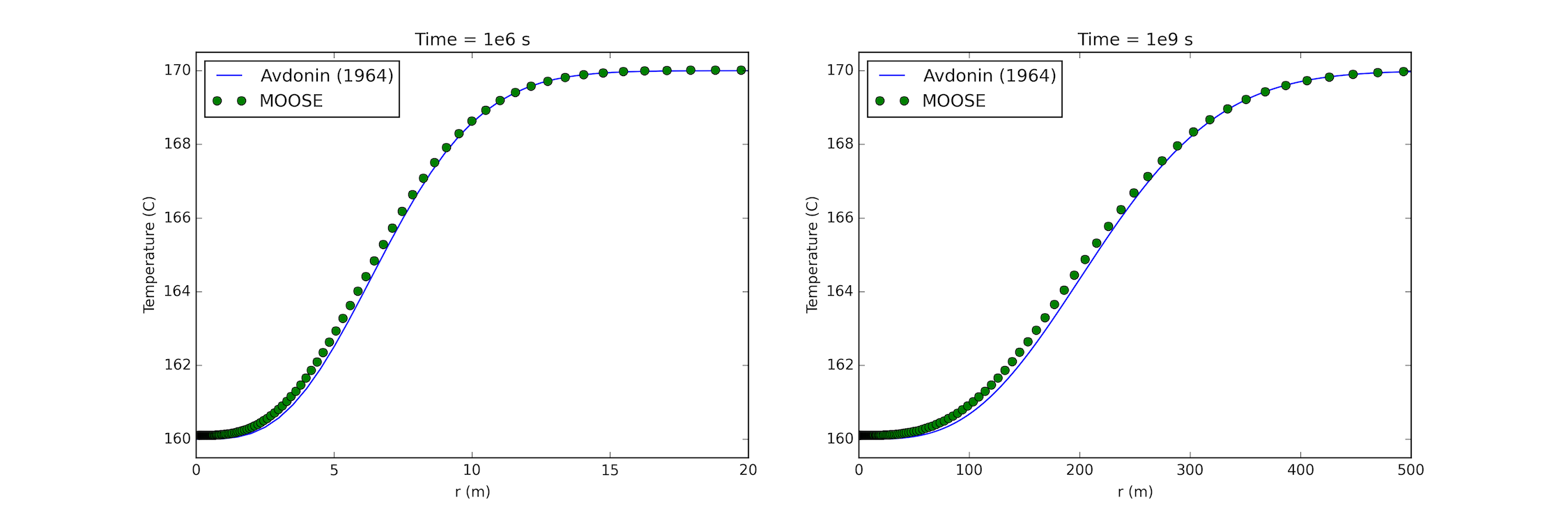
Figure 1: Comparison between Avdonin (1964) result and MOOSE at s (left); and s (right).
This model also admits a similarity solution (Moridis and Pruess, 1992). Again, excellent agreement between the analytical solution and the MOOSE results are observed, see Figure 2
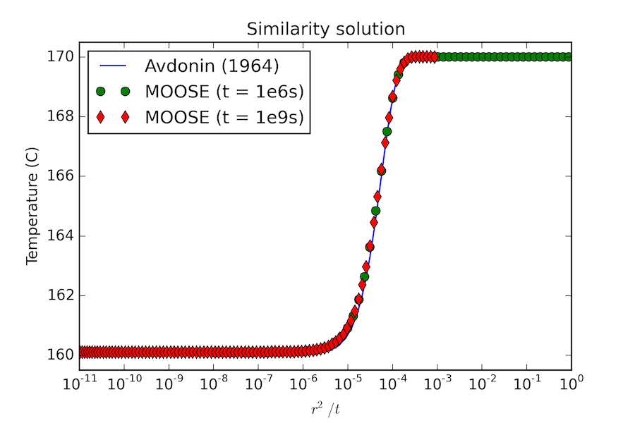
Figure 2: Similarity solution for 1D radial problem.
References
- NA Avdonin.
Some formulas for calculating the temperature field of a stratum subject to thermal injection.
Neft'i Gaz, 3:37–41, 1964.[BibTeX]
- GJ Moridis and K Pruess.
Tough simulations of updegraff's set of fluid and heat flow problems.
LBL-32611, Lawrence Berkeley Lab, 1992.[BibTeX]
- B Ross, JW Mercer, SD Thomas, and BH Lester.
Benchmark problems for repository siting models.
Technical Report, GeoTrans, 1982.[BibTeX]
- C David Updegraff.
Comparison of strongly heat-driven flow codes for unsaturated media.
Technical Report, Nuclear Regulatory Commission, 1989.[BibTeX]