Flow and Solute Transport in Porous Media
1D solute transportation
Problem statement
This example is based on Karmakar et al. (2022). The transportation of tracer in water in a 1D porous tank is modelled. The schematic is demonstrated in Figure 1. The experiment details are elaborated in the referred paper so will not be shown here to avoid repetition. The governing equations are provided below:
(1)
(2)
Notation used in these equations is summarised in the nomenclature.
Table 1: Parameters of the problem .
| Symbol | Quantity | Value | Units |
|---|---|---|---|
| Porosity | |||
| Permeability | |||
| Viscosity () | |||
| Gravity | |||
| Initial temperature | |||
| Total time | days |
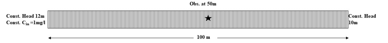
Figure 1: The schematic of the problem Karmakar et al. (2022).
Input file setup
This section describes the input file syntax.
Mesh
The first step is to set up the mesh. In this problem, a tank with a length of 100 m is simulated and an element size of 1 m is used.
[Mesh]
  [gen]
    type = GeneratedMeshGenerator
    dim = 1
    nx = 100
    xmin = 0
    xmax = 100
  []
[]
Fluid properties
After the mesh has been specified, we need to provide the fluid properties that are used for this simulation. For our case, it will be just water and can be easily implemented as follows:
[FluidProperties]
  [water]
    type = Water97FluidProperties
  []
[]
Variables declaration
Then, we need to declare what type of unknown we are solving. This can be done in the variable code block. Since we are focusing on the concentration of tracer at x =50 m, C is a desired variable. Porepressure is also used for the fluid motion. Since we only have constant initial conditions so they can be directly supplied here.
[Variables]
  [porepressure]
    initial_condition = 1e5
  []
  [C]
    initial_condition = 0
  []
[]
Kernel declaration
This section describes the physics we need to solve. To do so, some kernels are declared. In MOOSE, the required kernels depend on the terms in the governing equations. For this problem, six kernels were declared. To have a better understanding, users are recommended to visit this page. The code block is shown below with the first three kernels associated with equation 1 and the remain associated with equation 2.
[Kernels]
  [mass_der_water]
    type = PorousFlowMassTimeDerivative
    fluid_component = 1
    variable = porepressure
  []
  [adv_pp]
    type = PorousFlowFullySaturatedDarcyFlow
    variable = porepressure
    fluid_component = 1
  []
  [diff_pp]
    type = PorousFlowDispersiveFlux
    fluid_component = 1
    variable = porepressure
    disp_trans = 0
    disp_long = ${disp}
  []
  [mass_der_C]
    type = PorousFlowMassTimeDerivative
    fluid_component = 0
    variable = C
  []
  [adv_C]
    type = PorousFlowFullySaturatedDarcyFlow
    fluid_component = 0
    variable = C
  []
  [diff_C]
    type = PorousFlowDispersiveFlux
    fluid_component = 0
    variable = C
    disp_trans = 0
    disp_long = ${disp}
  []
[]
Material setup
Additional material properties are required , which are declared here:
[Materials]
  [ps]
    type = PorousFlow1PhaseFullySaturated
    porepressure = porepressure
  []
  [porosity]
    type = PorousFlowPorosityConst
    porosity = 0.25
  []
  [permeability]
    type = PorousFlowPermeabilityConst
    permeability = '1E-11 0 0   0 1E-11 0   0 0 1E-11'
  []
  [water]
    type = PorousFlowSingleComponentFluid
    fp = water
    phase = 0
  []
  [massfrac]
    type = PorousFlowMassFraction
    mass_fraction_vars = C
  []
  [temperature]
    type = PorousFlowTemperature
    temperature = 293
  []
  [diff]
    type = PorousFlowDiffusivityConst
    diffusion_coeff = '0 0'
    tortuosity = 0.1
  []
  [relperm]
    type = PorousFlowRelativePermeabilityConst
    kr = 1
    phase = 0
  []
[]
Boundary Conditions
The next step is to supply the boundary conditions. There are three Dirichlet boundary conditions that we need to supply. The first two are constant pressure at the inlet and outlet denoted as constant_inlet_pressure and constant_outlet_porepressure. Another one is constant tracer concentration at the inlet denoted as inlet_tracer. Finally, a PorousFlowOutflowBC boundary condition was supplied at the outlet to allow the tracer to freely move out of the domain.
[BCs]
  [constant_inlet_pressure]
    type = DirichletBC
    variable = porepressure
    value = 1.2e5
    boundary = left
  []
  [constant_outlet_porepressure]
    type = DirichletBC
    variable = porepressure
    value = 1e5
    boundary = right
  []
  [inlet_tracer]
    type = DirichletBC
    variable = C
    value = 0.001
    boundary = left
  []
  [outlet_tracer]
    type = PorousFlowOutflowBC
    variable = C
    boundary = right
    mass_fraction_component = 0
  []
[]
Executioner setup
For this problem, a transient solver is required. To save time and computational resources, IterationAdaptiveDT was implemented. This option enables the time step to be increased if the solution converges and decreased if it does not. Thus, this will help save time if a large time step can be used and aid in convergence if a small time step is required. For practice, users can try to disable it by putting the code block into comment and witnessing the difference in the solving time and solution.
[Executioner]
  type = Transient
  end_time = 17280000
  dtmax = 86400
  nl_rel_tol = 1e-6
  nl_abs_tol = 1e-12
  [TimeStepper]
    type = IterationAdaptiveDT
    dt = 1000
  []
[]
Auxiliary kernels and variables (optional)
This section is optional since these kernels and variables do not affect the calculation of the desired variable. In this example, we want to know the Darcy velocity in the x direction thus we will add an auxkernel and an auxvariable for it.
[AuxVariables]
  [Darcy_vel_x]
    order = CONSTANT
    family = MONOMIAL
  []
[]
[AuxKernels]
  [Darcy_vel_x]
    type = PorousFlowDarcyVelocityComponent
    variable = Darcy_vel_x
    component = x
    fluid_phase = 0
  []
[]
Postprocessor
As previously discussed, we only want to know the variation of concentration (C) and x-direction Darcy velocity at x=50 m over time. So, we need to tell MOOSE to only write that information into the result file via this code block.
[Postprocessors]
  [C]
    type = PointValue
    variable = C
    point = '50 0 0'
  []
  [Darcy_x]
    type = PointValue
    variable = Darcy_vel_x
    point = '50 0 0'
  []
[]
Result
The results obtained from MOOSE are compared against the analytical solution proposed by Ogata et al. (1961).
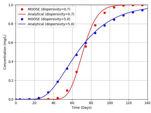
Figure 2: Tracer concentration with respect to time.
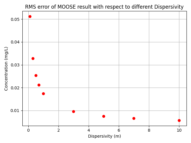
Figure 3: Root-mean-square error of MOOSE results.
Compared with the benchmark conducted by Karmakar et al. (2022), it can be seen that MOOSE is capable of delivering accurate results for this type of problem.
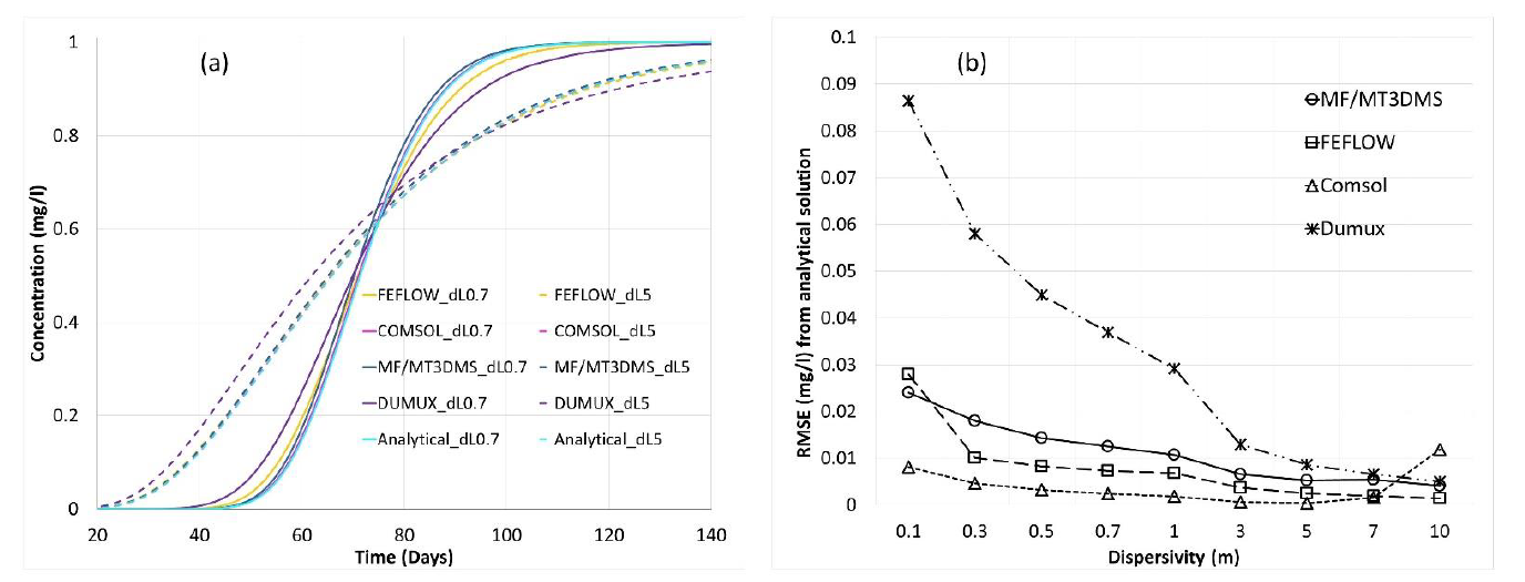
Figure 4: The benchmark conducted by Karmakar et al. (2022).
2D solute transportation
Problem statement
This example is based on Karmakar et al. (2022). The transportation of tracer in water in a 2D porous tank is modelled. The schematic is demonstrated in Figure 5. The parameters are the same as the 1D problem as provided in Table 1.
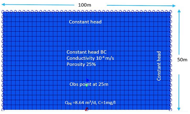
Figure 5: The schematic of the 2D problem Karmakar et al. (2022).
Input file setup
The input file for this problem is similar to the 1D case except for some changes made to account for the 2D mesh and the changes in the boundary conditions which are elaborated in the following sections. Other sections will be the same as the 1D case.
Mesh
For this problem, to simulate a 2D rectangular aquifer with a point source placed at the origin, the x-domain was chosen from -50 to 50 m and the y-domain from 0 to 50 m.
[Mesh]
  [gen]
    type = GeneratedMeshGenerator
    dim = 2
    nx = 100
    xmin = -50
    xmax = 50
    ny = 60
    ymin = 0
    ymax = 50
  []
[]
DiracKernels set-up
Since our problem comprises a point source, PorousFlowSquarePulsePointSource DiracKernels are required. These DiracKernels inject the water and tracer into the domain at a constant rate. As can be seen below, two DiracKernels are used. The first one supplies the water with a specified mass flux to the system and the second one the tracer.
[DiracKernels]
  [source_P]
    type = PorousFlowSquarePulsePointSource
    point = '0 0 0'
    mass_flux = 1e-1
    variable = porepressure
  []
  [source_C]
    type = PorousFlowSquarePulsePointSource
    point = '0 0 0'
    mass_flux = 1e-7
    variable = C
  []
[]
Boundary Conditions
The boundary conditions are similar to the 1D case except for the addition of several Dirichlet, and outflow conditions due to the extra faces of the 2D problem. The bottom face was not supplied with any boundary condition as it a line of symmetry (only half the model is simulated). Therefore, no-flow is allowed across this boundary.
[BCs]
  [constant_outlet_porepressure_]
    type = DirichletBC
    variable = porepressure
    value = 1e5
    boundary = 'top left right'
  []
  [outlet_tracer_top]
    type = PorousFlowOutflowBC
    variable = C
    boundary = top
    mass_fraction_component = 0
  []
  [outlet_tracer_right]
    type = PorousFlowOutflowBC
    variable = C
    boundary = right
    mass_fraction_component = 0
  []
  [outlet_tracer_left]
    type = PorousFlowOutflowBC
    variable = C
    boundary = left
    mass_fraction_component = 0
  []
[]
Result
The results obtained from MOOSE are compared against the analytical solution proposed by Schroth et al. (2000).
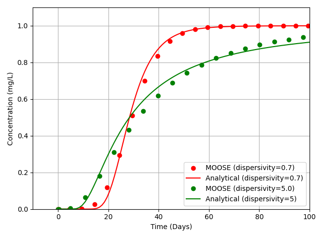
Figure 6: Tracer concentration with respect to time.
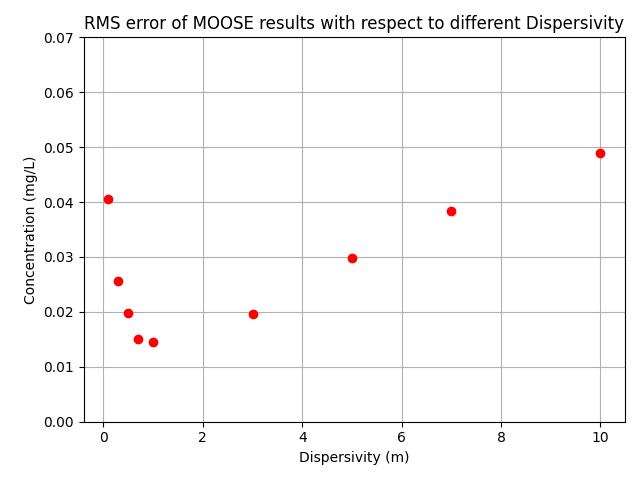
Figure 7: Root-mean-square error of MOOSE results.
Compared with the benchmark conducted by Karmakar et al. (2022), it can be seen that once again MOOSE is capable of delivering accurate results for this type of problem.
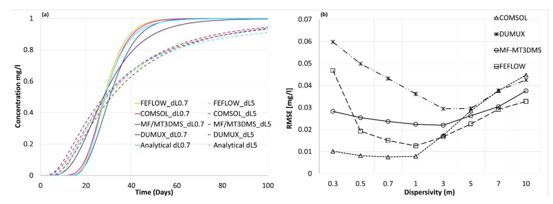
Figure 8: The benchmark conducted by Karmakar et al. (2022).
References
- Shyamal Karmakar, Alexandru Tatomir, Sandra Oehlmann, Markus Giese, and Martin Sauter.
Numerical benchmark studies on flow and solute transport in geological reservoirs.
Water, 2022.
URL: https://www.mdpi.com/2073-4441/14/8/1310, doi:10.3390/w14081310.[BibTeX]
- Akio Ogata, Robert B. Banks, Stewart Lee Udall, and Thomas B Nolan.
A solution of the differential equation of longitudinal dispersion in porous media.
Technical Report, United States Department of the Interior, 1961.
URL: https://api.semanticscholar.org/CorpusID:117806845.[BibTeX]
- M.H Schroth, Jonathan Istok, and Roy Haggerty.
In situ evaluation of solute retardation using single-well push–pull tests.
Advances in Water Resources, 24:105–117, 10 2000.
doi:10.1016/S0309-1708(00)00023-3.[BibTeX]