Compute efficiencies
Geochemistry simulations use a large amount of memory since they store information about a complete geochemical system at each finite-element node, and, optionally, populate a huge number of AuxVariables with useful information. On the other hand, ignoring transport, they are almost embarrassingly parallel, so may be solved efficiently using a large number of processors.
This page explores computational aspects of the 2D GeoTES simulation, the Weber-Tensleep GeoTES simulation and the FORGE geothermal simulation which are coupled porous-flow + geochemistry simulations.
Memory usage for pure geochemistry simulations
While spatially-dependent geochemistry simulations are rarely run without transport, it is useful to quantify the amount of memory used by geochemistry models alone (without transport) because memory consumption can easily swamp all other considerations. Table 1 lists the numbers of species in the two simulations used in this section.
Table 1: Size of the two simulations
| 2D | Weber-Tensleep | |
|---|---|---|
| Basis species | 4 | 20 |
| Secondary species | 1 | 166 |
| Minerals | 1 | 15 |
| Total species () | 6 | 201 |
The Geochemistry Actions, such as the SpatialReactionSolver, add a large number of AuxVariables by default. These record the species' molality, free mass, free volume, activity, bulk composition, etc, which may be useful but add considerably to the memory consumption. Some examples are quantified in Table 2 and Table 3.
Table 2: Memory used by the 2D geochemistry-only simulation
| Number of nodes () | MB with Zero AuxVariables () | MB with 24 AuxVariables () |
|---|---|---|
| 1181 | 56 | 61 |
| 3333 | 63 | 71 |
| 6633 | 80 | 93 |
| 13233 | 114 | 139 |
| 26433 | 183 | 229 |
Table 3: Memory used by the Weber-Tensleep geochemistry-only simulation
| Number of nodes () | MB with 6 AuxVariables () | MB with 770 AuxVariables () |
|---|---|---|
| 480 | 94 | 227 |
| 930 | 130 | 290 |
| 1830 | 204 | 416 |
| 3630 | 351 | 667 |
| 7230 | 582 | 1171 |
The results are summarised in the approximate formula where is the number of nodes, the number of species ( and in the two examples) and the number of AuxVariables.
The first term is largely independent of
geochemistryso is not too important here.The second term depends on the size of the geochemical system, , and quantifies the cost of keeping track of an entire geochemical at each node, which is approximately bytes per node. Recall that is the total number of species in the geochemical model.
The third term depends on the size of the Auxiliary system, which is approximately bytes per node. Recall that this is about if all the default AuxVariables are added by the Action.
Of course, the memory consumption will be dependent on the compiler and architecture, but the above formula should provide an approximate guide.
Compute time for pure geochemistry simulations
The geochemistry-only part of the FORGE geothermal simulation (aquifer_geochemistry.i with 15251 nodes and no exodus output) may be run using a different number of processors in order to demonstrate the computational efficiencies of pure geochemistry simulations that have no transport. (In fact, exactly the same computations are performed at each node in this case, but MOOSE does not know this.) As is evident from Table 4 and Figure 1, geochemical-only simulations scale very well with the number of processors.
Table 4: Compute time (s) for the FORGE geothermal simulation using different numbers of processors
| Number of processors | Time required (s) |
|---|---|
| 1 | 2001 |
| 2 | 1010, 1011, 1010 |
| 4 | 533, 531, 534 |
| 6 | 387, 409, 399 |
| 8 | 298, 313, 317 |
| 10 | 233, 236, 241 |
| 16 | 156, 157, 158 |
| 20 | 132, 144, 135, 132 |
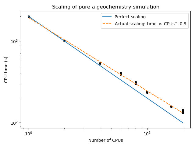
Figure 1: CPU time required to solve the FORGE geochemistry-only simulation with no transport.
Relative compute-time spent in transport and reactions
It is common that the "reaction" part of reactive-transport simulations proceeds quickly compared with the transport part. This is because the geochemistry module bypasses a lot of MOOSE overhead and because there are no spatial derivatives that require the use of PETSc. Table 5 quantifies this for the FORGE example and an example from the geochemistry test suite. Although this is just one example, the large cost of a full PorousFlow solve is evident. If possible, compute time will be reduced by pre-computing the Darcy velocity and time-dependent temperature field and using these in the GeochemistryTimeDerivative and ConservativeAdvection Kernels, as in the advection_1.i input file.
Table 5: Compute time (s) for various parts of a typical reactive-transport simulation. The mesh in each case has 1886 nodes, and 20 time steps are run using a single processor.
| Simulation | Time required (s) | Notes |
|---|---|---|
FORGE aquifer_geochemistry.i | 14 | 11 basis species, 14 kinetic minerals, 181056 AuxVariables |
FORGE porous_flow.i | 90 | 12 Variables, 22632 DoFs, 20746 AuxVariables. The simulation needs approximately 2 Nonlinear iterations per time-step and uses ILU |
| Above two combined in a MultiApp | 97 | Enhanced efficiency compared with because porous_flow.i demands small timesteps so aquifer_geochemistry.i does little work |
Test advection_1.i with modified mesh and 12 "conc" variables | 28 | 12 Variables, 22632 DoFs, 3600 AuxVariables. The simulation needs approximately 2 Nonlinear iterations per time-step and uses ILU |
Solver choices for simulations coupled with PorousFlow
Geochemistry simulations are often coupled with PorousFlow in order to simulate reactive transport. The previous section demonstrated that the "transport" part of such simulations is likely to be much more expensive than the "reactive" part. Hence, it is useful to explore ways of improving its efficiency. One way is to pre-compute the Darcy velocity and temperature field, and use the GeochemistryTimeDerivative and ConservativeAdvection Kernels. However, this is often not possible. Therefore, this section quantifies the compute time required for a typical PorousFlow simulation.
A 2D example
The FORGE porous_flow.i input file is used with mesh defined by
    type = GeneratedMeshGenerator
    dim = 2
    nx = 135
    ny = 120
    xmin = -400
    xmax = 500
    ymin = -400
    ymax = 400
This leads to 197472 DoFs, which splits nicely over 20 processors to yield about 10000 DoFs per processor. The simulation is run for 20 time-steps, most of which converge in 2 Nonlinear iterations. Table 6 shows that there are a variety of solver and preconditioner choices that provide fairly comparable performance, but that there are some that are quite poor. The results are for only one 2D model, but it is useful to note that hypre, FSP, ASM + ILU and bjacobi all perform similarly, and that complicated features such as the asm_overlap, asm_shift_type, diagonal_scale and diagonal_scale_fix, and very strong preconditioners like MUMPS are not beneficial in these types of simulations, in contrast to multi-phase PorousFlow models.
Table 6: Compute time (s) for 20 time-steps of the 2D porous_flow.i simulations run over 20 processors with about 10000 DoFs per processor. Note that the time required is only accurate to within about 5% due to the vagaries of HPC.
| Time required (s) | Preconditioner | Notes |
|---|---|---|
| 51 | hypre | Using the boomeramg type with default options |
| 59 | hypre | Using boomeramg and choosing max_levels = 2 |
| 51 | hypre | Using boomeramg and choosing max_levels >= 4 |
| 51 – 57 | hypre | Using boomeramg and varying max_iter between 2 (fastest) and 5 (slowest) |
| 51 | hypre | Using boomeramg with various levels of strong_threshold |
| 53 | BJACOBI | With the GMRES KSP method |
| 52 | FSP | Fieldsplit with being the mass fractions and temperature, and being porepressure, and using hypre + gmres for each subsystem, and splitting_type additive or multiplicative |
| 56 | ASM + ILU | With the GMRES KSP method. Virtually independent of asm_overlap. Not needed: nonzero shift_type, diagonal_scale and diagonal_scale_fix |
| 56 | ASM + ILU | With the BCGS KSP method |
| 57 | SOR | With default options |
| 58 | FSP | Fieldsplit with being the mass fractions and temperature, and being porepressure, and using hypre + gmres for each subsystem, and splitting_type schur |
| 94 | LU | With the GMRES KSP method |
| 94 | LU | Using MUMPS |
| 109 | ASM + LU | With the GMRES KSP method |
| 116 | ASM + ILU | With the TFQMR KSP method |
| 124 | FSP | Fieldsplit with being the mass fractions, and being porepressure and temperature, and using hypre + gmres for each subsystem |
The fieldsplit preconditioning is a little more complicated than simply setting pc_type = hypre, pc_hypre_type = boomeramg. Here is a sample block:
[Preconditioning]
  [FSP]
    type = FSP
    topsplit = 'up' # 'up' should match the following block name
    [up]
      splitting = 'u p' # 'u' and 'p' are the names of subsolvers, below
      splitting_type  = multiplicative
      petsc_options_iname = '-pc_fieldsplit_schur_fact_type  -pc_fieldsplit_schur_precondition'
      petsc_options_value = 'full selfp'
    []
    [u]
      vars = 'f_H f_Na f_K f_Ca f_Mg f_SiO2 f_Al f_Cl f_SO4 f_HCO3 temperature'
      petsc_options_iname = '-pc_type -ksp_type'
      petsc_options_value = ' hypre    gmres'
    []
    [p]
      vars = 'porepressure'
      petsc_options_iname = '-pc_type -ksp_type'
      petsc_options_value = ' hypre    gmres'
    []
  []
[]
A 3D example
The FORGE porous_flow.i input file used with mesh defined by
    type = GeneratedMeshGenerator
    dim = 3
    nx = 36
    ny = 32
    nz = 10
    xmin = -400
    xmax = 500
    ymin = -400
    ymax = 400
This leads to 161172 DoFs, which splits nicely over 20 processors to yield about 10000 DoFs per processor. The simulation is run for 10 time-steps, most of which converge in 2 Nonlinear iterations. Table 7 shows that there are a variety of solver and preconditioner choices that provide fairly comparable performance, but some are quite poor. The results are for only one 3D model, but it is useful to note that hypre is the best by a significant margin, followed by FSP + hypre + gmres and ASM + ILU. Complicated features such as the asm_overlap, asm_shift_type, diagonal_scale and diagonal_scale_fix, and strong preconditioners like ASM + LU or MUMPS add extra overhead in these types of simulations, in contrast to multi-phase PorousFlow models.
Table 7: Compute time (s) for 10 time-steps of the 3D porous_flow.i simulations run over 20 processors with about 10000 DoFs per processor. Each simulation uses the GMRES KSP method with restart = 300. Note that the time required is only accurate to within about 5% due to the vagaries of HPC.
| Time required (s) | Preconditioner | Notes |
|---|---|---|
| 100 | hypre | Using the boomeramg type with default options |
| 170 | FSP | Fieldsplit with being the mass fractions and temperature, and being porepressure, and using hypre + gmres for each subsystem, and splitting_type multiplicative |
| 200 | ASM + ILU | asm_overlap = 0 |
| 250 | ASM + ILU | asm_overlap = 0 and asm_shift_type = NONZERO and -ksp_diagonal_scale -ksp_diagonal_scale_fix |
| 300 | BJACOBI | |
| 472 | ASM + LU | With asm_overlap = 0 |
| 580 | ASM + LU | With asm_overlap = 1 |
| >1000 | ASM + ILU | asm_overlap = 1 |
| >1000 | ASM + LU | With asm_overlap = 2 |
| >1000 | LU | Using MUMPS |
Enthusiastic readers will play with further choices (for instance, Eisenstat-Walker options) but it is hoped the above tables will provide a useful starting point.
Reactive-transport using multiple processors
A large reactive-transport simulation based on the 2D FORGE model is used to study the scaling behaviour with the number of processors. Given the above results, this is mainly testing the scaling behaviour of the linear solver for the PorousFlow simulation. The mesh used is
    type = GeneratedMeshGenerator
    dim = 2
    nx = 450
    ny = 400
    xmin = -400
    xmax = 500
    ymin = -400
    ymax = 400
The magnitude of the problem is tabulated in Table 8. The simulation is run for 100 time-steps using the hypre boomeramg preconditioner in porous_flow.i.
Table 8: Size of the large reactive-transport 2D simulation.
| Parameter | Number |
|---|---|
| Nodes | 180851 |
| Elements | 180000 |
| PorousFlow DoFs | 2170212 |
| PorousFlow AuxVariables DoFs | 1989361 |
| Geochemistry basis species | 11 |
| Geochemistry kinetic species | 14 |
| Geochemistry AuxVariable DoFs | 17361696 |
The results are tabulated in Table 9 and Figure 1
Table 9: Size of the large reactive-transport 2D simulation.
| Number of processors | Walltime (s) |
|---|---|
| 10 | 6253 |
| 20 | 3310 |
| 40 | 2028 |
| 60 | 1216 |
| 80 | 960 |
| 100 | 830 |
| 140 | 606 |
| 200 | 470 |
Figure 2: CPU time required to solve the FORGE reactive-transport simulation involving a MultiApp coupling between PorousFlow and Geochemistry.