Simulating a simple GeoTES experiment
This page describes a reactive-transport simulation of a simple GeoTES scenario. The transport is handled using the PorousFlow module, while the Geochemistry module is used to simulate a heat exchanger and the geochemistry. The simulations are coupled together in an operator-splitting approach using MultiApps.
In Geological Thermal Energy Storage (GeoTES), hot fluid is pumped into an subsurface confined aquifer, stored there for some time, then pumped back again to produce electricity. Many different scenarios have been proposed, including different borehole geometries (used to pump the fluid), different pumping strategies and cyclicities (pumping down certain boreholes, up other boreholes, etc), different temperatures, different aquifer properties, etc. This page only describes the heating phase of a particularly simple set up.
Two wells (boreholes) are used.
The cold (production) well, which pumps aquifer water from the aquifer.
The hot (injection) well, which pumps hot fluid into the aquifer.
These are connected by a heat-exchanger, which heats the aquifer water produced from (1) and passes it to (2). This means the fluid pumped through the injection well is, in fact, heated aquifer water, which is important practically from a water-conservation standpoint, and to assess the geochemical aspects of circulating aquifer water through the GeoTES system.
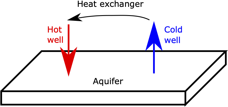
Figure 1: Schematic of the simple GeoTES simulation.
Aquifer geochemistry
It is assumed that only HO, Na, Cl and SiO(aq) are present in the system. While this is unrealistically simple for any aquifer, it allows this page to focus on the method of constructing more complicated models avoiding rather lengthy input files.
The database file
A small geochemical database involving only these species is used. Readers who are building their own database might find exploring its structure useful:
{
  "Header": {
    "title": "Very small MOOSE thermodynamic database",
    "original": "moose/modules/geochemistry/python/original_dbs/gwb_llnl.dat",
    "date": "09:14 18-08-2020",
    "original format": "gwb",
    "activity model": "debye-huckel",
    "fugacity model": "tsonopoulos",
    "logk model": "fourth-order",
    "logk model (functional form)": "a0 + a1 T + a2 T^2 + a3 T^3 + a4 T^4",
    "temperatures": [
      0.0,
      25.0,
      60.0,
      100.0,
      150.0,
      200.0,
      250.0,
      300.0
    ],
    "pressures": [
      1.0134,
      1.0134,
      1.0134,
      1.0134,
      4.76,
      15.549,
      39.776,
      85.927
    ],
    "adh": [
      0.4913,
      0.5092,
      0.545,
      0.5998,
      0.6898,
      0.8099,
      0.9785,
      1.2555
    ],
    "bdh": [
      0.3247,
      0.3283,
      0.3343,
      0.3422,
      0.3533,
      0.3655,
      0.3792,
      0.3965
    ],
    "bdot": [
      0.0174,
      0.041,
      0.044,
      0.046,
      0.047,
      0.047,
      0.034,
      0.0
    ],
    "neutral species": {
      "co2": {
        "a": [
          0.1224,
          0.1127,
          0.09341,
          0.08018,
          0.08427,
          0.09892,
          0.1371,
          0.1967
        ],
        "b": [
          -0.004679,
          -0.01049,
          -0.0036,
          -0.001503,
          -0.01184,
          -0.0104,
          -0.007086,
          -0.01809
        ],
        "c": [
          -0.0004114,
          0.001545,
          9.609e-05,
          0.0005009,
          0.003118,
          0.001386,
          -0.002887,
          -0.002497
        ],
        "d": [
          0.0,
          0.0,
          0.0,
          0.0,
          0.0,
          0.0,
          0.0,
          0.0
        ]
      },
      "h2o": {
        "a": [
          1.4203,
          1.45397,
          1.5012,
          1.5551,
          1.6225,
          1.6899,
          1.7573,
          1.8247
        ],
        "note": "Missing array values in original database have been filled using a linear fit. Original values are [500.0000, -.0005362, 500.0000, -.0007132, -.0008312, 500.0000, 500.0000, 500.0000]",
        "b": [
          0.0177,
          0.022357,
          0.0289,
          0.036478,
          0.045891,
          0.0553,
          0.0647,
          0.0741
        ],
        "c": [
          0.0103,
          0.0093804,
          0.008,
          0.0064366,
          0.0045221,
          0.0026,
          0.0006,
          -0.0013
        ],
        "d": [
          -0.0005,
          -0.0005362,
          -0.0006,
          -0.0007132,
          -0.0008312,
          -0.0009,
          -0.0011,
          -0.0012
        ]
      }
    }
  },
  "elements": {
    "Cl": {
      "name": "Chlorine",
      "molecular weight": 35.453
    },
    "H": {
      "name": "Hydrogen",
      "molecular weight": 1.0079
    },
    "Na": {
      "name": "Sodium",
      "molecular weight": 22.9898
    },
    "O": {
      "name": "Oxygen",
      "molecular weight": 15.9994
    },
    "Si": {
      "name": "Silicon",
      "molecular weight": 28.085
    }
  },
  "basis species": {
    "H2O": {
      "elements": {
        "H": 2.0,
        "O": 1.0
      },
      "radius": 0.0,
      "charge": 0.0,
      "molecular weight": 18.0152
    },
    "Cl-": {
      "elements": {
        "Cl": 1.0
      },
      "radius": 3.0,
      "charge": -1.0,
      "molecular weight": 35.453
    },
    "Na+": {
      "elements": {
        "Na": 1.0
      },
      "radius": 4.0,
      "charge": 1.0,
      "molecular weight": 22.9898
    },
    "SiO2(aq)": {
      "elements": {
        "O": 2.0,
        "Si": 1.0
      },
      "radius": -0.5,
      "charge": 0.0,
      "molecular weight": 60.0843
    }
  },
  "secondary species": {
    "NaCl": {
      "species": {
        "Na+": 1.0,
        "Cl-": 1.0
      },
      "charge": 0.0,
      "radius": 4.0,
      "molecular weight": 58.4428,
      "logk": [
        1.855,
        1.5994,
        1.2945,
        0.9856,
        0.635,
        0.2935,
        -0.0407,
        -0.3487
      ],
      "note": "Missing array values in original database have been filled using a fourth-order fit. Original values are [1.8550, 1.5994, 1.2945, .9856, .6350, .2935, 500.0000, 500.0000]"
    }
  },
  "free electron": {
    "e-": {
      "species": {
        "H2O": 0.5,
        "O2(g)": -0.25,
        "H+": -1.0
      },
      "charge": -1.0,
      "radius": 0.0,
      "molecular weight": 0.0,
      "logk": [
        22.76135,
        20.7757,
        18.513025,
        16.4658,
        14.473225,
        12.92125,
        11.68165,
        10.67105
      ]
    }
  },
  "mineral species": {
    "QuartzLike": {
      "species": {
        "SiO2(aq)": 1.0
      },
      "molar volume": 22.688,
      "molecular weight": 60.0843,
      "logk": [-5.0, -4.0, -3.0, -2.0, -1.0, 0.0, 1.0, 2.0]
    },
    "QuartzUnlike": {
      "species": {
        "SiO2(aq)": 1.0
      },
      "molar volume": 22.688,
      "molecular weight": 60.0843,
      "logk": [-1.0, -2.0, -3.0, -4.0, -5.0, -6.0, -7.0, -8.0]
    }
  }
}
Initial conditions
The aquifer temperature is uniformly 50C before injection and production.
The aquifer is assumed to be consist entirely of a mineral called QuartzLike and a kinetic rate is used for its dissolution. The mineral QuartzLike is similar to Quartz but it has a different equilibrium constant structure in order to emphasise the dissolution upon heating.
Each 1kg of solvent water is assumed to hold 0.1mol of Na and Cl, and a certain amount of SiO(aq). The following input file finds the free molality of SiO(aq) when in contact with QuartzLike at 50C:
# Finds the equilibrium free molality of SiO2(aq) when in contact with QuartzLike at 50degC
[UserObjects]
  [definition]
    type = GeochemicalModelDefinition
    database_file = "small_database.json"
    basis_species = "H2O SiO2(aq) Na+ Cl-"
    equilibrium_minerals = "QuartzLike"
  []
[]

[TimeIndependentReactionSolver]
  model_definition = definition
  geochemistry_reactor_name = reactor
  charge_balance_species = "Cl-"
  swap_out_of_basis = "SiO2(aq)"
  swap_into_basis = QuartzLike
  constraint_species = "H2O              Na+              Cl-              QuartzLike"
  constraint_value = "  1.0              0.1              0.1              396.685" # amount of QuartzLike is unimportant (provided it is positive).  396.685 is used simply because the other geotes_2D input files use this amount
  constraint_meaning = "kg_solvent_water bulk_composition bulk_composition free_mineral"
  constraint_unit = "   kg               moles            moles            moles"
  temperature = 50.0
  ramp_max_ionic_strength_initial = 0 # max_ionic_strength in such a simple problem does not need ramping
  add_aux_pH = false # there is no H+ in this system
  precision = 12
[]

[Postprocessors]
  [free_moles_SiO2]
    type = PointValue
    point = '0 0 0'
    variable = 'molal_SiO2(aq)'
  []
[]

[Outputs]
  csv = true
[]
The result it molality = 0.000555052386. It is necessary to find this initial molality, only because QuartzLike is a kinetic species, so cannot appear the basis (see another similar example). If it were treated as an equilibrium species, its initial free mole number could be specified in the input file below (see an example of this).
Spatially-dependent geochemistry simulation
Because an operator-splitting approach is used, the simulation of the aquifer geochemistry may be considered separately from the porous-flow simulation and the heat exchanger simulation. This section describes how the aquifer geochemistry is simulated.
The model set-up commences with defining the basis species, minerals, and the rate description for the kinetic dissolution of QuartzLike:
[UserObjects]
  [rate_quartz]
    type = GeochemistryKineticRate
    kinetic_species_name = QuartzLike
    intrinsic_rate_constant = 1.0E-2
    multiply_by_mass = true
    area_quantity = 1
    activation_energy = 72800.0
  []
  [definition]
    type = GeochemicalModelDefinition
    database_file = "small_database.json"
    basis_species = "H2O SiO2(aq) Na+ Cl-"
    kinetic_minerals = "QuartzLike"
    kinetic_rate_descriptions = "rate_quartz"
  []
  [nodal_void_volume_uo]
    type = NodalVoidVolume
    porosity = porosity
    execute_on = 'initial timestep_end' # "initial" means this is evaluated properly for the first timestep
  []
[]
The parameters in the rate description are similar to those chosen in another example.
A SpatialReactionSolver defines the initial concentrations of the species and how reactants are added to the system
[SpatialReactionSolver]
  model_definition = definition
  geochemistry_reactor_name = reactor
  charge_balance_species = "Cl-"
  constraint_species = "H2O              Na+              Cl-              SiO2(aq)"
  # ASSUME that 1 litre of solution contains:
  constraint_value = "  1.0              0.1              0.1              0.000555052386"
  constraint_meaning = "kg_solvent_water bulk_composition bulk_composition free_concentration"
  constraint_unit = "   kg               moles            moles            molal"
  initial_temperature = 50.0
  kinetic_species_name = QuartzLike
  # Per 1 litre (1000cm^3) of aqueous solution (1kg of solvent water), there is 9000cm^3 of QuartzLike, which means the initial porosity is 0.1.
  kinetic_species_initial_value = 9000
  kinetic_species_unit = cm3
  temperature = temperature
  source_species_names = 'H2O    Na+   Cl-   SiO2(aq)'
  source_species_rates = 'rate_H2O_per_1l rate_Na_per_1l rate_Cl_per_1l rate_SiO2_per_1l'
  ramp_max_ionic_strength_initial = 0 # max_ionic_strength in such a simple problem does not need ramping
  add_aux_pH = false # there is no H+ in this system
  evaluate_kinetic_rates_always = true # implicit time-marching used for stability
  execute_console_output_on = ''
[]
Most lines in this block need further discussion.
Since this is a
SpatialReactionSolver, the system described exists at each node in the mesh. Each node will typically have a different void volume fraction associated to it: nodes in coarsely-meshed regions will be responsible for large volumes of fluid, while nodes in finely-meshed regions, or regions with small porosity, will represent small volumes of fluid. In the above setup, just 1 liter of aqueous solution is modelled at each node. As discussed below, the rates of reactant additions will be adjusted to reflect this. It is assumed that 1 liter of aqueous solution contains 1.0kg of solvent water and the specified quantities of Na, Cl and SiO(aq).The
free_molalityconstraint on SiO(aq) is set according to the equilibrium simulation described above.It is assumed that there is 9000cm of
QuartzLikeper the 1000cm (1 liter) of aqueous solution. This corresponds to 396.685mol ofQuartzLike. The reason for choosing 9000cm ofQuartzLikeis that the aquifer porosity is assumed to be 0.1 and to be calculated using:
The initial
temperatureof the aquifer is assumed to be 50C, and during simulation it is given by theAuxVariablecalledtemperature. ThisAuxVariablewill be provided by the PorousFlow simulation described below.The
source_species_ratesare defined by therate_*_per_1lAuxVariableswhich are discussed further below.
The Mesh and Executioner are provided in the input file so that it may be run alone in a stand-alone fashion, but these are overwritten when coupled with the PorousFlow simulation (below). The remainder of the input file deals with AuxVariables that are used to transfer information to-and-from the PorousFlow simulation.
The PorousFlow simulation provides temperature, pf_rate_H2O, pf_rate_Na, pf_rate_Cl and pf_rate_SiO2 as AuxVariables. The pf_rate quantities are rates of changes of fluid-component mass (kg.s) at each node, but the Geochemistry module expects rates-of-changes of moles (mol.s) at each node. Moreover, since this input file considers just 1 liter of aqueous solution at every node, the nodal_void_volume is used to convert to mol.s/(liter of aqueous solution). For instance:
  [rate_H2O_per_1l_auxk]
    type = ParsedAux
    coupled_variables = 'pf_rate_H2O nodal_void_volume'
    variable = rate_H2O_per_1l
# pf_rate = change in kg at every node
# pf_rate * 1000 / molar_mass_in_g_per_mole = change in moles at every node
# pf_rate * 1000 / molar_mass / (nodal_void_volume_in_m^3 * 1000) = change in moles per litre of aqueous solution
    expression = 'pf_rate_H2O / 18.0152 / nodal_void_volume'
    execute_on = 'timestep_begin'
  []
This input file provides the PorousFlow simulation with updated mass-fractions (after QuartzLike dissolution has occurred to increase the SiO(aq) concentration, for instance). These are based on the "transported" mole numbers at each node, which are the mole numbers of the transported species in the original basis (mole numbers of HO, Na, Cl and free moles of SiO(aq) in this case). These are recorded into AuxVariables using, for example:
  [transported_H2O_auxk]
    type = GeochemistryQuantityAux
    variable = transported_H2O
    species = H2O
    quantity = transported_moles_in_original_basis
    execute_on = 'timestep_end'
  []
The mass fraction is computed using, for example
  [transported_mass_auxk]
    type = ParsedAux
    coupled_variables = 'transported_H2O transported_Na transported_Cl transported_SiO2'
    variable = transported_mass
    expression = 'transported_H2O * 18.0152 + transported_Na * 22.9898 + transported_Cl * 35.453 + transported_SiO2 * 60.0843'
    execute_on = 'timestep_end'
  []
  [massfrac_H2O]
    type = ParsedAux
    coupled_variables = 'transported_H2O transported_mass'
    variable = massfrac_H2O
    expression = 'transported_H2O * 18.0152 / transported_mass'
    execute_on = 'timestep_end'
  []
The PorousFlow simulation
The PorousFlow module is used to perform the transport. It is assumed the aquifer may be adequately modelled using a 2D mesh. The injection well is at and the production well at :
[Mesh]
  [gen]
    type = GeneratedMeshGenerator
    dim = 2
    nx = 14 # for better resolution, use 56 or 112
    ny = 8 # for better resolution, use 32 or 64
    xmin = -70
    xmax = 70
    ymin = -40
    ymax = 40
  []
  [injection_node]
    input = gen
    type = ExtraNodesetGenerator
    new_boundary = injection_node
    coord = '-30 0 0'
  []
[]
1.0 30 0 0
Recall that the PorousFlow module considers mass fractions, not mole-fractions or molalities, etc. Denoting the mass-fraction of Na by f0, the mass-fraction of Cl by f1, and the mass-fraction of SiO(aq) by f2 (the mass-fraction of HO may be worked out by summing mass-fractions to unity), the Variables are:
[Variables]
  [f0]
    initial_condition = 0.002285946
  []
  [f1]
    initial_condition = 0.0035252
  []
  [f2]
    initial_condition = 1.3741E-05
  []
  [porepressure]
    initial_condition = 2E6
  []
  [temperature]
    initial_condition = 50
    scaling = 1E-6 # fluid enthalpy is roughly 1E6
  []
[]
The initial conditions are chosen to reflect the temperature and mole numbers of the aquifer geochemistry input file, and an initial porepressure of 2MPa is used, corresponding to an approximate depth of 200m.
Much of the remainder of this input file is typical of PorousFlow simulations. The points of particular interest here involve the transfer of information to the aquifer geochemistry simulation (above) and the heat-exchanger simulation (below).
Transfer to the aquifer geochemistry simulation
The PorousFlow input file transfers the rates of changes of each species (kg.s) at each node to the aquifer geochemistry simulation. This is achieved through saving these changes from Kernel residual evaluations into AuxKernels, using the save_component_rate_in:
[PorousFlowFullySaturated]
  coupling_type = ThermoHydro
  porepressure = porepressure
  temperature = temperature
  mass_fraction_vars = 'f0 f1 f2'
  save_component_rate_in = 'rate_Na rate_Cl rate_SiO2 rate_H2O' # change in kg at every node / dt
  fp = the_simple_fluid
  temperature_unit = Celsius
[]
Transfer from the aquifer geochemistry simulation
At the end of each time-step, the aquifer geochemistry simulation provides updated mass-fractions to the PorousFlow simulation:
  [massfrac_from_geochem]
    type = MultiAppCopyTransfer
    source_variable = 'massfrac_Na massfrac_Cl massfrac_SiO2'
    variable = 'f0 f1 f2'
    from_multi_app = react
Interfacing with the heat-exchanger simulation
This input file simulates fluid-and-heat injection through the well at and fluid-and-heat extraction from the well at .
The heat injection is modelled using a fixed value of temperature at the injection_node:
[BCs]
  [injection_temperature]
    type = MatchedValueBC
    variable = temperature
    v = injection_temperature
    boundary = injection_node
  []
[]
The injection_temperature variable is set by the exchanger simulation (below) via a MultiApp Transfer. The fluid injection is modelled using a PorousFlowPolyLineSink, such as:
  [inject_Na]
    type = PorousFlowPolyLineSink
    SumQuantityUO = injected_mass
    fluxes = ${injection_rate}
    p_or_t_vals = 0.0
    line_length = 1.0
    multiplying_var = injection_rate_massfrac_Na
    point_file = injection.bh
    variable = f0
  []
In this block:
The
SumQuantityUOmeasures the injected mass, for purposes of checking that the correct amount of fluid has been injectedThe
${injected_rate}is a constant specified at the top of the input file as 1kg.s.m.The combination of
${injected_rate},p_or_t_vals,line_lengthandmultiplying_varmeans that thevariable(which isf0, or the mass-fraction of Na) will be subjected to a source of sizeinjection_rate_massfrac_Naat the borehole's position
The four injection_rate_massfrac_* variables are set by the exchanger simulation (below) via a MultiApp Transfer.
The fluid and heat production from the other well are also simulated by PorousFlowPolyLineSinks, such as:
  [produce_Na]
    type = PorousFlowPolyLineSink
    SumQuantityUO = produced_mass_Na
    fluxes = ${production_rate}
    p_or_t_vals = 0.0
    line_length = 1.0
    mass_fraction_component = 0
    point_file = production.bh
    variable = f0
  []
In this block:
the
produced_mass_Narecords the amount of Na produced;the
${injected_rate}is a constant specified at the top of the input file as 1kg.s.m.the
mass_fraction_component = 0instructs PorousFlow to capture only the zeroth mass fraction (Na)
Heat energy is captured using a similar technique (notice the use_enthalpy flag):
  [produce_heat]
    type = PorousFlowPolyLineSink
    SumQuantityUO = produced_heat
    fluxes = ${production_rate}
    p_or_t_vals = 0.0
    line_length = 1.0
    use_enthalpy = true
    point_file = production.bh
    variable = temperature
The produced_mass_* quantities and the temperature at the production well are provided to the heat-exchanger input file (below). However, that input file works in mole units, not mass fractions, so a translation is needed:
  [kg_Na_produced_this_timestep]
    type = PorousFlowPlotQuantity
    uo = produced_mass_Na
  []
  [mole_rate_Na_produced]
    type = FunctionValuePostprocessor
    function = moles_Na
    indirect_dependencies = 'kg_Na_produced_this_timestep dt'
  []
  [moles_Na]
    type = ParsedFunction
    symbol_names = 'kg_Na dt'
    symbol_values = 'kg_Na_produced_this_timestep dt'
    expression = 'kg_Na * 1000 / 22.9898 / dt'
  []
The heat-exchanger simulation
This input file uses a TimeDependentReactionSolver object, but in the absence of data concerning the kinetics of QuartzLike in heat-exchangers, this mineral is treated as an equilibrium species (non-kinetic):
[TimeDependentReactionSolver]
  model_definition = definition
  include_moose_solve = false
  geochemistry_reactor_name = reactor
  charge_balance_species = "Cl-"
  swap_out_of_basis = "SiO2(aq)"
  swap_into_basis = "QuartzLike"
  constraint_species = "H2O              Na+              Cl-              QuartzLike"
  constraint_value = "  1.0E-2           0.1E-2           0.1E-2           1E-10"
  constraint_meaning = "kg_solvent_water bulk_composition bulk_composition free_mineral"
  constraint_unit = "   kg               moles            moles            moles"
  initial_temperature = 50.0
  mode = 4
  temperature = 200
  cold_temperature = 40.0
  source_species_names = 'H2O    Na+   Cl-   SiO2(aq)'
  source_species_rates = 'production_rate_H2O production_rate_Na production_rate_Cl production_rate_SiO2'
  ramp_max_ionic_strength_initial = 0 # max_ionic_strength in such a simple problem does not need ramping
  add_aux_pH = false # there is no H+ in this system
  evaluate_kinetic_rates_always = true # implicit time-marching used for stability
  execute_console_output_on = '' # only CSV output used in this example
[]
Notice the following points:
QuartzLikeis provided with a very small initialfree_mole_mineral_species, which means that SiO(aq) will find its initial concentration at equilibrium.mode = 4, which means "heat-exchanger" mode is used. This means, at each time-step:any fluid present in the system is removed;
fluid added by the
source_speciesis added;the system is taken to
cold_temperature;any precipitates are recorded and removed from the system (in the case of
QuartzLike, a little precipitation will occur becausecold_temperatureis less than the aquifer temperature);the system is heated to
temperature;any precipitates are recorded and removed from the system (in the case of
QuartzLike, no further precipitation will occur because it is more soluble at higher temperatures).
The
source_speciesare set by theproduction_rate_*AuxVariables. These are quantities pumped from the production well in the PorousFlow simulation, and are provided by a MultiApp Transfer from the PorousFlow simulation as described above.
This simulation provides the PorousFlow simulation with the injection temperature (200C). It also provides the mass-fractions of the injected fluid. This is achieved by recording the "transported" mole numbers:
  [transported_H2O_auxk]
    type = GeochemistryQuantityAux
    variable = transported_H2O
    species = H2O
    quantity = transported_moles_in_original_basis
  []
and converting mole numbers to mass fractions:
  [transported_mass_auxk]
    type = ParsedAux
    coupled_variables = 'transported_H2O transported_Na transported_Cl transported_SiO2'
    variable = transported_mass
    expression = 'transported_H2O * 18.0152 + transported_Na * 22.9898 + transported_Cl * 35.453 + transported_SiO2 * 60.0843'
  []
  [massfrac_H2O]
    type = ParsedAux
    coupled_variables = 'transported_mass transported_H2O'
    variable = massfrac_H2O
    expression = '18.0152 * transported_H2O / transported_mass'
  []
Quantities of interest are recorded by Postprocessors:
[Postprocessors]
  [cumulative_moles_precipitated_quartz]
    type = PointValue
    variable = dumped_quartz
  []
  [production_temperature]
    type = PointValue
    variable = production_temperature
  []
  [mass_heated_this_timestep]
    type = PointValue
    variable = transported_mass
  []
[]
Results
The figures below depict how heat has advected from the hot well to the cold well, as well as how QuartzLike dissolution has caused small changes in the porosity of the aquifer.
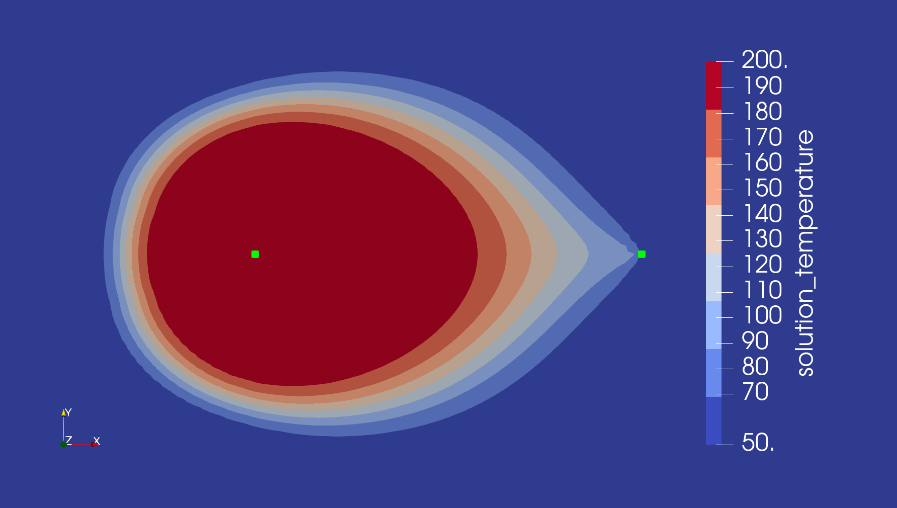
Figure 2: Aquifer temperature after injection of heated aquifer-brine into the system. The green dots show the injection and production borehole positions.
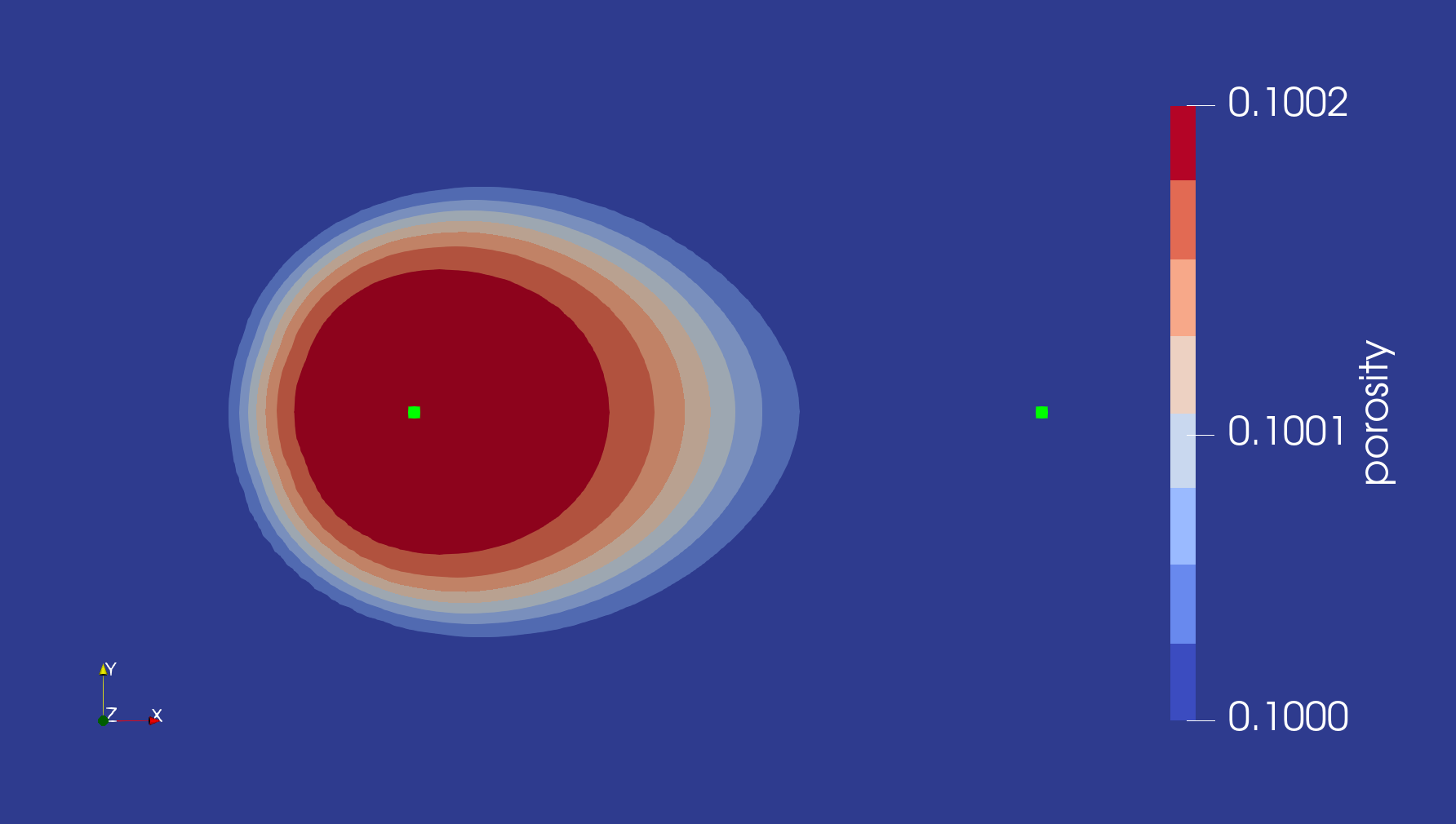
Figure 3: Aquifer porosity after injection of heated aquifer-brine into the system that causes dissolution of the aquifer quartz. The green dots show the injection and production borehole positions.
Comparison with QuartzUnlike
A very similar set of simulations, aquifer_un_quartz_geochemistry.i and exchanger_un_quartz.i may be found in the same directory. Instead of QuartzLike, these use the QuartzUnlike mineral, which precipitates upon heating rather than cooling. It is expected that the hot-fluid injection will have little impact upon the aquifer structure, but that lots of QuartzUnlike will precipitate in the heat exchanger as it heats the produced reservoir fluid. Indeed, the following figure shows this occurs:
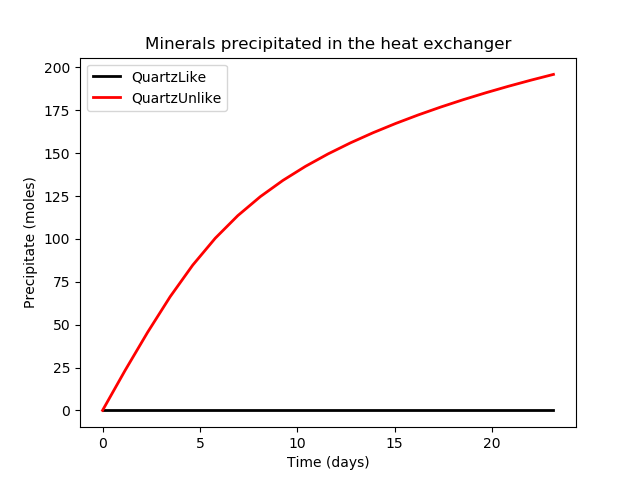
Figure 4: Minerals precipitated in the heat exchanger for the QuartzLike and QuartzUnlike cases. There are no QuartzLike precipitates because it becomes more soluble as it is heated, in contrast to the QuartzUnlike mineral.
(modules/combined/examples/geochem-porous_flow/geotes_2D/small_database.json)
{
  "Header": {
    "title": "Very small MOOSE thermodynamic database",
    "original": "moose/modules/geochemistry/python/original_dbs/gwb_llnl.dat",
    "date": "09:14 18-08-2020",
    "original format": "gwb",
    "activity model": "debye-huckel",
    "fugacity model": "tsonopoulos",
    "logk model": "fourth-order",
    "logk model (functional form)": "a0 + a1 T + a2 T^2 + a3 T^3 + a4 T^4",
    "temperatures": [
      0.0,
      25.0,
      60.0,
      100.0,
      150.0,
      200.0,
      250.0,
      300.0
    ],
    "pressures": [
      1.0134,
      1.0134,
      1.0134,
      1.0134,
      4.76,
      15.549,
      39.776,
      85.927
    ],
    "adh": [
      0.4913,
      0.5092,
      0.545,
      0.5998,
      0.6898,
      0.8099,
      0.9785,
      1.2555
    ],
    "bdh": [
      0.3247,
      0.3283,
      0.3343,
      0.3422,
      0.3533,
      0.3655,
      0.3792,
      0.3965
    ],
    "bdot": [
      0.0174,
      0.041,
      0.044,
      0.046,
      0.047,
      0.047,
      0.034,
      0.0
    ],
    "neutral species": {
      "co2": {
        "a": [
          0.1224,
          0.1127,
          0.09341,
          0.08018,
          0.08427,
          0.09892,
          0.1371,
          0.1967
        ],
        "b": [
          -0.004679,
          -0.01049,
          -0.0036,
          -0.001503,
          -0.01184,
          -0.0104,
          -0.007086,
          -0.01809
        ],
        "c": [
          -0.0004114,
          0.001545,
          9.609e-05,
          0.0005009,
          0.003118,
          0.001386,
          -0.002887,
          -0.002497
        ],
        "d": [
          0.0,
          0.0,
          0.0,
          0.0,
          0.0,
          0.0,
          0.0,
          0.0
        ]
      },
      "h2o": {
        "a": [
          1.4203,
          1.45397,
          1.5012,
          1.5551,
          1.6225,
          1.6899,
          1.7573,
          1.8247
        ],
        "note": "Missing array values in original database have been filled using a linear fit. Original values are [500.0000, -.0005362, 500.0000, -.0007132, -.0008312, 500.0000, 500.0000, 500.0000]",
        "b": [
          0.0177,
          0.022357,
          0.0289,
          0.036478,
          0.045891,
          0.0553,
          0.0647,
          0.0741
        ],
        "c": [
          0.0103,
          0.0093804,
          0.008,
          0.0064366,
          0.0045221,
          0.0026,
          0.0006,
          -0.0013
        ],
        "d": [
          -0.0005,
          -0.0005362,
          -0.0006,
          -0.0007132,
          -0.0008312,
          -0.0009,
          -0.0011,
          -0.0012
        ]
      }
    }
  },
  "elements": {
    "Cl": {
      "name": "Chlorine",
      "molecular weight": 35.453
    },
    "H": {
      "name": "Hydrogen",
      "molecular weight": 1.0079
    },
    "Na": {
      "name": "Sodium",
      "molecular weight": 22.9898
    },
    "O": {
      "name": "Oxygen",
      "molecular weight": 15.9994
    },
    "Si": {
      "name": "Silicon",
      "molecular weight": 28.085
    }
  },
  "basis species": {
    "H2O": {
      "elements": {
        "H": 2.0,
        "O": 1.0
      },
      "radius": 0.0,
      "charge": 0.0,
      "molecular weight": 18.0152
    },
    "Cl-": {
      "elements": {
        "Cl": 1.0
      },
      "radius": 3.0,
      "charge": -1.0,
      "molecular weight": 35.453
    },
    "Na+": {
      "elements": {
        "Na": 1.0
      },
      "radius": 4.0,
      "charge": 1.0,
      "molecular weight": 22.9898
    },
    "SiO2(aq)": {
      "elements": {
        "O": 2.0,
        "Si": 1.0
      },
      "radius": -0.5,
      "charge": 0.0,
      "molecular weight": 60.0843
    }
  },
  "secondary species": {
    "NaCl": {
      "species": {
        "Na+": 1.0,
        "Cl-": 1.0
      },
      "charge": 0.0,
      "radius": 4.0,
      "molecular weight": 58.4428,
      "logk": [
        1.855,
        1.5994,
        1.2945,
        0.9856,
        0.635,
        0.2935,
        -0.0407,
        -0.3487
      ],
      "note": "Missing array values in original database have been filled using a fourth-order fit. Original values are [1.8550, 1.5994, 1.2945, .9856, .6350, .2935, 500.0000, 500.0000]"
    }
  },
  "free electron": {
    "e-": {
      "species": {
        "H2O": 0.5,
        "O2(g)": -0.25,
        "H+": -1.0
      },
      "charge": -1.0,
      "radius": 0.0,
      "molecular weight": 0.0,
      "logk": [
        22.76135,
        20.7757,
        18.513025,
        16.4658,
        14.473225,
        12.92125,
        11.68165,
        10.67105
      ]
    }
  },
  "mineral species": {
    "QuartzLike": {
      "species": {
        "SiO2(aq)": 1.0
      },
      "molar volume": 22.688,
      "molecular weight": 60.0843,
      "logk": [-5.0, -4.0, -3.0, -2.0, -1.0, 0.0, 1.0, 2.0]
    },
    "QuartzUnlike": {
      "species": {
        "SiO2(aq)": 1.0
      },
      "molar volume": 22.688,
      "molecular weight": 60.0843,
      "logk": [-1.0, -2.0, -3.0, -4.0, -5.0, -6.0, -7.0, -8.0]
    }
  }
}
(modules/combined/examples/geochem-porous_flow/geotes_2D/aquifer_equilibrium.i)
# Finds the equilibrium free molality of SiO2(aq) when in contact with QuartzLike at 50degC
[UserObjects]
  [definition]
    type = GeochemicalModelDefinition
    database_file = "small_database.json"
    basis_species = "H2O SiO2(aq) Na+ Cl-"
    equilibrium_minerals = "QuartzLike"
  []
[]

[TimeIndependentReactionSolver]
  model_definition = definition
  geochemistry_reactor_name = reactor
  charge_balance_species = "Cl-"
  swap_out_of_basis = "SiO2(aq)"
  swap_into_basis = QuartzLike
  constraint_species = "H2O              Na+              Cl-              QuartzLike"
  constraint_value = "  1.0              0.1              0.1              396.685" # amount of QuartzLike is unimportant (provided it is positive).  396.685 is used simply because the other geotes_2D input files use this amount
  constraint_meaning = "kg_solvent_water bulk_composition bulk_composition free_mineral"
  constraint_unit = "   kg               moles            moles            moles"
  temperature = 50.0
  ramp_max_ionic_strength_initial = 0 # max_ionic_strength in such a simple problem does not need ramping
  add_aux_pH = false # there is no H+ in this system
  precision = 12
[]

[Postprocessors]
  [free_moles_SiO2]
    type = PointValue
    point = '0 0 0'
    variable = 'molal_SiO2(aq)'
  []
[]

[Outputs]
  csv = true
[]
(modules/combined/examples/geochem-porous_flow/geotes_2D/aquifer_geochemistry.i)
# Simulates geochemistry in the aquifer.  This input file may be run in standalone fashion but it does not do anything of interest.  To simulate something interesting, run the porous_flow.i simulation which couples to this input file using MultiApps.
# This file receives pf_rate_H2O, pf_rate_Na, pf_rate_Cl, pf_rate_SiO2 and temperature as AuxVariables from porous_flow.i.
# The pf_rate quantities are kg/s changes of fluid-component mass at each node, but the geochemistry module expects rates-of-changes of moles at every node.  Secondly, since this input file considers just 1 litre of aqueous solution at every node, the nodal_void_volume is used to convert pf_rate_* into rate_*_per_1l, which is measured in mol/s/1_litre_of_aqueous_solution.
# This file sends massfrac_Na, massfrac_Cl and massfrac_SiO2 to porous_flow.i.  These are computed from the corresponding transported_* quantities.
[Mesh]
  [gen]
    type = GeneratedMeshGenerator
    dim = 2
    nx = 14 # for better resolution, use 56 or 112
    ny = 8  # for better resolution, use 32 or 64
    xmin = -70
    xmax = 70
    ymin = -40
    ymax = 40
  []
[]

[GlobalParams]
  point = '0 0 0'
  reactor = reactor
[]

[SpatialReactionSolver]
  model_definition = definition
  geochemistry_reactor_name = reactor
  charge_balance_species = "Cl-"
  constraint_species = "H2O              Na+              Cl-              SiO2(aq)"
# ASSUME that 1 litre of solution contains:
  constraint_value = "  1.0              0.1              0.1              0.000555052386"
  constraint_meaning = "kg_solvent_water bulk_composition bulk_composition free_concentration"
  constraint_unit = "   kg               moles            moles            molal"
  initial_temperature = 50.0
  kinetic_species_name = QuartzLike
# Per 1 litre (1000cm^3) of aqueous solution (1kg of solvent water), there is 9000cm^3 of QuartzLike, which means the initial porosity is 0.1.
  kinetic_species_initial_value = 9000
  kinetic_species_unit = cm3
  temperature = temperature
  source_species_names = 'H2O    Na+   Cl-   SiO2(aq)'
  source_species_rates = 'rate_H2O_per_1l rate_Na_per_1l rate_Cl_per_1l rate_SiO2_per_1l'
  ramp_max_ionic_strength_initial = 0 # max_ionic_strength in such a simple problem does not need ramping
  add_aux_pH = false # there is no H+ in this system
  evaluate_kinetic_rates_always = true # implicit time-marching used for stability
  execute_console_output_on = ''
[]

[UserObjects]
  [rate_quartz]
    type = GeochemistryKineticRate
    kinetic_species_name = QuartzLike
    intrinsic_rate_constant = 1.0E-2
    multiply_by_mass = true
    area_quantity = 1
    activation_energy = 72800.0
  []
  [definition]
    type = GeochemicalModelDefinition
    database_file = "small_database.json"
    basis_species = "H2O SiO2(aq) Na+ Cl-"
    kinetic_minerals = "QuartzLike"
    kinetic_rate_descriptions = "rate_quartz"
  []
  [nodal_void_volume_uo]
    type = NodalVoidVolume
    porosity = porosity
    execute_on = 'initial timestep_end' # "initial" means this is evaluated properly for the first timestep
  []
[]


[Executioner]
  type = Transient
  dt = 1E5
  end_time = 7.76E6 # 90 days
[]

[AuxVariables]
  [temperature]
    initial_condition = 50.0
  []
  [porosity]
    initial_condition = 0.1
  []
  [nodal_void_volume]
  []
  [pf_rate_H2O] # change in H2O mass (kg/s) at each node provided by the porous-flow simulation
  []
  [pf_rate_Na] # change in H2O mass (kg/s) at each node provided by the porous-flow simulation
  []
  [pf_rate_Cl] # change in H2O mass (kg/s) at each node provided by the porous-flow simulation
  []
  [pf_rate_SiO2] # change in H2O mass (kg/s) at each node provided by the porous-flow simulation
  []
  [rate_H2O_per_1l] # rate per 1 litre of aqueous solution that we consider at each node
  []
  [rate_Na_per_1l]
  []
  [rate_Cl_per_1l]
  []
  [rate_SiO2_per_1l]
  []
  [transported_H2O]
  []
  [transported_Na]
  []
  [transported_Cl]
  []
  [transported_SiO2]
  []
  [transported_mass]
  []
  [massfrac_Na]
  []
  [massfrac_Cl]
  []
  [massfrac_SiO2]
  []
  [massfrac_H2O]
  []
[]
[AuxKernels]
  [porosity]
    type = ParsedAux
    coupled_variables = free_cm3_QuartzLike
    expression = '1000.0 / (1000.0 + free_cm3_QuartzLike)'
    variable = porosity
    execute_on = 'timestep_end'
  []
  [nodal_void_volume_auxk]
    type = NodalVoidVolumeAux
    variable = nodal_void_volume
    nodal_void_volume_uo = nodal_void_volume_uo
    execute_on = 'initial timestep_end' # "initial" to ensure it is properly evaluated for the first timestep
  []
  [rate_H2O_per_1l_auxk]
    type = ParsedAux
    coupled_variables = 'pf_rate_H2O nodal_void_volume'
    variable = rate_H2O_per_1l
# pf_rate = change in kg at every node
# pf_rate * 1000 / molar_mass_in_g_per_mole = change in moles at every node
# pf_rate * 1000 / molar_mass / (nodal_void_volume_in_m^3 * 1000) = change in moles per litre of aqueous solution
    expression = 'pf_rate_H2O / 18.0152 / nodal_void_volume'
    execute_on = 'timestep_begin'
  []
  [rate_Na_per_1l]
    type = ParsedAux
    coupled_variables = 'pf_rate_Na nodal_void_volume'
    variable = rate_Na_per_1l
    expression = 'pf_rate_Na / 22.9898 / nodal_void_volume'
    execute_on = 'timestep_begin'
  []
  [rate_Cl_per_1l]
    type = ParsedAux
    coupled_variables = 'pf_rate_Cl nodal_void_volume'
    variable = rate_Cl_per_1l
    expression = 'pf_rate_Cl / 35.453 / nodal_void_volume'
    execute_on = 'timestep_begin'
  []
  [rate_SiO2_per_1l]
    type = ParsedAux
    coupled_variables = 'pf_rate_SiO2 nodal_void_volume'
    variable = rate_SiO2_per_1l
    expression = 'pf_rate_SiO2 / 60.0843 / nodal_void_volume'
    execute_on = 'timestep_begin'
  []
  [transported_H2O_auxk]
    type = GeochemistryQuantityAux
    variable = transported_H2O
    species = H2O
    quantity = transported_moles_in_original_basis
    execute_on = 'timestep_end'
  []
  [transported_Na]
    type = GeochemistryQuantityAux
    variable = transported_Na
    species = Na+
    quantity = transported_moles_in_original_basis
    execute_on = 'timestep_end'
  []
  [transported_Cl]
    type = GeochemistryQuantityAux
    variable = transported_Cl
    species = Cl-
    quantity = transported_moles_in_original_basis
    execute_on = 'timestep_end'
  []
  [transported_SiO2]
    type = GeochemistryQuantityAux
    variable = transported_SiO2
    species = 'SiO2(aq)'
    quantity = transported_moles_in_original_basis
    execute_on = 'timestep_end'
  []
  [transported_mass_auxk]
    type = ParsedAux
    coupled_variables = 'transported_H2O transported_Na transported_Cl transported_SiO2'
    variable = transported_mass
    expression = 'transported_H2O * 18.0152 + transported_Na * 22.9898 + transported_Cl * 35.453 + transported_SiO2 * 60.0843'
    execute_on = 'timestep_end'
  []
  [massfrac_H2O]
    type = ParsedAux
    coupled_variables = 'transported_H2O transported_mass'
    variable = massfrac_H2O
    expression = 'transported_H2O * 18.0152 / transported_mass'
    execute_on = 'timestep_end'
  []
  [massfrac_Na]
    type = ParsedAux
    coupled_variables = 'transported_Na transported_mass'
    variable = massfrac_Na
    expression = 'transported_Na * 22.9898 / transported_mass'
    execute_on = 'timestep_end'
  []
  [massfrac_Cl]
    type = ParsedAux
    coupled_variables = 'transported_Cl transported_mass'
    variable = massfrac_Cl
    expression = 'transported_Cl * 35.453 / transported_mass'
    execute_on = 'timestep_end'
  []
  [massfrac_SiO2]
    type = ParsedAux
    coupled_variables = 'transported_SiO2 transported_mass'
    variable = massfrac_SiO2
    expression = 'transported_SiO2 * 60.0843 / transported_mass'
    execute_on = 'timestep_end'
  []
[]
[Postprocessors]
  [cm3_quartz]
    type = PointValue
    variable = free_cm3_QuartzLike
  []
  [porosity]
    type = PointValue
    variable = porosity
  []
  [solution_temperature]
    type = PointValue
    variable = solution_temperature
  []
  [massfrac_H2O]
    type = PointValue
    variable = massfrac_H2O
  []
  [massfrac_Na]
    type = PointValue
    variable = massfrac_Na
  []
  [massfrac_Cl]
    type = PointValue
    variable = massfrac_Cl
  []
  [massfrac_SiO2]
    type = PointValue
    variable = massfrac_SiO2
  []
[]

[Outputs]
  exodus = true
  csv = true
[]
(modules/combined/examples/geochem-porous_flow/geotes_2D/porous_flow.i)
# PorousFlow simulation of injection and production in a 2D aquifer
# Much of this file is standard porous-flow stuff.  The unusual aspects are:
# - transfer of the rates of changes of each species (kg/s) to the aquifer_geochemistry.i simulation.  This is achieved by saving these changes from the PorousFlowMassTimeDerivative residuals
# - transfer of the temperature field to the aquifer_geochemistry.i simulation
# Interesting behaviour can be simulated by this file without its "parent" simulation, exchanger.i.  exchanger.i provides mass-fractions injected via the injection_rate_massfrac_* variables, but since these are more-or-less constant throughout the duration of the exchanger.i simulation, the initial_conditions specified below may be used.  Similar, exchanger.i provides injection_temperature, but that is also constant.

injection_rate = -1.0 # kg/s/m, negative because injection as a source
production_rate = 1.0 # kg/s/m
[Mesh]
  [gen]
    type = GeneratedMeshGenerator
    dim = 2
    nx = 14 # for better resolution, use 56 or 112
    ny = 8  # for better resolution, use 32 or 64
    xmin = -70
    xmax = 70
    ymin = -40
    ymax = 40
  []
  [injection_node]
    input = gen
    type = ExtraNodesetGenerator
    new_boundary = injection_node
    coord = '-30 0 0'
  []
[]

[GlobalParams]
  PorousFlowDictator = dictator
  gravity = '0 0 0'
[]

[Variables]
  [f0]
    initial_condition = 0.002285946
  []
  [f1]
    initial_condition = 0.0035252
  []
  [f2]
    initial_condition = 1.3741E-05
  []
  [porepressure]
    initial_condition = 2E6
  []
  [temperature]
    initial_condition = 50
    scaling = 1E-6 # fluid enthalpy is roughly 1E6
  []
[]

[BCs]
  [injection_temperature]
    type = MatchedValueBC
    variable = temperature
    v = injection_temperature
    boundary = injection_node
  []
[]

[DiracKernels]
  [inject_Na]
    type = PorousFlowPolyLineSink
    SumQuantityUO = injected_mass
    fluxes = ${injection_rate}
    p_or_t_vals = 0.0
    line_length = 1.0
    multiplying_var = injection_rate_massfrac_Na
    point_file = injection.bh
    variable = f0
  []
  [inject_Cl]
    type = PorousFlowPolyLineSink
    SumQuantityUO = injected_mass
    fluxes = ${injection_rate}
    p_or_t_vals = 0.0
    line_length = 1.0
    multiplying_var = injection_rate_massfrac_Cl
    point_file = injection.bh
    variable = f1
  []
  [inject_SiO2]
    type = PorousFlowPolyLineSink
    SumQuantityUO = injected_mass
    fluxes = ${injection_rate}
    p_or_t_vals = 0.0
    line_length = 1.0
    multiplying_var = injection_rate_massfrac_SiO2
    point_file = injection.bh
    variable = f2
  []
  [inject_H2O]
    type = PorousFlowPolyLineSink
    SumQuantityUO = injected_mass
    fluxes = ${injection_rate}
    p_or_t_vals = 0.0
    line_length = 1.0
    multiplying_var = injection_rate_massfrac_H2O
    point_file = injection.bh
    variable = porepressure
  []

  [produce_Na]
    type = PorousFlowPolyLineSink
    SumQuantityUO = produced_mass_Na
    fluxes = ${production_rate}
    p_or_t_vals = 0.0
    line_length = 1.0
    mass_fraction_component = 0
    point_file = production.bh
    variable = f0
  []
  [produce_Cl]
    type = PorousFlowPolyLineSink
    SumQuantityUO = produced_mass_Cl
    fluxes = ${production_rate}
    p_or_t_vals = 0.0
    line_length = 1.0
    mass_fraction_component = 1
    point_file = production.bh
    variable = f1
  []
  [produce_SiO2]
    type = PorousFlowPolyLineSink
    SumQuantityUO = produced_mass_SiO2
    fluxes = ${production_rate}
    p_or_t_vals = 0.0
    line_length = 1.0
    mass_fraction_component = 2
    point_file = production.bh
    variable = f2
  []
  [produce_H2O]
    type = PorousFlowPolyLineSink
    SumQuantityUO = produced_mass_H2O
    fluxes = ${production_rate}
    p_or_t_vals = 0.0
    line_length = 1.0
    mass_fraction_component = 3
    point_file = production.bh
    variable = porepressure
  []
  [produce_heat]
    type = PorousFlowPolyLineSink
    SumQuantityUO = produced_heat
    fluxes = ${production_rate}
    p_or_t_vals = 0.0
    line_length = 1.0
    use_enthalpy = true
    point_file = production.bh
    variable = temperature
  []
[]

[UserObjects]
  [injected_mass]
    type = PorousFlowSumQuantity
  []
  [produced_mass_Na]
    type = PorousFlowSumQuantity
  []
  [produced_mass_Cl]
    type = PorousFlowSumQuantity
  []
  [produced_mass_SiO2]
    type = PorousFlowSumQuantity
  []
  [produced_mass_H2O]
    type = PorousFlowSumQuantity
  []
  [produced_heat]
    type = PorousFlowSumQuantity
  []
[]

[Postprocessors]
  [dt]
    type = TimestepSize
    execute_on = TIMESTEP_BEGIN
  []
  [tot_kg_injected_this_timestep]
    type = PorousFlowPlotQuantity
    uo = injected_mass
  []
  [kg_Na_produced_this_timestep]
    type = PorousFlowPlotQuantity
    uo = produced_mass_Na
  []
  [kg_Cl_produced_this_timestep]
    type = PorousFlowPlotQuantity
    uo = produced_mass_Cl
  []
  [kg_SiO2_produced_this_timestep]
    type = PorousFlowPlotQuantity
    uo = produced_mass_SiO2
  []
  [kg_H2O_produced_this_timestep]
    type = PorousFlowPlotQuantity
    uo = produced_mass_H2O
  []
  [mole_rate_Na_produced]
    type = FunctionValuePostprocessor
    function = moles_Na
    indirect_dependencies = 'kg_Na_produced_this_timestep dt'
  []
  [mole_rate_Cl_produced]
    type = FunctionValuePostprocessor
    function = moles_Cl
    indirect_dependencies = 'kg_Cl_produced_this_timestep dt'
  []
  [mole_rate_SiO2_produced]
    type = FunctionValuePostprocessor
    function = moles_SiO2
    indirect_dependencies = 'kg_SiO2_produced_this_timestep dt'
  []
  [mole_rate_H2O_produced]
    type = FunctionValuePostprocessor
    function = moles_H2O
    indirect_dependencies = 'kg_H2O_produced_this_timestep dt'
  []
  [heat_joules_extracted_this_timestep]
    type = PorousFlowPlotQuantity
    uo = produced_heat
  []
  [production_temperature]
    type = PointValue
    point = '30 0 0'
    variable = temperature
  []
[]

[Functions]
  [moles_Na]
    type = ParsedFunction
    symbol_names = 'kg_Na dt'
    symbol_values = 'kg_Na_produced_this_timestep dt'
    expression = 'kg_Na * 1000 / 22.9898 / dt'
  []
  [moles_Cl]
    type = ParsedFunction
    symbol_names = 'kg_Cl dt'
    symbol_values = 'kg_Cl_produced_this_timestep dt'
    expression = 'kg_Cl * 1000 / 35.453 / dt'
  []
  [moles_SiO2]
    type = ParsedFunction
    symbol_names = 'kg_SiO2 dt'
    symbol_values = 'kg_SiO2_produced_this_timestep dt'
    expression = 'kg_SiO2 * 1000 / 60.0843 / dt'
  []
  [moles_H2O]
    type = ParsedFunction
    symbol_names = 'kg_H2O dt'
    symbol_values = 'kg_H2O_produced_this_timestep dt'
    expression = 'kg_H2O * 1000 / 18.0152 / dt'
  []
[]

[FluidProperties]
  [the_simple_fluid]
    type = SimpleFluidProperties
    thermal_expansion = 0
    bulk_modulus = 2E9
    viscosity = 1E-3
    density0 = 1000
    cv = 4000.0
    cp = 4000.0
  []
[]

[PorousFlowFullySaturated]
  coupling_type = ThermoHydro
  porepressure = porepressure
  temperature = temperature
  mass_fraction_vars = 'f0 f1 f2'
  save_component_rate_in = 'rate_Na rate_Cl rate_SiO2 rate_H2O' # change in kg at every node / dt
  fp = the_simple_fluid
  temperature_unit = Celsius
[]

[AuxVariables]
  [injection_temperature]
    initial_condition = 200
  []
  [injection_rate_massfrac_Na]
    initial_condition = 0.002285946
  []
  [injection_rate_massfrac_Cl]
    initial_condition = 0.0035252
  []
  [injection_rate_massfrac_SiO2]
    initial_condition = 1.3741E-05
  []
  [injection_rate_massfrac_H2O]
    initial_condition = 0.994175112
  []
  [rate_H2O]
  []
  [rate_Na]
  []
  [rate_Cl]
  []
  [rate_SiO2]
  []
[]

[Materials]
  [porosity]
    type = PorousFlowPorosityConst # this simulation has no porosity changes from dissolution
    porosity = 0.1
  []
  [permeability]
    type = PorousFlowPermeabilityConst
    permeability = '1E-12 0 0   0 1E-12 0   0 0 1E-12'
  []
  [thermal_conductivity]
    type = PorousFlowThermalConductivityIdeal
    dry_thermal_conductivity = '0 0 0  0 0 0  0 0 0'
  []
  [rock_heat]
    type = PorousFlowMatrixInternalEnergy
    density = 2500.0
    specific_heat_capacity = 1200.0
  []
[]

[Preconditioning]
  active = typically_efficient
  [typically_efficient]
    type = SMP
    full = true
    petsc_options_iname = '-pc_type -pc_hypre_type'
    petsc_options_value = ' hypre    boomeramg'
  []
  [strong]
    type = SMP
    full = true
    petsc_options = '-ksp_diagonal_scale -ksp_diagonal_scale_fix'
    petsc_options_iname = '-pc_type -sub_pc_type -sub_pc_factor_shift_type -pc_asm_overlap'
    petsc_options_value = ' asm      ilu           NONZERO                   2'
  []
  [probably_too_strong]
    type = SMP
    full = true
    petsc_options_iname = '-pc_type -pc_factor_mat_solver_package'
    petsc_options_value = ' lu       mumps'
  []
[]

[Executioner]
  type = Transient
  solve_type = Newton
  end_time = 7.76E6 # 90 days
  dt = 1E5
[]

[Outputs]
  exodus = true
[]

[MultiApps]
  [react]
    type = TransientMultiApp
    input_files = aquifer_geochemistry.i
    clone_master_mesh = true
    execute_on = 'timestep_end'
  []
[]

[Transfers]
  [changes_due_to_flow]
    type = MultiAppCopyTransfer
    source_variable = 'rate_H2O rate_Na rate_Cl rate_SiO2 temperature'
    variable = 'pf_rate_H2O pf_rate_Na pf_rate_Cl pf_rate_SiO2 temperature'
    to_multi_app = react
  []
  [massfrac_from_geochem]
    type = MultiAppCopyTransfer
    source_variable = 'massfrac_Na massfrac_Cl massfrac_SiO2'
    variable = 'f0 f1 f2'
    from_multi_app = react
  []
[]
(modules/combined/examples/geochem-porous_flow/geotes_2D/production.bh)
1.0 30 0 0
(modules/combined/examples/geochem-porous_flow/geotes_2D/porous_flow.i)
# PorousFlow simulation of injection and production in a 2D aquifer
# Much of this file is standard porous-flow stuff.  The unusual aspects are:
# - transfer of the rates of changes of each species (kg/s) to the aquifer_geochemistry.i simulation.  This is achieved by saving these changes from the PorousFlowMassTimeDerivative residuals
# - transfer of the temperature field to the aquifer_geochemistry.i simulation
# Interesting behaviour can be simulated by this file without its "parent" simulation, exchanger.i.  exchanger.i provides mass-fractions injected via the injection_rate_massfrac_* variables, but since these are more-or-less constant throughout the duration of the exchanger.i simulation, the initial_conditions specified below may be used.  Similar, exchanger.i provides injection_temperature, but that is also constant.

injection_rate = -1.0 # kg/s/m, negative because injection as a source
production_rate = 1.0 # kg/s/m
[Mesh]
  [gen]
    type = GeneratedMeshGenerator
    dim = 2
    nx = 14 # for better resolution, use 56 or 112
    ny = 8  # for better resolution, use 32 or 64
    xmin = -70
    xmax = 70
    ymin = -40
    ymax = 40
  []
  [injection_node]
    input = gen
    type = ExtraNodesetGenerator
    new_boundary = injection_node
    coord = '-30 0 0'
  []
[]

[GlobalParams]
  PorousFlowDictator = dictator
  gravity = '0 0 0'
[]

[Variables]
  [f0]
    initial_condition = 0.002285946
  []
  [f1]
    initial_condition = 0.0035252
  []
  [f2]
    initial_condition = 1.3741E-05
  []
  [porepressure]
    initial_condition = 2E6
  []
  [temperature]
    initial_condition = 50
    scaling = 1E-6 # fluid enthalpy is roughly 1E6
  []
[]

[BCs]
  [injection_temperature]
    type = MatchedValueBC
    variable = temperature
    v = injection_temperature
    boundary = injection_node
  []
[]

[DiracKernels]
  [inject_Na]
    type = PorousFlowPolyLineSink
    SumQuantityUO = injected_mass
    fluxes = ${injection_rate}
    p_or_t_vals = 0.0
    line_length = 1.0
    multiplying_var = injection_rate_massfrac_Na
    point_file = injection.bh
    variable = f0
  []
  [inject_Cl]
    type = PorousFlowPolyLineSink
    SumQuantityUO = injected_mass
    fluxes = ${injection_rate}
    p_or_t_vals = 0.0
    line_length = 1.0
    multiplying_var = injection_rate_massfrac_Cl
    point_file = injection.bh
    variable = f1
  []
  [inject_SiO2]
    type = PorousFlowPolyLineSink
    SumQuantityUO = injected_mass
    fluxes = ${injection_rate}
    p_or_t_vals = 0.0
    line_length = 1.0
    multiplying_var = injection_rate_massfrac_SiO2
    point_file = injection.bh
    variable = f2
  []
  [inject_H2O]
    type = PorousFlowPolyLineSink
    SumQuantityUO = injected_mass
    fluxes = ${injection_rate}
    p_or_t_vals = 0.0
    line_length = 1.0
    multiplying_var = injection_rate_massfrac_H2O
    point_file = injection.bh
    variable = porepressure
  []

  [produce_Na]
    type = PorousFlowPolyLineSink
    SumQuantityUO = produced_mass_Na
    fluxes = ${production_rate}
    p_or_t_vals = 0.0
    line_length = 1.0
    mass_fraction_component = 0
    point_file = production.bh
    variable = f0
  []
  [produce_Cl]
    type = PorousFlowPolyLineSink
    SumQuantityUO = produced_mass_Cl
    fluxes = ${production_rate}
    p_or_t_vals = 0.0
    line_length = 1.0
    mass_fraction_component = 1
    point_file = production.bh
    variable = f1
  []
  [produce_SiO2]
    type = PorousFlowPolyLineSink
    SumQuantityUO = produced_mass_SiO2
    fluxes = ${production_rate}
    p_or_t_vals = 0.0
    line_length = 1.0
    mass_fraction_component = 2
    point_file = production.bh
    variable = f2
  []
  [produce_H2O]
    type = PorousFlowPolyLineSink
    SumQuantityUO = produced_mass_H2O
    fluxes = ${production_rate}
    p_or_t_vals = 0.0
    line_length = 1.0
    mass_fraction_component = 3
    point_file = production.bh
    variable = porepressure
  []
  [produce_heat]
    type = PorousFlowPolyLineSink
    SumQuantityUO = produced_heat
    fluxes = ${production_rate}
    p_or_t_vals = 0.0
    line_length = 1.0
    use_enthalpy = true
    point_file = production.bh
    variable = temperature
  []
[]

[UserObjects]
  [injected_mass]
    type = PorousFlowSumQuantity
  []
  [produced_mass_Na]
    type = PorousFlowSumQuantity
  []
  [produced_mass_Cl]
    type = PorousFlowSumQuantity
  []
  [produced_mass_SiO2]
    type = PorousFlowSumQuantity
  []
  [produced_mass_H2O]
    type = PorousFlowSumQuantity
  []
  [produced_heat]
    type = PorousFlowSumQuantity
  []
[]

[Postprocessors]
  [dt]
    type = TimestepSize
    execute_on = TIMESTEP_BEGIN
  []
  [tot_kg_injected_this_timestep]
    type = PorousFlowPlotQuantity
    uo = injected_mass
  []
  [kg_Na_produced_this_timestep]
    type = PorousFlowPlotQuantity
    uo = produced_mass_Na
  []
  [kg_Cl_produced_this_timestep]
    type = PorousFlowPlotQuantity
    uo = produced_mass_Cl
  []
  [kg_SiO2_produced_this_timestep]
    type = PorousFlowPlotQuantity
    uo = produced_mass_SiO2
  []
  [kg_H2O_produced_this_timestep]
    type = PorousFlowPlotQuantity
    uo = produced_mass_H2O
  []
  [mole_rate_Na_produced]
    type = FunctionValuePostprocessor
    function = moles_Na
    indirect_dependencies = 'kg_Na_produced_this_timestep dt'
  []
  [mole_rate_Cl_produced]
    type = FunctionValuePostprocessor
    function = moles_Cl
    indirect_dependencies = 'kg_Cl_produced_this_timestep dt'
  []
  [mole_rate_SiO2_produced]
    type = FunctionValuePostprocessor
    function = moles_SiO2
    indirect_dependencies = 'kg_SiO2_produced_this_timestep dt'
  []
  [mole_rate_H2O_produced]
    type = FunctionValuePostprocessor
    function = moles_H2O
    indirect_dependencies = 'kg_H2O_produced_this_timestep dt'
  []
  [heat_joules_extracted_this_timestep]
    type = PorousFlowPlotQuantity
    uo = produced_heat
  []
  [production_temperature]
    type = PointValue
    point = '30 0 0'
    variable = temperature
  []
[]

[Functions]
  [moles_Na]
    type = ParsedFunction
    symbol_names = 'kg_Na dt'
    symbol_values = 'kg_Na_produced_this_timestep dt'
    expression = 'kg_Na * 1000 / 22.9898 / dt'
  []
  [moles_Cl]
    type = ParsedFunction
    symbol_names = 'kg_Cl dt'
    symbol_values = 'kg_Cl_produced_this_timestep dt'
    expression = 'kg_Cl * 1000 / 35.453 / dt'
  []
  [moles_SiO2]
    type = ParsedFunction
    symbol_names = 'kg_SiO2 dt'
    symbol_values = 'kg_SiO2_produced_this_timestep dt'
    expression = 'kg_SiO2 * 1000 / 60.0843 / dt'
  []
  [moles_H2O]
    type = ParsedFunction
    symbol_names = 'kg_H2O dt'
    symbol_values = 'kg_H2O_produced_this_timestep dt'
    expression = 'kg_H2O * 1000 / 18.0152 / dt'
  []
[]

[FluidProperties]
  [the_simple_fluid]
    type = SimpleFluidProperties
    thermal_expansion = 0
    bulk_modulus = 2E9
    viscosity = 1E-3
    density0 = 1000
    cv = 4000.0
    cp = 4000.0
  []
[]

[PorousFlowFullySaturated]
  coupling_type = ThermoHydro
  porepressure = porepressure
  temperature = temperature
  mass_fraction_vars = 'f0 f1 f2'
  save_component_rate_in = 'rate_Na rate_Cl rate_SiO2 rate_H2O' # change in kg at every node / dt
  fp = the_simple_fluid
  temperature_unit = Celsius
[]

[AuxVariables]
  [injection_temperature]
    initial_condition = 200
  []
  [injection_rate_massfrac_Na]
    initial_condition = 0.002285946
  []
  [injection_rate_massfrac_Cl]
    initial_condition = 0.0035252
  []
  [injection_rate_massfrac_SiO2]
    initial_condition = 1.3741E-05
  []
  [injection_rate_massfrac_H2O]
    initial_condition = 0.994175112
  []
  [rate_H2O]
  []
  [rate_Na]
  []
  [rate_Cl]
  []
  [rate_SiO2]
  []
[]

[Materials]
  [porosity]
    type = PorousFlowPorosityConst # this simulation has no porosity changes from dissolution
    porosity = 0.1
  []
  [permeability]
    type = PorousFlowPermeabilityConst
    permeability = '1E-12 0 0   0 1E-12 0   0 0 1E-12'
  []
  [thermal_conductivity]
    type = PorousFlowThermalConductivityIdeal
    dry_thermal_conductivity = '0 0 0  0 0 0  0 0 0'
  []
  [rock_heat]
    type = PorousFlowMatrixInternalEnergy
    density = 2500.0
    specific_heat_capacity = 1200.0
  []
[]

[Preconditioning]
  active = typically_efficient
  [typically_efficient]
    type = SMP
    full = true
    petsc_options_iname = '-pc_type -pc_hypre_type'
    petsc_options_value = ' hypre    boomeramg'
  []
  [strong]
    type = SMP
    full = true
    petsc_options = '-ksp_diagonal_scale -ksp_diagonal_scale_fix'
    petsc_options_iname = '-pc_type -sub_pc_type -sub_pc_factor_shift_type -pc_asm_overlap'
    petsc_options_value = ' asm      ilu           NONZERO                   2'
  []
  [probably_too_strong]
    type = SMP
    full = true
    petsc_options_iname = '-pc_type -pc_factor_mat_solver_package'
    petsc_options_value = ' lu       mumps'
  []
[]

[Executioner]
  type = Transient
  solve_type = Newton
  end_time = 7.76E6 # 90 days
  dt = 1E5
[]

[Outputs]
  exodus = true
[]

[MultiApps]
  [react]
    type = TransientMultiApp
    input_files = aquifer_geochemistry.i
    clone_master_mesh = true
    execute_on = 'timestep_end'
  []
[]

[Transfers]
  [changes_due_to_flow]
    type = MultiAppCopyTransfer
    source_variable = 'rate_H2O rate_Na rate_Cl rate_SiO2 temperature'
    variable = 'pf_rate_H2O pf_rate_Na pf_rate_Cl pf_rate_SiO2 temperature'
    to_multi_app = react
  []
  [massfrac_from_geochem]
    type = MultiAppCopyTransfer
    source_variable = 'massfrac_Na massfrac_Cl massfrac_SiO2'
    variable = 'f0 f1 f2'
    from_multi_app = react
  []
[]
(modules/combined/examples/geochem-porous_flow/geotes_2D/exchanger.i)
# Model of the heat-exchanger
# The input fluid to the heat exchanger is determined by AuxVariables called production_temperature, production_rate_Na, production_rate_Cl, production_rate_SiO2 and production_rate_H2O.  These come from Postprocessors in the porous-flow simulation that measure the fluid composition at the production well.
# Given the input fluid, the exchanger cools/heats the fluid, removing any precipitates, and injects fluid back to the porous-flow simulation at temperature output_temperature and composition given by massfrac_Na, etc.
# In the absence of data concerning Quartz precipitation rates in heat exchangers, do not treat Quartz as kinetic
[GlobalParams]
  point = '0 0 0'
  reactor = reactor
[]

[TimeDependentReactionSolver]
  model_definition = definition
  include_moose_solve = false
  geochemistry_reactor_name = reactor
  charge_balance_species = "Cl-"
  swap_out_of_basis = "SiO2(aq)"
  swap_into_basis = "QuartzLike"
  constraint_species = "H2O              Na+              Cl-              QuartzLike"
  constraint_value = "  1.0E-2           0.1E-2           0.1E-2           1E-10"
  constraint_meaning = "kg_solvent_water bulk_composition bulk_composition free_mineral"
  constraint_unit = "   kg               moles            moles            moles"
  initial_temperature = 50.0
  mode = 4
  temperature = 200
  cold_temperature = 40.0
  source_species_names = 'H2O    Na+   Cl-   SiO2(aq)'
  source_species_rates = 'production_rate_H2O production_rate_Na production_rate_Cl production_rate_SiO2'
  ramp_max_ionic_strength_initial = 0 # max_ionic_strength in such a simple problem does not need ramping
  add_aux_pH = false # there is no H+ in this system
  evaluate_kinetic_rates_always = true # implicit time-marching used for stability
  execute_console_output_on = '' # only CSV output used in this example
[]

[UserObjects]
  [definition]
    type = GeochemicalModelDefinition
    database_file = "small_database.json"
    basis_species = "H2O SiO2(aq) Na+ Cl-"
    equilibrium_minerals = "QuartzLike"
  []
[]

[Executioner]
  type = Transient
  dt = 1E5
  end_time = 2E6 #7.76E6 # 90 days
[]

[AuxVariables]
  [production_temperature]
    initial_condition = 50 # the production_T Transfer lags one timestep behind for some reason, so give this a reasonable initial condition
  []
  [transported_H2O]
  []
  [transported_Na]
  []
  [transported_Cl]
  []
  [transported_SiO2]
  []
  [transported_mass]
  []
  [massfrac_H2O]
  []
  [massfrac_Na]
  []
  [massfrac_Cl]
  []
  [massfrac_SiO2]
  []
  [dumped_quartz]
  []
  [production_rate_H2O]
    initial_condition = 5.518533e+01 # the production_H2O Transfer lags one timestep behind for some reason (when the porous_flow simulation has finished, it correctly computes mole_rate_H2O_produced, but the Transfer gets the mole_rate_H2O_produced from the previous timestep), so give this a reasonable initial condition, otherwise this will be zero at the start of the simulation!
  []
  [production_rate_Na]
    initial_condition = 9.943302e-02
  []
  [production_rate_Cl]
    initial_condition = 9.943302e-02
  []
  [production_rate_SiO2]
    initial_condition = 2.340931e-04
  []
[]
[AuxKernels]
  [transported_H2O_auxk]
    type = GeochemistryQuantityAux
    variable = transported_H2O
    species = H2O
    quantity = transported_moles_in_original_basis
  []
  [transported_Na]
    type = GeochemistryQuantityAux
    variable = transported_Na
    species = Na+
    quantity = transported_moles_in_original_basis
  []
  [transported_Cl]
    type = GeochemistryQuantityAux
    variable = transported_Cl
    species = Cl-
    quantity = transported_moles_in_original_basis
  []
  [transported_SiO2]
    type = GeochemistryQuantityAux
    variable = transported_SiO2
    species = 'SiO2(aq)'
    quantity = transported_moles_in_original_basis
  []
  [transported_mass_auxk]
    type = ParsedAux
    coupled_variables = 'transported_H2O transported_Na transported_Cl transported_SiO2'
    variable = transported_mass
    expression = 'transported_H2O * 18.0152 + transported_Na * 22.9898 + transported_Cl * 35.453 + transported_SiO2 * 60.0843'
  []
  [massfrac_H2O]
    type = ParsedAux
    coupled_variables = 'transported_mass transported_H2O'
    variable = massfrac_H2O
    expression = '18.0152 * transported_H2O / transported_mass'
  []
  [massfrac_Na]
    type = ParsedAux
    coupled_variables = 'transported_mass transported_Na'
    variable = massfrac_Na
    expression = '22.9898 * transported_Na / transported_mass'
  []
  [massfrac_Cl]
    type = ParsedAux
    coupled_variables = 'transported_mass transported_Cl'
    variable = massfrac_Cl
    expression = '35.453 * transported_Cl / transported_mass'
  []
  [massfrac_SiO2]
    type = ParsedAux
    coupled_variables = 'transported_mass transported_SiO2'
    variable = massfrac_SiO2
    expression = '60.0843 * transported_SiO2 / transported_mass'
  []
  [dumped_quartz]
    type = GeochemistryQuantityAux
    variable = dumped_quartz
    species = QuartzLike
    quantity = moles_dumped
  []
[]
[Postprocessors]
  [cumulative_moles_precipitated_quartz]
    type = PointValue
    variable = dumped_quartz
  []
  [production_temperature]
    type = PointValue
    variable = production_temperature
  []
  [mass_heated_this_timestep]
    type = PointValue
    variable = transported_mass
  []
[]
[Outputs]
  csv = true
[]

[MultiApps]
  [porous_flow_sim]
    type = TransientMultiApp
    input_files = porous_flow.i
    execute_on = 'timestep_end'
  []
[]

[Transfers]
  [injection_T]
    type = MultiAppNearestNodeTransfer
    direction = TO_MULTIAPP
    multi_app = porous_flow_sim
    fixed_meshes = true
    source_variable = 'solution_temperature'
    variable = 'injection_temperature'
  []
  [injection_Na]
    type = MultiAppNearestNodeTransfer
    direction = TO_MULTIAPP
    multi_app = porous_flow_sim
    fixed_meshes = true
    source_variable = 'massfrac_Na'
    variable = 'injection_rate_massfrac_Na'
  []
  [injection_Cl]
    type = MultiAppNearestNodeTransfer
    direction = TO_MULTIAPP
    multi_app = porous_flow_sim
    fixed_meshes = true
    source_variable = 'massfrac_Cl'
    variable = 'injection_rate_massfrac_Cl'
  []
  [injection_SiO2]
    type = MultiAppNearestNodeTransfer
    direction = TO_MULTIAPP
    multi_app = porous_flow_sim
    fixed_meshes = true
    source_variable = 'massfrac_SiO2'
    variable = 'injection_rate_massfrac_SiO2'
  []
  [injection_H2O]
    type = MultiAppNearestNodeTransfer
    direction = TO_MULTIAPP
    multi_app = porous_flow_sim
    fixed_meshes = true
    source_variable = 'massfrac_H2O'
    variable = 'injection_rate_massfrac_H2O'
  []

  [production_T]
    type = MultiAppPostprocessorInterpolationTransfer
    direction = FROM_MULTIAPP
    multi_app = porous_flow_sim
    postprocessor = production_temperature
    variable = production_temperature
  []
  [production_Na]
    type = MultiAppPostprocessorInterpolationTransfer
    direction = FROM_MULTIAPP
    multi_app = porous_flow_sim
    postprocessor = mole_rate_Na_produced
    variable = production_rate_Na
  []
  [production_Cl]
    type = MultiAppPostprocessorInterpolationTransfer
    direction = FROM_MULTIAPP
    multi_app = porous_flow_sim
    postprocessor = mole_rate_Cl_produced
    variable = production_rate_Cl
  []
  [production_SiO2]
    type = MultiAppPostprocessorInterpolationTransfer
    direction = FROM_MULTIAPP
    multi_app = porous_flow_sim
    postprocessor = mole_rate_SiO2_produced
    variable = production_rate_SiO2
  []
  [production_H2O]
    type = MultiAppPostprocessorInterpolationTransfer
    direction = FROM_MULTIAPP
    multi_app = porous_flow_sim
    postprocessor = mole_rate_H2O_produced
    variable = production_rate_H2O
  []
[]