Porous Flow Tutorial Page 13. More elaborate chemistry
A very simple chemical system was built in Page 07. The reader is encouraged to consult that page before moving to the more elaborate situation described here. This page:
does not use an
Actionto describe the Kernels, Materials, etc. This makes the input file quite long, but perhaps more easy to extend to multi-phase situations, different boundary conditions, etc. AnActioncould easily be used instead, by copying the chemistry from this tutorial to that on Page 07.builds a fully-saturated aqueous chemical system that could be used to describe dolomite precipitation and dissolution.
This page illustrates that it is possible to build quite complicated chemical systems within PorousFlow. However, geochemists will recognize these are still unrealistically simple, since they contain only a few species, the activity coefficients are all unity, the equilibrium constants are not easily temperature-dependent, etc. If you require state-of-the-art geochemical modelling capability, please use MOOSE's Geochemistry module.
The equilibrium system
The equilibrium system has:
5 primary species, which are H, HCO, Ca, Mg, Fe.
5 secondary species, which are CO(aq), CO, CaHCO, MgHCO, FeHCO.
The equations are Some of these equilibrium constants have been chosen rather arbitrarily.
The primary species are represented as PorousFlow variables:
[Variables<<<{"href": "../../syntax/Variables/index.html"}>>>]
  [h+]
  []
  [hco3-]
  []
  [ca2+]
  []
  [mg2+]
  []
  [fe2+]
  []
[]The equilibrium reactions are encoded into this Material:
  [equilibrium_massfrac]
    type = PorousFlowMassFractionAqueousEquilibriumChemistry
    mass_fraction_vars = 'h+ hco3- ca2+ mg2+ fe2+'
    num_reactions = 5
    equilibrium_constants = 'eqm_k0 eqm_k1 eqm_k2 eqm_k3 eqm_k4'
    primary_activity_coefficients = '1 1 1 1 1'
    secondary_activity_coefficients = '1 1 1 1 1'
    reactions = '1 1 0 0 0
                -1 1 0 0 0
                 0 1 1 0 0
                 0 1 0 1 0
                 0 1 0 0 1'
[]The kinetic system
This is with the following parameters:
molar volume 64365.0L(solution)/mol,
mineral density 2875.0kg(precipitate)/m(precipitate)
equilibrium constant ,
specific reactive surface area m/L,
kinetic rate constant mol/m/s,
activation energy J/mol,
the primary activity coefficients are all unity,
and the and exponents are also unity.
Some of these quantities have been chosen rather arbitrarily. This kinetic system is encoded in the input file as:
  [kinetic]
    type = PorousFlowAqueousPreDisChemistry
    primary_concentrations = 'h+ hco3- ca2+ mg2+ fe2+'
    num_reactions = 1
    equilibrium_constants = kinetic_k
    primary_activity_coefficients = '1 1 1 1 1'
    reactions = '-2 2 1 0.8 0.2'
    specific_reactive_surface_area = '1.2E-8'
    kinetic_rate_constant = '3E-4'
    activation_energy = '1.5e4'
    molar_volume = 64365.0
    gas_constant = 8.314
    reference_temperature = 298.15
[]Geometry
The model is just a 1D line, extending between and .
[Mesh<<<{"href": "../../syntax/Mesh/index.html"}>>>]
  type = GeneratedMesh
  dim = 1
  nx = 100
  xmax = 1
[]The initial and boundary conditions
Primary variables
Each of the primary variables are initialised to have concentration m(species)/m(solution) everywhere in the domain except for at the left-hand side () where they have concentration . The boundary conditions are to fix these values at the left and right sides of the domain. For instance:
  [h+_ic]
    type = BoundingBoxIC
    variable = h+
    x1 = 0.0
    y1 = 0.0
    x2 = 1.0e-10
    y2 = 0.25
    inside = 5.0e-2
    outside = 1.0e-6
[]and
  [h+_left]
    type = DirichletBC
    variable = h+
    boundary = left
    value = 5E-2
[] [h+_right]
type = DirichletBC
variable = h+
boundary = right
value = 1e-6
[]Please remember that boundary conditions in PorousFlow are usually more complicated than setting Dirichlet or Preset boundary conditions: see boundary conditions. Looking at the results below you can clearly see the effect of the naive boundary conditions placed on the right-hand side.
Dolomite
The initial condition for dolomite is m(precipitate)/m(porous material). This is implemented in the Auxiliary system by
[AuxVariables<<<{"href": "../../syntax/AuxVariables/index.html"}>>>]
[eqm_k0]
initial_condition<<<{"description": "Specifies a constant initial condition for this variable"}>>> = 2.19E6
[]
[eqm_k1]
initial_condition<<<{"description": "Specifies a constant initial condition for this variable"}>>> = 4.73E-11
[]
[eqm_k2]
initial_condition<<<{"description": "Specifies a constant initial condition for this variable"}>>> = 0.222
[]
[eqm_k3]
initial_condition<<<{"description": "Specifies a constant initial condition for this variable"}>>> = 1E-2
[]
[eqm_k4]
initial_condition<<<{"description": "Specifies a constant initial condition for this variable"}>>> = 1E-3
[]
[kinetic_k]
initial_condition<<<{"description": "Specifies a constant initial condition for this variable"}>>> = 326.2
[]
[pressure]
[]
[dolomite]
family<<<{"description": "Specifies the family of FE shape functions to use for this variable"}>>> = MONOMIAL
order<<<{"description": "Specifies the order of the FE shape function to use for this variable (additional orders not listed are allowed)"}>>> = CONSTANT
[]
[dolomite_initial]
initial_condition<<<{"description": "Specifies a constant initial condition for this variable"}>>> = 1E-7
[]
[]
[AuxKernels<<<{"href": "../../syntax/AuxKernels/index.html"}>>>]
[dolomite]
type = PorousFlowPropertyAux<<<{"description": "AuxKernel to provide access to properties evaluated at quadpoints. Note that elemental AuxVariables must be used, so that these properties are integrated over each element.", "href": "../../source/auxkernels/PorousFlowPropertyAux.html"}>>>
property<<<{"description": "The fluid property that this auxillary kernel is to calculate"}>>> = mineral_concentration
mineral_species<<<{"description": "The mineral chemical species number"}>>> = 0
variable<<<{"description": "The name of the variable that this object applies to"}>>> = dolomite
[]
[]and the Material:
[dolomite_conc]
type = PorousFlowAqueousPreDisMineral
initial_concentrations = dolomite_initial
[]Given the above equilibrium constant and concentrations of the primary species, the dolomite immediately begins to dissolve into solution.
Porepressure
The porepressure is fixed to have gradient Pa/m.
[pressure_ic]
type = FunctionIC
variable = pressure
function = '(1 - x) * 1E6'
[]With a permeability of m and a fluid viscosity of Pa.s, the Darcy velocity is m/s. The porosity is held fixed at 0.2.
Results
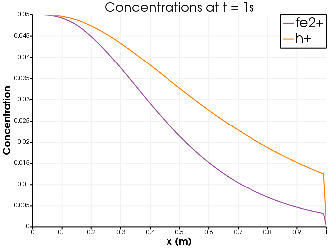
Figure 1: Two of the primary species concentrations at the end of the simulation.
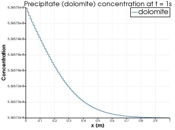
Figure 2: The precipitated dolomite concentration at the end of the simulation.
(modules/porous_flow/examples/tutorial/13.i)
# Example of reactive transport model with dissolution of dolomite
#
# The equilibrium system has 5 primary species (Variables) and
# 5 secondary species (PorousFlowMassFractionAqueousEquilibrium).
# Some of the equilibrium constants have been chosen rather arbitrarily.
#
# Equilibrium reactions
# H+ + HCO3- = CO2(aq)
# -H+ + HCO3- = CO32-
# HCO3- + Ca2+ = CaHCO3+
# HCO3- + Mg2+ = MgHCO3+
# HCO3- + Fe2+ = FeHCO3+
#
# The kinetic reaction that dissolves dolomite involves all 5 primary species.
#
# -2H+ + 2HCO3- + Ca2+ + 0.8Mg2+ + 0.2Fe2+ = CaMg0.8Fe0.2(CO3)2
#
# The initial concentration of precipitated dolomite is high, so it starts
# to dissolve immediately, increasing the concentrations of the primary species.
#
# Only single-phase, fully saturated physics is used.
# The pressure gradient is fixed, so that the Darcy velocity is 0.1m/s.
#
# Primary species are injected from the left side, and they flow to the right.
# Less dolomite dissolution therefore occurs on the left side (where
# the primary species have higher concentration).
#
# This test is more fully documented in tutorial_13
[Mesh]
type = GeneratedMesh
dim = 1
nx = 100
xmax = 1
[]
[Variables]
[h+]
[]
[hco3-]
[]
[ca2+]
[]
[mg2+]
[]
[fe2+]
[]
[]
[AuxVariables]
[eqm_k0]
initial_condition = 2.19E6
[]
[eqm_k1]
initial_condition = 4.73E-11
[]
[eqm_k2]
initial_condition = 0.222
[]
[eqm_k3]
initial_condition = 1E-2
[]
[eqm_k4]
initial_condition = 1E-3
[]
[kinetic_k]
initial_condition = 326.2
[]
[pressure]
[]
[dolomite]
family = MONOMIAL
order = CONSTANT
[]
[dolomite_initial]
initial_condition = 1E-7
[]
[]
[AuxKernels]
[dolomite]
type = PorousFlowPropertyAux
property = mineral_concentration
mineral_species = 0
variable = dolomite
[]
[]
[GlobalParams]
PorousFlowDictator = dictator
gravity = '0 0 0'
[]
[ICs]
[pressure_ic]
type = FunctionIC
variable = pressure
function = '(1 - x) * 1E6'
[]
[h+_ic]
type = BoundingBoxIC
variable = h+
x1 = 0.0
y1 = 0.0
x2 = 1.0e-10
y2 = 0.25
inside = 5.0e-2
outside = 1.0e-6
[]
[hco3_ic]
type = BoundingBoxIC
variable = hco3-
x1 = 0.0
y1 = 0.0
x2 = 1.0e-10
y2 = 0.25
inside = 5.0e-2
outside = 1.0e-6
[]
[ca2_ic]
type = BoundingBoxIC
variable = ca2+
x1 = 0.0
y1 = 0.0
x2 = 1.0e-10
y2 = 0.25
inside = 5.0e-2
outside = 1.0e-6
[]
[mg2_ic]
type = BoundingBoxIC
variable = mg2+
x1 = 0.0
y1 = 0.0
x2 = 1.0e-10
y2 = 0.25
inside = 5.0e-2
outside = 1.0e-6
[]
[fe2_ic]
type = BoundingBoxIC
variable = fe2+
x1 = 0.0
y1 = 0.0
x2 = 1.0e-10
y2 = 0.25
inside = 5.0e-2
outside = 1.0e-6
[]
[]
[Kernels]
[h+_ie]
type = PorousFlowMassTimeDerivative
fluid_component = 0
variable = h+
[]
[h+_conv]
type = PorousFlowAdvectiveFlux
fluid_component = 0
variable = h+
[]
[predis_h+]
type = PorousFlowPreDis
variable = h+
mineral_density = 2875.0
stoichiometry = -2
[]
[hco3-_ie]
type = PorousFlowMassTimeDerivative
fluid_component = 1
variable = hco3-
[]
[hco3-_conv]
type = PorousFlowAdvectiveFlux
fluid_component = 1
variable = hco3-
[]
[predis_hco3-]
type = PorousFlowPreDis
variable = hco3-
mineral_density = 2875.0
stoichiometry = 2
[]
[ca2+_ie]
type = PorousFlowMassTimeDerivative
fluid_component = 2
variable = ca2+
[]
[ca2+_conv]
type = PorousFlowAdvectiveFlux
fluid_component = 2
variable = ca2+
[]
[predis_ca2+]
type = PorousFlowPreDis
variable = ca2+
mineral_density = 2875.0
stoichiometry = 1
[]
[mg2+_ie]
type = PorousFlowMassTimeDerivative
fluid_component = 3
variable = mg2+
[]
[mg2+_conv]
type = PorousFlowAdvectiveFlux
fluid_component = 3
variable = mg2+
[]
[predis_mg2+]
type = PorousFlowPreDis
variable = mg2+
mineral_density = 2875.0
stoichiometry = 0.8
[]
[fe2+_ie]
type = PorousFlowMassTimeDerivative
fluid_component = 4
variable = fe2+
[]
[fe2+_conv]
type = PorousFlowAdvectiveFlux
fluid_component = 4
variable = fe2+
[]
[predis_fe2+]
type = PorousFlowPreDis
variable = fe2+
mineral_density = 2875.0
stoichiometry = 0.2
[]
[]
[UserObjects]
[dictator]
type = PorousFlowDictator
porous_flow_vars = 'h+ hco3- ca2+ mg2+ fe2+'
number_fluid_phases = 1
number_fluid_components = 6
number_aqueous_equilibrium = 5
number_aqueous_kinetic = 1
[]
[]
[FluidProperties]
[simple_fluid]
type = SimpleFluidProperties
viscosity = 1E-3
[]
[]
[BCs]
[hco3-_left]
type = DirichletBC
variable = hco3-
boundary = left
value = 5E-2
[]
[h+_left]
type = DirichletBC
variable = h+
boundary = left
value = 5E-2
[]
[ca2+_left]
type = DirichletBC
variable = ca2+
boundary = left
value = 5E-2
[]
[mg2+_left]
type = DirichletBC
variable = mg2+
boundary = left
value = 5E-2
[]
[fe2+_left]
type = DirichletBC
variable = fe2+
boundary = left
value = 5E-2
[]
[hco3-_right]
type = DirichletBC
variable = hco3-
boundary = right
value = 1E-6
[]
  [h+_right]
    type = DirichletBC
    variable = h+
    boundary = right
    value = 1e-6
  []
[ca2+_right]
type = DirichletBC
variable = ca2+
boundary = right
value = 1E-6
[]
[mg2+_right]
type = DirichletBC
variable = mg2+
boundary = right
value = 1E-6
[]
[fe2+_right]
type = DirichletBC
variable = fe2+
boundary = right
value = 1E-6
[]
[]
[Materials]
[temperature]
type = PorousFlowTemperature
temperature = 298.15
[]
[ppss]
type = PorousFlow1PhaseFullySaturated
porepressure = pressure
[]
[equilibrium_massfrac]
type = PorousFlowMassFractionAqueousEquilibriumChemistry
mass_fraction_vars = 'h+ hco3- ca2+ mg2+ fe2+'
num_reactions = 5
equilibrium_constants = 'eqm_k0 eqm_k1 eqm_k2 eqm_k3 eqm_k4'
primary_activity_coefficients = '1 1 1 1 1'
secondary_activity_coefficients = '1 1 1 1 1'
reactions = '1 1 0 0 0
-1 1 0 0 0
0 1 1 0 0
0 1 0 1 0
0 1 0 0 1'
[]
[kinetic]
type = PorousFlowAqueousPreDisChemistry
primary_concentrations = 'h+ hco3- ca2+ mg2+ fe2+'
num_reactions = 1
equilibrium_constants = kinetic_k
primary_activity_coefficients = '1 1 1 1 1'
reactions = '-2 2 1 0.8 0.2'
specific_reactive_surface_area = '1.2E-8'
kinetic_rate_constant = '3E-4'
activation_energy = '1.5e4'
molar_volume = 64365.0
gas_constant = 8.314
reference_temperature = 298.15
[]
  [dolomite_conc]
    type = PorousFlowAqueousPreDisMineral
    initial_concentrations = dolomite_initial
  []
[simple_fluid]
type = PorousFlowSingleComponentFluid
fp = simple_fluid
phase = 0
[]
[porosity]
type = PorousFlowPorosityConst
porosity = 0.2
[]
[permeability]
type = PorousFlowPermeabilityConst
permeability = '1E-10 0 0 0 1E-10 0 0 0 1E-10'
[]
[relp]
type = PorousFlowRelativePermeabilityConst
phase = 0
[]
[]
[Executioner]
type = Transient
solve_type = Newton
end_time = 1
[TimeStepper]
type = IterationAdaptiveDT
dt = 0.1
[]
[]
[Preconditioning]
active = basic
[basic]
type = SMP
full = true
petsc_options = '-ksp_diagonal_scale -ksp_diagonal_scale_fix'
petsc_options_iname = '-pc_type -sub_pc_type -sub_pc_factor_shift_type -pc_asm_overlap'
petsc_options_value = ' asm lu NONZERO 2'
[]
[preferred_but_might_not_be_installed]
type = SMP
full = true
petsc_options_iname = '-pc_type -pc_factor_mat_solver_package'
petsc_options_value = ' lu mumps'
[]
[]
[Outputs]
print_linear_residuals = false
perf_graph = true
exodus = true
[]
(modules/porous_flow/examples/tutorial/13.i)
# Example of reactive transport model with dissolution of dolomite
#
# The equilibrium system has 5 primary species (Variables) and
# 5 secondary species (PorousFlowMassFractionAqueousEquilibrium).
# Some of the equilibrium constants have been chosen rather arbitrarily.
#
# Equilibrium reactions
# H+ + HCO3- = CO2(aq)
# -H+ + HCO3- = CO32-
# HCO3- + Ca2+ = CaHCO3+
# HCO3- + Mg2+ = MgHCO3+
# HCO3- + Fe2+ = FeHCO3+
#
# The kinetic reaction that dissolves dolomite involves all 5 primary species.
#
# -2H+ + 2HCO3- + Ca2+ + 0.8Mg2+ + 0.2Fe2+ = CaMg0.8Fe0.2(CO3)2
#
# The initial concentration of precipitated dolomite is high, so it starts
# to dissolve immediately, increasing the concentrations of the primary species.
#
# Only single-phase, fully saturated physics is used.
# The pressure gradient is fixed, so that the Darcy velocity is 0.1m/s.
#
# Primary species are injected from the left side, and they flow to the right.
# Less dolomite dissolution therefore occurs on the left side (where
# the primary species have higher concentration).
#
# This test is more fully documented in tutorial_13
[Mesh]
type = GeneratedMesh
dim = 1
nx = 100
xmax = 1
[]
[Variables]
[h+]
[]
[hco3-]
[]
[ca2+]
[]
[mg2+]
[]
[fe2+]
[]
[]
[AuxVariables]
[eqm_k0]
initial_condition = 2.19E6
[]
[eqm_k1]
initial_condition = 4.73E-11
[]
[eqm_k2]
initial_condition = 0.222
[]
[eqm_k3]
initial_condition = 1E-2
[]
[eqm_k4]
initial_condition = 1E-3
[]
[kinetic_k]
initial_condition = 326.2
[]
[pressure]
[]
[dolomite]
family = MONOMIAL
order = CONSTANT
[]
[dolomite_initial]
initial_condition = 1E-7
[]
[]
[AuxKernels]
[dolomite]
type = PorousFlowPropertyAux
property = mineral_concentration
mineral_species = 0
variable = dolomite
[]
[]
[GlobalParams]
PorousFlowDictator = dictator
gravity = '0 0 0'
[]
[ICs]
  [pressure_ic]
    type = FunctionIC
    variable = pressure
    function = '(1 - x) * 1E6'
  []
[h+_ic]
type = BoundingBoxIC
variable = h+
x1 = 0.0
y1 = 0.0
x2 = 1.0e-10
y2 = 0.25
inside = 5.0e-2
outside = 1.0e-6
[]
[hco3_ic]
type = BoundingBoxIC
variable = hco3-
x1 = 0.0
y1 = 0.0
x2 = 1.0e-10
y2 = 0.25
inside = 5.0e-2
outside = 1.0e-6
[]
[ca2_ic]
type = BoundingBoxIC
variable = ca2+
x1 = 0.0
y1 = 0.0
x2 = 1.0e-10
y2 = 0.25
inside = 5.0e-2
outside = 1.0e-6
[]
[mg2_ic]
type = BoundingBoxIC
variable = mg2+
x1 = 0.0
y1 = 0.0
x2 = 1.0e-10
y2 = 0.25
inside = 5.0e-2
outside = 1.0e-6
[]
[fe2_ic]
type = BoundingBoxIC
variable = fe2+
x1 = 0.0
y1 = 0.0
x2 = 1.0e-10
y2 = 0.25
inside = 5.0e-2
outside = 1.0e-6
[]
[]
[Kernels]
[h+_ie]
type = PorousFlowMassTimeDerivative
fluid_component = 0
variable = h+
[]
[h+_conv]
type = PorousFlowAdvectiveFlux
fluid_component = 0
variable = h+
[]
[predis_h+]
type = PorousFlowPreDis
variable = h+
mineral_density = 2875.0
stoichiometry = -2
[]
[hco3-_ie]
type = PorousFlowMassTimeDerivative
fluid_component = 1
variable = hco3-
[]
[hco3-_conv]
type = PorousFlowAdvectiveFlux
fluid_component = 1
variable = hco3-
[]
[predis_hco3-]
type = PorousFlowPreDis
variable = hco3-
mineral_density = 2875.0
stoichiometry = 2
[]
[ca2+_ie]
type = PorousFlowMassTimeDerivative
fluid_component = 2
variable = ca2+
[]
[ca2+_conv]
type = PorousFlowAdvectiveFlux
fluid_component = 2
variable = ca2+
[]
[predis_ca2+]
type = PorousFlowPreDis
variable = ca2+
mineral_density = 2875.0
stoichiometry = 1
[]
[mg2+_ie]
type = PorousFlowMassTimeDerivative
fluid_component = 3
variable = mg2+
[]
[mg2+_conv]
type = PorousFlowAdvectiveFlux
fluid_component = 3
variable = mg2+
[]
[predis_mg2+]
type = PorousFlowPreDis
variable = mg2+
mineral_density = 2875.0
stoichiometry = 0.8
[]
[fe2+_ie]
type = PorousFlowMassTimeDerivative
fluid_component = 4
variable = fe2+
[]
[fe2+_conv]
type = PorousFlowAdvectiveFlux
fluid_component = 4
variable = fe2+
[]
[predis_fe2+]
type = PorousFlowPreDis
variable = fe2+
mineral_density = 2875.0
stoichiometry = 0.2
[]
[]
[UserObjects]
[dictator]
type = PorousFlowDictator
porous_flow_vars = 'h+ hco3- ca2+ mg2+ fe2+'
number_fluid_phases = 1
number_fluid_components = 6
number_aqueous_equilibrium = 5
number_aqueous_kinetic = 1
[]
[]
[FluidProperties]
[simple_fluid]
type = SimpleFluidProperties
viscosity = 1E-3
[]
[]
[BCs]
[hco3-_left]
type = DirichletBC
variable = hco3-
boundary = left
value = 5E-2
[]
[h+_left]
type = DirichletBC
variable = h+
boundary = left
value = 5E-2
[]
[ca2+_left]
type = DirichletBC
variable = ca2+
boundary = left
value = 5E-2
[]
[mg2+_left]
type = DirichletBC
variable = mg2+
boundary = left
value = 5E-2
[]
[fe2+_left]
type = DirichletBC
variable = fe2+
boundary = left
value = 5E-2
[]
[hco3-_right]
type = DirichletBC
variable = hco3-
boundary = right
value = 1E-6
[]
[h+_right]
type = DirichletBC
variable = h+
boundary = right
value = 1e-6
[]
[ca2+_right]
type = DirichletBC
variable = ca2+
boundary = right
value = 1E-6
[]
[mg2+_right]
type = DirichletBC
variable = mg2+
boundary = right
value = 1E-6
[]
[fe2+_right]
type = DirichletBC
variable = fe2+
boundary = right
value = 1E-6
[]
[]
[Materials]
[temperature]
type = PorousFlowTemperature
temperature = 298.15
[]
[ppss]
type = PorousFlow1PhaseFullySaturated
porepressure = pressure
[]
[equilibrium_massfrac]
type = PorousFlowMassFractionAqueousEquilibriumChemistry
mass_fraction_vars = 'h+ hco3- ca2+ mg2+ fe2+'
num_reactions = 5
equilibrium_constants = 'eqm_k0 eqm_k1 eqm_k2 eqm_k3 eqm_k4'
primary_activity_coefficients = '1 1 1 1 1'
secondary_activity_coefficients = '1 1 1 1 1'
reactions = '1 1 0 0 0
-1 1 0 0 0
0 1 1 0 0
0 1 0 1 0
0 1 0 0 1'
[]
[kinetic]
type = PorousFlowAqueousPreDisChemistry
primary_concentrations = 'h+ hco3- ca2+ mg2+ fe2+'
num_reactions = 1
equilibrium_constants = kinetic_k
primary_activity_coefficients = '1 1 1 1 1'
reactions = '-2 2 1 0.8 0.2'
specific_reactive_surface_area = '1.2E-8'
kinetic_rate_constant = '3E-4'
activation_energy = '1.5e4'
molar_volume = 64365.0
gas_constant = 8.314
reference_temperature = 298.15
[]
[dolomite_conc]
type = PorousFlowAqueousPreDisMineral
initial_concentrations = dolomite_initial
[]
[simple_fluid]
type = PorousFlowSingleComponentFluid
fp = simple_fluid
phase = 0
[]
[porosity]
type = PorousFlowPorosityConst
porosity = 0.2
[]
[permeability]
type = PorousFlowPermeabilityConst
permeability = '1E-10 0 0 0 1E-10 0 0 0 1E-10'
[]
[relp]
type = PorousFlowRelativePermeabilityConst
phase = 0
[]
[]
[Executioner]
type = Transient
solve_type = Newton
end_time = 1
[TimeStepper]
type = IterationAdaptiveDT
dt = 0.1
[]
[]
[Preconditioning]
active = basic
[basic]
type = SMP
full = true
petsc_options = '-ksp_diagonal_scale -ksp_diagonal_scale_fix'
petsc_options_iname = '-pc_type -sub_pc_type -sub_pc_factor_shift_type -pc_asm_overlap'
petsc_options_value = ' asm lu NONZERO 2'
[]
[preferred_but_might_not_be_installed]
type = SMP
full = true
petsc_options_iname = '-pc_type -pc_factor_mat_solver_package'
petsc_options_value = ' lu mumps'
[]
[]
[Outputs]
print_linear_residuals = false
perf_graph = true
exodus = true
[]
(modules/porous_flow/examples/tutorial/13.i)
# Example of reactive transport model with dissolution of dolomite
#
# The equilibrium system has 5 primary species (Variables) and
# 5 secondary species (PorousFlowMassFractionAqueousEquilibrium).
# Some of the equilibrium constants have been chosen rather arbitrarily.
#
# Equilibrium reactions
# H+  + HCO3-                      = CO2(aq)
# -H+ + HCO3-                      = CO32-
#       HCO3- + Ca2+               = CaHCO3+
#       HCO3-        + Mg2+        = MgHCO3+
#       HCO3-               + Fe2+ = FeHCO3+
#
# The kinetic reaction that dissolves dolomite involves all 5 primary species.
#
# -2H+ + 2HCO3- + Ca2+ + 0.8Mg2+ + 0.2Fe2+ = CaMg0.8Fe0.2(CO3)2
#
# The initial concentration of precipitated dolomite is high, so it starts
# to dissolve immediately, increasing the concentrations of the primary species.
#
# Only single-phase, fully saturated physics is used.
# The pressure gradient is fixed, so that the Darcy velocity is 0.1m/s.
#
# Primary species are injected from the left side, and they flow to the right.
# Less dolomite dissolution therefore occurs on the left side (where
# the primary species have higher concentration).
#
# This test is more fully documented in tutorial_13
[Mesh]
  type = GeneratedMesh
  dim = 1
  nx = 100
  xmax = 1
[]

[Variables]
  [h+]
  []
  [hco3-]
  []
  [ca2+]
  []
  [mg2+]
  []
  [fe2+]
  []
[]

[AuxVariables]
  [eqm_k0]
    initial_condition = 2.19E6
  []
  [eqm_k1]
    initial_condition = 4.73E-11
  []
  [eqm_k2]
    initial_condition = 0.222
  []
  [eqm_k3]
    initial_condition = 1E-2
  []
  [eqm_k4]
    initial_condition = 1E-3
  []
  [kinetic_k]
    initial_condition = 326.2
  []
  [pressure]
  []
  [dolomite]
    family = MONOMIAL
    order = CONSTANT
  []
  [dolomite_initial]
    initial_condition = 1E-7
  []
[]

[AuxKernels]
  [dolomite]
    type = PorousFlowPropertyAux
    property = mineral_concentration
    mineral_species = 0
    variable = dolomite
  []
[]

[GlobalParams]
  PorousFlowDictator = dictator
  gravity = '0 0 0'
[]

[ICs]
  [pressure_ic]
    type = FunctionIC
    variable = pressure
    function = '(1 - x) * 1E6'
  []
  [h+_ic]
    type = BoundingBoxIC
    variable = h+
    x1 = 0.0
    y1 = 0.0
    x2 = 1.0e-10
    y2 = 0.25
    inside = 5.0e-2
    outside = 1.0e-6
  []
  [hco3_ic]
    type = BoundingBoxIC
    variable = hco3-
    x1 = 0.0
    y1 = 0.0
    x2 = 1.0e-10
    y2 = 0.25
    inside = 5.0e-2
    outside = 1.0e-6
  []
  [ca2_ic]
    type = BoundingBoxIC
    variable = ca2+
    x1 = 0.0
    y1 = 0.0
    x2 = 1.0e-10
    y2 = 0.25
    inside = 5.0e-2
    outside = 1.0e-6
  []
  [mg2_ic]
    type = BoundingBoxIC
    variable = mg2+
    x1 = 0.0
    y1 = 0.0
    x2 = 1.0e-10
    y2 = 0.25
    inside = 5.0e-2
    outside = 1.0e-6
  []
  [fe2_ic]
    type = BoundingBoxIC
    variable = fe2+
    x1 = 0.0
    y1 = 0.0
    x2 = 1.0e-10
    y2 = 0.25
    inside = 5.0e-2
    outside = 1.0e-6
  []
[]

[Kernels]
  [h+_ie]
    type = PorousFlowMassTimeDerivative
    fluid_component = 0
    variable = h+
  []
  [h+_conv]
    type = PorousFlowAdvectiveFlux
    fluid_component = 0
    variable = h+
  []
  [predis_h+]
    type = PorousFlowPreDis
    variable = h+
    mineral_density = 2875.0
    stoichiometry = -2
  []
  [hco3-_ie]
    type = PorousFlowMassTimeDerivative
    fluid_component = 1
    variable = hco3-
  []
  [hco3-_conv]
    type = PorousFlowAdvectiveFlux
    fluid_component = 1
    variable = hco3-
  []
  [predis_hco3-]
    type = PorousFlowPreDis
    variable = hco3-
    mineral_density = 2875.0
    stoichiometry = 2
  []
  [ca2+_ie]
    type = PorousFlowMassTimeDerivative
    fluid_component = 2
    variable = ca2+
  []
  [ca2+_conv]
    type = PorousFlowAdvectiveFlux
    fluid_component = 2
    variable = ca2+
  []
  [predis_ca2+]
    type = PorousFlowPreDis
    variable = ca2+
    mineral_density = 2875.0
    stoichiometry = 1
  []
  [mg2+_ie]
    type = PorousFlowMassTimeDerivative
    fluid_component = 3
    variable = mg2+
  []
  [mg2+_conv]
    type = PorousFlowAdvectiveFlux
    fluid_component = 3
    variable = mg2+
  []
  [predis_mg2+]
    type = PorousFlowPreDis
    variable = mg2+
    mineral_density = 2875.0
    stoichiometry = 0.8
  []
  [fe2+_ie]
    type = PorousFlowMassTimeDerivative
    fluid_component = 4
    variable = fe2+
  []
  [fe2+_conv]
    type = PorousFlowAdvectiveFlux
    fluid_component = 4
    variable = fe2+
  []
  [predis_fe2+]
    type = PorousFlowPreDis
    variable = fe2+
    mineral_density = 2875.0
    stoichiometry = 0.2
  []
[]

[UserObjects]
  [dictator]
    type = PorousFlowDictator
    porous_flow_vars = 'h+ hco3- ca2+ mg2+ fe2+'
    number_fluid_phases = 1
    number_fluid_components = 6
    number_aqueous_equilibrium = 5
    number_aqueous_kinetic = 1
  []
[]

[FluidProperties]
  [simple_fluid]
    type = SimpleFluidProperties
    viscosity = 1E-3
  []
[]

[BCs]
  [hco3-_left]
    type = DirichletBC
    variable = hco3-
    boundary = left
    value = 5E-2
  []
  [h+_left]
    type = DirichletBC
    variable = h+
    boundary = left
    value = 5E-2
  []
  [ca2+_left]
    type = DirichletBC
    variable = ca2+
    boundary = left
    value = 5E-2
  []
  [mg2+_left]
    type = DirichletBC
    variable = mg2+
    boundary = left
    value = 5E-2
  []
  [fe2+_left]
    type = DirichletBC
    variable = fe2+
    boundary = left
    value = 5E-2
  []
  [hco3-_right]
    type = DirichletBC
    variable = hco3-
    boundary = right
    value = 1E-6
  []
  [h+_right]
    type = DirichletBC
    variable = h+
    boundary = right
    value = 1e-6
  []
  [ca2+_right]
    type = DirichletBC
    variable = ca2+
    boundary = right
    value = 1E-6
  []
  [mg2+_right]
    type = DirichletBC
    variable = mg2+
    boundary = right
    value = 1E-6
  []
  [fe2+_right]
    type = DirichletBC
    variable = fe2+
    boundary = right
    value = 1E-6
  []
[]

[Materials]
  [temperature]
    type = PorousFlowTemperature
    temperature = 298.15
  []
  [ppss]
    type = PorousFlow1PhaseFullySaturated
    porepressure = pressure
  []
  [equilibrium_massfrac]
    type = PorousFlowMassFractionAqueousEquilibriumChemistry
    mass_fraction_vars = 'h+ hco3- ca2+ mg2+ fe2+'
    num_reactions = 5
    equilibrium_constants = 'eqm_k0 eqm_k1 eqm_k2 eqm_k3 eqm_k4'
    primary_activity_coefficients = '1 1 1 1 1'
    secondary_activity_coefficients = '1 1 1 1 1'
    reactions = '1 1 0 0 0
                -1 1 0 0 0
                 0 1 1 0 0
                 0 1 0 1 0
                 0 1 0 0 1'
  []
  [kinetic]
    type = PorousFlowAqueousPreDisChemistry
    primary_concentrations = 'h+ hco3- ca2+ mg2+ fe2+'
    num_reactions = 1
    equilibrium_constants = kinetic_k
    primary_activity_coefficients = '1 1 1 1 1'
    reactions = '-2 2 1 0.8 0.2'
    specific_reactive_surface_area = '1.2E-8'
    kinetic_rate_constant = '3E-4'
    activation_energy = '1.5e4'
    molar_volume = 64365.0
    gas_constant = 8.314
    reference_temperature = 298.15
  []
  [dolomite_conc]
    type = PorousFlowAqueousPreDisMineral
    initial_concentrations = dolomite_initial
  []
  [simple_fluid]
    type = PorousFlowSingleComponentFluid
    fp = simple_fluid
    phase = 0
  []
  [porosity]
    type = PorousFlowPorosityConst
    porosity = 0.2
  []
  [permeability]
    type = PorousFlowPermeabilityConst
    permeability = '1E-10 0 0 0 1E-10 0 0 0 1E-10'
  []
  [relp]
    type = PorousFlowRelativePermeabilityConst
    phase = 0
  []
[]

[Executioner]
  type = Transient
  solve_type = Newton
  end_time = 1
  [TimeStepper]
    type = IterationAdaptiveDT
    dt = 0.1
  []
[]

[Preconditioning]
  active = basic
  [basic]
    type = SMP
    full = true
    petsc_options = '-ksp_diagonal_scale -ksp_diagonal_scale_fix'
    petsc_options_iname = '-pc_type -sub_pc_type -sub_pc_factor_shift_type -pc_asm_overlap'
    petsc_options_value = ' asm      lu           NONZERO                   2'
  []
  [preferred_but_might_not_be_installed]
    type = SMP
    full = true
    petsc_options_iname = '-pc_type -pc_factor_mat_solver_package'
    petsc_options_value = ' lu       mumps'
  []
[]

[Outputs]
  print_linear_residuals = false
  perf_graph = true
  exodus = true
[]