Porous Flow Tutorial Page 03. Adding heat advection and conduction

This Page adds heat conduction and advection with the fluid. The differential equation governing the temperature evolution is (1)

This equation is nonlinear since there are products of and , as well as the nonlinear function . Most of the nomenclature was used in Page 01, and the additional symbols introduced are:

• is time (units s)

• is the density of the rock grains (units kg.m)

• is the specific heat capacity of the rock grains (units J.kg.K)

• is the temperature (units K)

• is the specific heat capacity of the fluid (units J.kg.K)

• is the thermal conductivity of the rock-fluid system (units J.s.m.K). It is a tensor.

Before attempting to write an input file, a rough estimate of the expected nonlinear residuals must be performed, as discussed in convergence criteria. The residual for the Eq. (1) is approximately

where the parameters , , , , and , have been used in the final expression. In Page 02 the choice Pa.m was made. Choosing K.m yields

Note that this is significantly greater than the for the fluid equation. In the main, MOOSE can handle these types of discrepancies, but it is good practise to scale the variables so that their residuals are of similar magnitude. Therefore, a scaling factor of is applied to the temperature variable.

To model this thermo-hydro system, the PorousFlowBasicTHM action needs to be enhanced to read:

[Variables<<<{"href": "../../syntax/Variables/index.html"}>>>]
  [porepressure]
  []
  [temperature]
    initial_condition<<<{"description": "Specifies a constant initial condition for this variable"}>>> = 293
    scaling<<<{"description": "Specifies a scaling factor to apply to this variable"}>>> = 1E-8
  []
[]

[PorousFlowBasicTHM<<<{"href": "../../syntax/PorousFlowBasicTHM/index.html"}>>>]
  porepressure<<<{"description": "The name of the porepressure variable"}>>> = porepressure
  temperature<<<{"description": "For isothermal simulations, this is the temperature at which fluid properties (and stress-free strains) are evaluated at.  Otherwise, this is the name of the temperature variable.  Units = Kelvin"}>>> = temperature
  coupling_type<<<{"description": "The type of simulation.  For simulations involving Mechanical deformations, you will need to supply the correct Biot coefficient.  For simulations involving Thermal flows, you will need an associated ConstantThermalExpansionCoefficient Material"}>>> = ThermoHydro
  gravity<<<{"description": "Gravitational acceleration vector downwards (m/s^2)"}>>> = '0 0 0'
  fp<<<{"description": "The name of the user object for fluid properties. Only needed if fluid_properties_type = PorousFlowSingleComponentFluid"}>>> = the_simple_fluid
[]

and some extra properties need to be added to the SimpleFluidProperties:

[FluidProperties<<<{"href": "../../syntax/FluidProperties/index.html"}>>>]
  [the_simple_fluid]
    type = SimpleFluidProperties<<<{"description": "Fluid properties for a simple fluid with a constant bulk density", "href": "../../source/fluidproperties/SimpleFluidProperties.html"}>>>
    bulk_modulus<<<{"description": "Constant bulk modulus (Pa)"}>>> = 2E9
    viscosity<<<{"description": "Constant dynamic viscosity (Pa.s)"}>>> = 1.0E-3
    density0<<<{"description": "Density at zero pressure and zero temperature"}>>> = 1000.0
    thermal_expansion<<<{"description": "Constant coefficient of thermal expansion (1/K)"}>>> = 0.0002
    cp<<<{"description": "Constant specific heat capacity at constant pressure (J/kg/K)"}>>> = 4194
    cv<<<{"description": "Constant specific heat capacity at constant volume (J/kg/K)"}>>> = 4186
    porepressure_coefficient<<<{"description": "The enthalpy is internal_energy + P / density * porepressure_coefficient.  Physically this should be 1.0, but analytic solutions are simplified when it is zero"}>>> = 0
  []
[]

The boundary conditions used are the same as in Page 01 in addition to specifying a constant injection temperature of 313K:

[BCs<<<{"href": "../../syntax/BCs/index.html"}>>>]
  [constant_injection_porepressure]
    type = DirichletBC<<<{"description": "Imposes the essential boundary condition $u=g$, where $g$ is a constant, controllable value.", "href": "../../source/bcs/DirichletBC.html"}>>>
    variable<<<{"description": "The name of the variable that this residual object operates on"}>>> = porepressure
    value<<<{"description": "Value of the BC"}>>> = 1E6
    boundary<<<{"description": "The list of boundary IDs from the mesh where this object applies"}>>> = injection_area
  []
  [constant_injection_temperature]
    type = DirichletBC<<<{"description": "Imposes the essential boundary condition $u=g$, where $g$ is a constant, controllable value.", "href": "../../source/bcs/DirichletBC.html"}>>>
    variable<<<{"description": "The name of the variable that this residual object operates on"}>>> = temperature
    value<<<{"description": "Value of the BC"}>>> = 313
    boundary<<<{"description": "The list of boundary IDs from the mesh where this object applies"}>>> = injection_area
  []
[]

Finally, some temperature-related Materials need to be defined

  [thermal_expansion]
    type = PorousFlowConstantThermalExpansionCoefficient
    biot_coefficient = 0.8
    drained_coefficient = 0.003
    fluid_coefficient = 0.0002
  []
  [rock_internal_energy]
    type = PorousFlowMatrixInternalEnergy
    density = 2500.0
    specific_heat_capacity = 1200.0
  []
  [thermal_conductivity]
    type = PorousFlowThermalConductivityIdeal
    dry_thermal_conductivity = '10 0 0  0 10 0  0 0 10'
    block = 'caps aquifer'
  []
[]

An animation of the results is shown in Figure 1. Readers are encouraged pause and explore the effect of changing parameters such as the rock thermal conductivity.

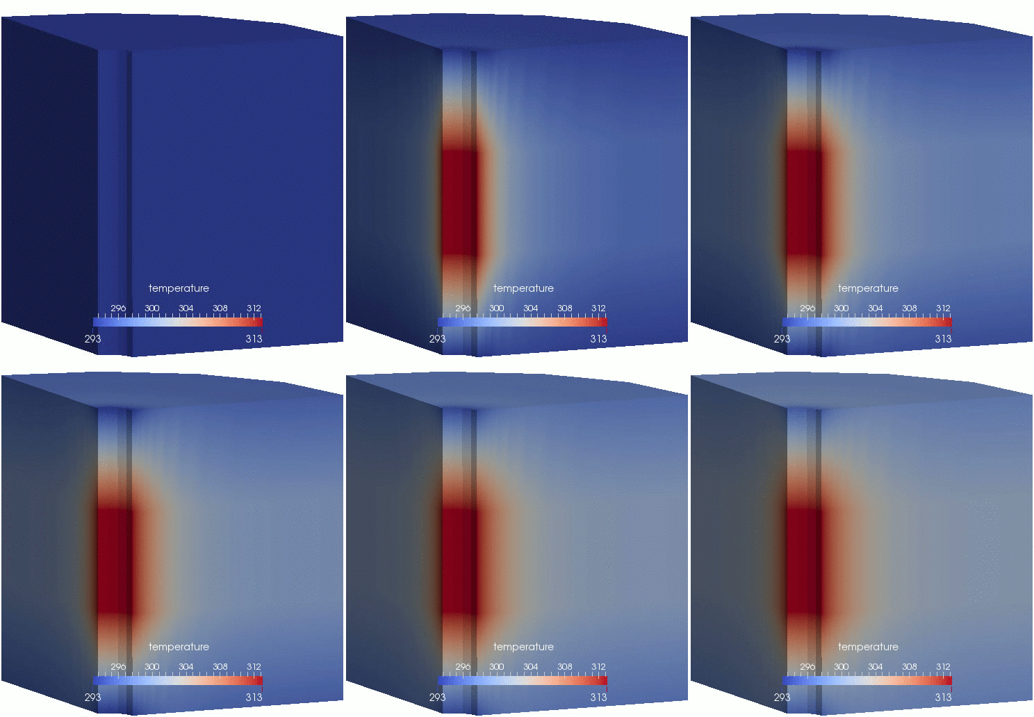
Figure 1: Temperature evolution in the borehole-aquifer-caprock system.

Start | Previous | Next