Rotating Circle

Level Set Equation

Figure 1 show the results of solving the rotating bubble problem with the level set equation alone, which initially behaves in a consistent manner. However, near the end of the simulation node-to-node oscillations appear in the solution, which is evident in the contour lines shown in Figure 1. As expected, these oscillations influence the area of the region encapsulated by the 0.5 level set contour as shown in Figure 4 and discussed in the Area Comparison section.

The complete input file for running this portion of the example is included below and it may be executed as follows.

cd ~/projects/moose/module/level_set/examples/rotating_circle
../../level_set-opt -i rotating_circle.i

[Mesh]
  type = GeneratedMesh
  dim = 2
  xmin = -1
  xmax = 1
  ymin = -1
  ymax = 1
  nx = 32
  ny = 32
  uniform_refine = 2
[]

[AuxVariables]
  [./velocity]
    family = LAGRANGE_VEC
  [../]
[]

[Variables]
  [./phi]
  [../]
[]

[Functions]
  [./phi_exact]
    type = LevelSetOlssonBubble
    epsilon = 0.03
    center = '0 0.5 0'
    radius = 0.15
  [../]
  [./velocity_func]
    type = ParsedVectorFunction
    expression_x = '4*y'
    expression_y = '-4*x'
  [../]
[]

[ICs]
  [./phi_ic]
    type = FunctionIC
    function = phi_exact
    variable = phi
  [../]
  [./vel_ic]
    type = VectorFunctionIC
    variable = velocity
    function = velocity_func
  []
[]

[Kernels]
  [./time]
    type = TimeDerivative
    variable = phi
  [../]

  [./advection]
    type = LevelSetAdvection
    velocity = velocity
    variable = phi
  [../]
[]

[Postprocessors]
  [./area]
    type = LevelSetVolume
    threshold = 0.5
    variable = phi
    location = outside
    execute_on = 'initial timestep_end'
  [../]
  [./cfl]
    type = LevelSetCFLCondition
    velocity = velocity
    execute_on = 'initial' #timestep_end'
  [../]
[]

[Executioner]
  type = Transient
  solve_type = PJFNK
  start_time = 0
  end_time = 1.570796
  scheme = crank-nicolson
  petsc_options_iname = '-pc_type -pc_sub_type'
  petsc_options_value = 'asm      ilu'
  [./TimeStepper]
    type = PostprocessorDT
    postprocessor = cfl
    scale = 0.8
  [../]
[]

[Outputs]
  csv = true
  exodus = true
[]

Level Set Equation with SUPG

Adding SUPG stabilization—set the theory for details—mitigates the oscillations present in the first step, as shown in Figure 2. Adding the SUPG stabilization is trivial simply add the time and advection SUPG kernels to the input file ((modules/level_set/examples/rotating_circle/circle_rotate_supg.i)) shown previously, the kernels block will then appear as:

[Kernels]
  [./time]
    type = TimeDerivative
    variable = phi
  [../]
  [./advection]
    type = LevelSetAdvection
    velocity = velocity
    variable = phi
  [../]
  [./advection_supg]
    type = LevelSetAdvectionSUPG
    velocity = velocity
    variable = phi
  [../]
  [./time_supg]
    type = LevelSetTimeDerivativeSUPG
    velocity = velocity
    variable = phi
  [../]
[]

Adding the stabilization improve the numerical solution but it suffers from a loss of conservation of the phase field variable, as discussed in the Area Comparison section and shown in Figure 4.

Level Set Equation with Reinitialization

Adding reinitialization, in this case the scheme proposed by Olsson et al. (2007), requires the use of the MOOSE MultiApp. The enable reinitialization two input files are required: a parent and sub-application.

The parent input file must add the necessary MultiApps and Transfers blocks. For the problem at hand ((modules/level_set/examples/rotating_circle/circle_rotate_parent.i)) this easily accomplished by adding the following to the input file from the first step (i.e., do not include the SUPG kernels).

[MultiApps]
  [./reinit]
    type = LevelSetReinitializationMultiApp
    input_files = 'circle_rotate_sub.i'
    execute_on = 'timestep_end'
  [../]
[]

[Transfers]
  [./to_sub]
    type = MultiAppCopyTransfer
    source_variable = phi
    variable = phi
    to_multi_app = reinit
    execute_on = 'timestep_end'
  [../]
  [./to_sub_init]
    type = MultiAppCopyTransfer
    source_variable = phi
    variable = phi_0
    to_multi_app = reinit
    execute_on = 'timestep_end'
  [../]
  [./from_sub]
    type = MultiAppCopyTransfer
    source_variable = phi
    variable = phi
    from_multi_app = reinit
    execute_on = 'timestep_end'
  [../]
[]

Next, the sub-application input file must be created, which is shown below. This input file mimics the parent input file closely, with three notable exceptions. First, the Kernels block utilize the time derivative and a new object, LevelSetOlssonReinitialization, that implements the reinitialization scheme of Olsson et al. (2007). Second, the Problem is set to use the LevelSetReinitializationProblem. Finally, the UserObjects block includes a terminator, LevelSetOlssonTerminator, which is responsible for stopping the reinitialization solve when steady-state is achieved according to the criteria defined by Olsson et al. (2007).

[Mesh]
  type = GeneratedMesh
  dim = 2
  xmin = -1
  xmax = 1
  ymin = -1
  ymax = 1
  nx = 32
  ny = 32
  uniform_refine = 2
[]

[Variables]
  [./phi]
  [../]
[]

[AuxVariables]
  [./phi_0]
  [../]
  [./marker]
  [../]
[]

[Kernels]
  [./time]
    type = TimeDerivative
    variable = phi
  [../]
  [./reinit]
    type = LevelSetOlssonReinitialization
    variable = phi
    phi_0 = phi_0
    epsilon = 0.03
  [../]
[]

[Problem]
  type = LevelSetReinitializationProblem
[]

[UserObjects]
  [./arnold]
    type = LevelSetOlssonTerminator
    tol = 1
    min_steps = 3
  [../]
[]

[Executioner]
  type = Transient
  solve_type = NEWTON
  start_time = 0
  num_steps = 100
  nl_abs_tol = 1e-14
  scheme = crank-nicolson
  line_search = none
  petsc_options_iname = '-pc_type -pc_sub_type'
  petsc_options_value = 'asm      ilu'
  dt = 0.003
[]

[Outputs]
[]

Figure 3 shows the results of the bubble problem with reinitialization, the result looks similar to the SUPG result. However, if you consider the area conservation discussed in the Area Comparison section, the reinitialization scheme yields the superior solution for this problem.

Area Comparison

Figure 4 is a plot of the area of the circle during the three simulations. Note that in the unstabilized, un-reinitialized level set equation, both area conservation and stability issues are readily apparent. The instabilities are especially obvious in Figure 4, where the drastic area changes are due to numerical oscillations in the solution field. Adding SUPG stabilization helps ameliorate the stability concern but it suffers from loss of area conservation. The re-initialization scheme is both stable and area-conserving.

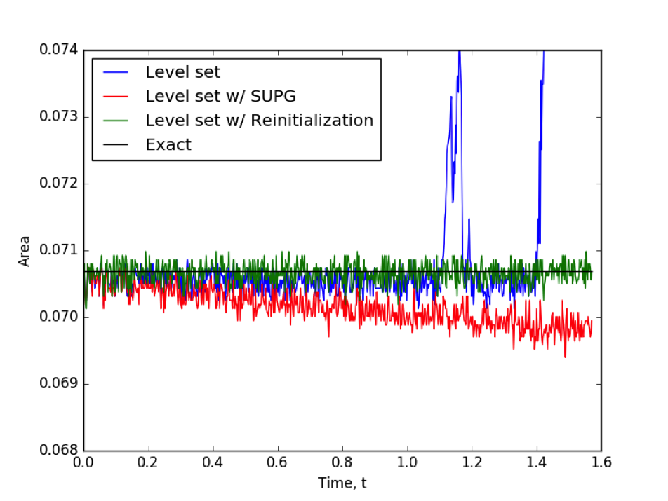
Figure 4: Comparison of area inside the bubble during simulations.

The re-initialization methods performs well, but it is computationally expensive and picking the pseudo timestep size , steady-state criteria , and interface thickness correctly for the re-initialization problem is a non-trivial difficulty. Nevertheless, the level set module provides a valuable starting point and proof-of-concept for other researchers interested in the method, and the existing algorithm can no doubt be tuned to the needs of specific applications in terms of conservation and computational cost requirements.

References

- Elin Olsson, Gunilla Kreiss, and Sara Zahedi.
A conservative level set method for two phase flow ii.
Journal of Computational Physics, 225(1):785–807, 2007.
URL: http://dx.doi.org/10.1016/j.jcp.2006.12.027.[Export]