Example 3a: Nonlinear Site-Response Analysis

This example demonstrates a nonlinear site-response analysis using I-soil. A 20 m soil column is created and meshed to have 20 elements, each measuring 1 m x 1 m x 1 m. Shear wave velocity (and the small-strain shear modulus) is depth dependent and has a value of 100 m/sec at top and 250 m/sec at the bottom. Figure 1 demonstrates the geometry of the problem.

Figure 1: Schematic of the non-uniform shear beam model (reprinted from Baltaji et al. (2017)).

Below is the full input file provided to run this analysis.

[Mesh<<<{"href": "../syntax/Mesh/index.html"}>>>]
  type = GeneratedMesh
  nx = 1
  ny = 1
  nz = 20
  xmin = -0.5
  ymin = -0.5
  zmin = 0.0
  xmax = 0.5
  ymax = 0.5
  zmax = 20.0
  dim = 3
[]

[GlobalParams<<<{"href": "../syntax/GlobalParams/index.html"}>>>]
  displacements = 'disp_x disp_y disp_z'
[]

[Variables<<<{"href": "../syntax/Variables/index.html"}>>>]
  [./disp_x]
  [../]
  [./disp_y]
  [../]
  [./disp_z]
  [../]
[]

[AuxVariables<<<{"href": "../syntax/AuxVariables/index.html"}>>>]
  [./vel_x]
  [../]
  [./accel_x]
  [../]
  [./vel_y]
  [../]
  [./accel_y]
  [../]
  [./vel_z]
  [../]
  [./accel_z]
  [../]
  [./layer_id]
    order<<<{"description": "Specifies the order of the FE shape function to use for this variable (additional orders not listed are allowed)"}>>> = CONSTANT
    family<<<{"description": "Specifies the family of FE shape functions to use for this variable"}>>> = MONOMIAL
  [../]
[]

[Kernels<<<{"href": "../syntax/Kernels/index.html"}>>>]
  [./DynamicTensorMechanics<<<{"href": "../syntax/Kernels/DynamicTensorMechanics/index.html"}>>>]
    displacements<<<{"description": "The nonlinear displacement variables for the problem"}>>> = 'disp_x disp_y disp_z'
    stiffness_damping_coefficient<<<{"description": "Name of material property or a constant real number defining stiffness Rayleigh parameter (zeta)."}>>> = 0.000781
  [../]
  [./inertia_x]
    type = InertialForce<<<{"description": "Calculates the residual for the inertial force ($M \\cdot acceleration$) and the contribution of mass dependent Rayleigh damping and HHT time  integration scheme ($\\eta \\cdot M \\cdot ((1+\\alpha)velq2-\\alpha \\cdot vel-old) $)", "href": "../source/kernels/InertialForce.html"}>>>
    variable<<<{"description": "The name of the variable that this residual object operates on"}>>> = disp_x
    velocity<<<{"description": "velocity variable"}>>> = vel_x
    acceleration<<<{"description": "acceleration variable"}>>> = accel_x
    beta<<<{"description": "beta parameter for Newmark Time integration"}>>> = 0.25
    gamma<<<{"description": "gamma parameter for Newmark Time integration"}>>> = 0.5
    eta<<<{"description": "Name of material property or a constant real number defining the eta parameter for the Rayleigh damping."}>>> = 0.64026
  [../]
  [./inertia_y]
    type = InertialForce<<<{"description": "Calculates the residual for the inertial force ($M \\cdot acceleration$) and the contribution of mass dependent Rayleigh damping and HHT time  integration scheme ($\\eta \\cdot M \\cdot ((1+\\alpha)velq2-\\alpha \\cdot vel-old) $)", "href": "../source/kernels/InertialForce.html"}>>>
    variable<<<{"description": "The name of the variable that this residual object operates on"}>>> = disp_y
    velocity<<<{"description": "velocity variable"}>>> = vel_y
    acceleration<<<{"description": "acceleration variable"}>>> = accel_y
    beta<<<{"description": "beta parameter for Newmark Time integration"}>>> = 0.25
    gamma<<<{"description": "gamma parameter for Newmark Time integration"}>>> = 0.5
    eta<<<{"description": "Name of material property or a constant real number defining the eta parameter for the Rayleigh damping."}>>> = 0.64026
  [../]
  [./inertia_z]
    type = InertialForce<<<{"description": "Calculates the residual for the inertial force ($M \\cdot acceleration$) and the contribution of mass dependent Rayleigh damping and HHT time  integration scheme ($\\eta \\cdot M \\cdot ((1+\\alpha)velq2-\\alpha \\cdot vel-old) $)", "href": "../source/kernels/InertialForce.html"}>>>
    variable<<<{"description": "The name of the variable that this residual object operates on"}>>> = disp_z
    velocity<<<{"description": "velocity variable"}>>> = vel_z
    acceleration<<<{"description": "acceleration variable"}>>> = accel_z
    beta<<<{"description": "beta parameter for Newmark Time integration"}>>> = 0.25
    gamma<<<{"description": "gamma parameter for Newmark Time integration"}>>> = 0.5
    eta<<<{"description": "Name of material property or a constant real number defining the eta parameter for the Rayleigh damping."}>>> = 0.64026
  [../]
  [./gravity]
    type = Gravity<<<{"description": "Apply gravity. Value is in units of acceleration.", "href": "../source/kernels/Gravity.html"}>>>
    variable<<<{"description": "The name of the variable that this residual object operates on"}>>> = disp_z
    value<<<{"description": "Value multiplied against the residual, e.g. gravitational acceleration"}>>> = -9.81
  [../]
[]

[AuxKernels<<<{"href": "../syntax/AuxKernels/index.html"}>>>]
  [./accel_x]
    type = NewmarkAccelAux<<<{"description": "Computes the current acceleration using the Newmark method.", "href": "../source/auxkernels/NewmarkAccelAux.html"}>>>
    variable<<<{"description": "The name of the variable that this object applies to"}>>> = accel_x
    displacement<<<{"description": "displacement variable"}>>> = disp_x
    velocity<<<{"description": "velocity variable"}>>> = vel_x
    beta<<<{"description": "beta parameter for Newmark method"}>>> = 0.25
    execute_on<<<{"description": "The list of flag(s) indicating when this object should be executed. For a description of each flag, see https://mooseframework.inl.gov/source/interfaces/SetupInterface.html."}>>> = timestep_end
  [../]
  [./vel_x]
    type = NewmarkVelAux<<<{"description": "Calculates the current velocity using Newmark method.", "href": "../source/auxkernels/NewmarkVelAux.html"}>>>
    variable<<<{"description": "The name of the variable that this object applies to"}>>> = vel_x
    acceleration<<<{"description": "acceleration variable"}>>> = accel_x
    gamma<<<{"description": "gamma parameter for Newmark method"}>>> = 0.5
    execute_on<<<{"description": "The list of flag(s) indicating when this object should be executed. For a description of each flag, see https://mooseframework.inl.gov/source/interfaces/SetupInterface.html."}>>> = timestep_end
  [../]
  [./accel_y]
    type = NewmarkAccelAux<<<{"description": "Computes the current acceleration using the Newmark method.", "href": "../source/auxkernels/NewmarkAccelAux.html"}>>>
    variable<<<{"description": "The name of the variable that this object applies to"}>>> = accel_y
    displacement<<<{"description": "displacement variable"}>>> = disp_y
    velocity<<<{"description": "velocity variable"}>>> = vel_y
    beta<<<{"description": "beta parameter for Newmark method"}>>> = 0.25
    execute_on<<<{"description": "The list of flag(s) indicating when this object should be executed. For a description of each flag, see https://mooseframework.inl.gov/source/interfaces/SetupInterface.html."}>>> = timestep_end
  [../]
  [./vel_y]
    type = NewmarkVelAux<<<{"description": "Calculates the current velocity using Newmark method.", "href": "../source/auxkernels/NewmarkVelAux.html"}>>>
    variable<<<{"description": "The name of the variable that this object applies to"}>>> = vel_y
    acceleration<<<{"description": "acceleration variable"}>>> = accel_y
    gamma<<<{"description": "gamma parameter for Newmark method"}>>> = 0.5
    execute_on<<<{"description": "The list of flag(s) indicating when this object should be executed. For a description of each flag, see https://mooseframework.inl.gov/source/interfaces/SetupInterface.html."}>>> = timestep_end
  [../]
  [./accel_z]
    type = NewmarkAccelAux<<<{"description": "Computes the current acceleration using the Newmark method.", "href": "../source/auxkernels/NewmarkAccelAux.html"}>>>
    variable<<<{"description": "The name of the variable that this object applies to"}>>> = accel_z
    displacement<<<{"description": "displacement variable"}>>> = disp_z
    velocity<<<{"description": "velocity variable"}>>> = vel_z
    beta<<<{"description": "beta parameter for Newmark method"}>>> = 0.25
    execute_on<<<{"description": "The list of flag(s) indicating when this object should be executed. For a description of each flag, see https://mooseframework.inl.gov/source/interfaces/SetupInterface.html."}>>> = timestep_end
  [../]
  [./vel_z]
    type = NewmarkVelAux<<<{"description": "Calculates the current velocity using Newmark method.", "href": "../source/auxkernels/NewmarkVelAux.html"}>>>
    variable<<<{"description": "The name of the variable that this object applies to"}>>> = vel_z
    acceleration<<<{"description": "acceleration variable"}>>> = accel_z
    gamma<<<{"description": "gamma parameter for Newmark method"}>>> = 0.5
    execute_on<<<{"description": "The list of flag(s) indicating when this object should be executed. For a description of each flag, see https://mooseframework.inl.gov/source/interfaces/SetupInterface.html."}>>> = timestep_end
  [../]
  [./layer_id]
     type = UniformLayerAuxKernel<<<{"description": "Computes an AuxVariable for representing a layered structure in an arbitrary direction.", "href": "../source/auxkernels/UniformLayerAuxKernel.html"}>>>
     variable<<<{"description": "The name of the variable that this object applies to"}>>> = layer_id
     interfaces<<<{"description": "A list of layer interface locations to apply across the domain in the specified direction."}>>> = '1 2 3 4 5 6 7 8 9 10 11 12 13 14 15 16 17 18 19 20.2'
     direction<<<{"description": "The direction to apply layering."}>>> = '0.0 0.0 1.0'
     execute_on<<<{"description": "The list of flag(s) indicating when this object should be executed. For a description of each flag, see https://mooseframework.inl.gov/source/interfaces/SetupInterface.html."}>>> = initial
  [../]
[]

[BCs<<<{"href": "../syntax/BCs/index.html"}>>>]
  [./bottom_z]
    type = DirichletBC<<<{"description": "Imposes the essential boundary condition $u=g$, where $g$ is a constant, controllable value.", "href": "../source/bcs/DirichletBC.html"}>>>
    variable<<<{"description": "The name of the variable that this residual object operates on"}>>> = disp_z
    boundary<<<{"description": "The list of boundary IDs from the mesh where this object applies"}>>> = 'back'
    value<<<{"description": "Value of the BC"}>>> = 0.0
  [../]
  [./bottom_y]
    type = DirichletBC<<<{"description": "Imposes the essential boundary condition $u=g$, where $g$ is a constant, controllable value.", "href": "../source/bcs/DirichletBC.html"}>>>
    variable<<<{"description": "The name of the variable that this residual object operates on"}>>> = disp_y
    boundary<<<{"description": "The list of boundary IDs from the mesh where this object applies"}>>> = 'back'
    value<<<{"description": "Value of the BC"}>>> = 0.0
  [../]
  [./bottom_accel]
    type = PresetAcceleration<<<{"description": "Prescribe acceleration on a given boundary in a given direction", "href": "../source/bcs/PresetAcceleration.html"}>>>
    boundary<<<{"description": "The list of boundary IDs from the mesh where this object applies"}>>> = 'back'
    function<<<{"description": "Function describing the velocity."}>>> = accel_bottom
    variable<<<{"description": "The name of the variable that this residual object operates on"}>>> = 'disp_x'
    beta<<<{"description": "beta parameter for Newmark time integration."}>>> = 0.25
    acceleration<<<{"description": "The acceleration variable."}>>> = 'accel_x'
    velocity<<<{"description": "The velocity variable."}>>> = 'vel_x'
  [../]
  [./Periodic<<<{"href": "../syntax/BCs/Periodic/index.html"}>>>]
    [./y_dir]
      variable<<<{"description": "Variable for the periodic boundary condition"}>>> = 'disp_x disp_y disp_z'
      primary<<<{"description": "Boundary ID associated with the primary boundary."}>>> = 'bottom'
      secondary<<<{"description": "Boundary ID associated with the secondary boundary."}>>> = 'top'
      translation<<<{"description": "Vector that translates coordinates on the primary boundary to coordinates on the secondary boundary."}>>> = '0.0 1.0 0.0'
    [../]
    [./x_dir]
      variable<<<{"description": "Variable for the periodic boundary condition"}>>> = 'disp_x disp_y disp_z'
      primary<<<{"description": "Boundary ID associated with the primary boundary."}>>> = 'left'
      secondary<<<{"description": "Boundary ID associated with the secondary boundary."}>>> = 'right'
      translation<<<{"description": "Vector that translates coordinates on the primary boundary to coordinates on the secondary boundary."}>>> = '1.0 0.0 0.0'
    [../]
  [../]
[]

[Functions<<<{"href": "../syntax/Functions/index.html"}>>>]
  [./accel_bottom]
     type = PiecewiseLinear<<<{"description": "Linearly interpolates between pairs of x-y data", "href": "../source/functions/PiecewiseLinear.html"}>>>
     data_file<<<{"description": "File holding CSV data"}>>> = chichi_bc_mpss_xp20.csv
     format<<<{"description": "Format of csv data file that is in either in columns or rows"}>>> = 'columns'
  [../]
  [./initial_zz]
    type = ParsedFunction<<<{"description": "Function created by parsing a string", "href": "../source/functions/MooseParsedFunction.html"}>>>
    value<<<{"description": "The user defined function."}>>> = '-2000.0 * 9.81 * (20.0 - z)'
  [../]
  [./initial_xx]
    type = ParsedFunction<<<{"description": "Function created by parsing a string", "href": "../source/functions/MooseParsedFunction.html"}>>>
    value<<<{"description": "The user defined function."}>>> = '-2000.0 * 9.81 * (20.0 - z) * 0.3/0.7'
  [../]
[]

[Materials<<<{"href": "../syntax/Materials/index.html"}>>>]
  [./I_Soil<<<{"href": "../syntax/Materials/I_Soil/index.html"}>>>]
    [./soil_all]
       block<<<{"description": "The blocks where this material model is applied."}>>> = 0
       layer_variable<<<{"description": "The auxvariable providing the soil layer identification."}>>> = layer_id
       layer_ids<<<{"description": "Vector of layer ids that map one-to-one to the rest of the soil layer parameters provided as input."}>>> = '0 1 2 3 4 5 6 7 8 9 10 11 12 13 14 15 16 17 18 19'
       initial_soil_stress<<<{"description": "The function values for the initial stress distribution. 9 function names have to be provided corresponding to stress_xx, stress_xy, stress_xz, stress_yx, stress_yy, stress_yz, stress_zx, stress_zy, stress_zz. Each function can be a function of space."}>>> = 'initial_xx 0 0 0 initial_xx 0 0 0 initial_zz'
       poissons_ratio<<<{"description": "Poissons's ratio for the soil layers. The size of the vector should be same as the size of layer_ids."}>>> = '0.3 0.3 0.3 0.3 0.3 0.3 0.3 0.3 0.3 0.3 0.3 0.3 0.3 0.3 0.3 0.3 0.3 0.3 0.3 0.3'
       soil_type<<<{"description": "This parameter determines the type of backbone curve used. Use 'user_defined' for a user defined backbone curve provided in a data file, 'darendeli' if the backbone curve is to be determined using Darandeli equations, 'gqh' if the backbone curve is determined using the GQ/H approach and 'thin_layer' if the soil is being used to simulate a thin-layer friction interface."}>>> = 'gqh'
       number_of_points<<<{"description": "The total number of data points in which the backbone curve needs to be split for all soil layers (required for Darandeli or GQ/H type backbone curves)."}>>> = 100
       ### GQ/H ####
       initial_shear_modulus<<<{"description": "The initial shear modulus of the soil layers."}>>> = '125000000 118098000 111392000 103968000 96800000 89888000 83232000 76832000 70688000 64800000 59168000 53792000 48672000 43808000 39200000 34848000 30752000 26912000 23328000 20000000'
       theta_1<<<{"description": "The curve fit coefficient for GQ/H modelfor each soil layer."}>>> = '-6.66 -6.86 -7.06 -7.35 -7.65 -7.95 -8.3 -8.61 -8.95 -9.3 -9.61 -9.92 -10.0 -10.0 -10.0 -10.0 -10.0 -9.31 -7.17 -5.54'
       theta_2<<<{"description": "The curve fit coefficient for GQ/H modelfor each soil layer."}>>> = '5.5 5.7 5.9 6.2 6.6 6.9 7.3 7.6 8.0 8.4 8.6 8.8 8.82 8.71 8.55 8.3 7.88 6.4 2.4 -2.28'
       theta_3<<<{"description": "The curve fit coefficient for GQ/H modelfor each soil layer."}>>> = '1.0 1.0 1.0 1.0 1.0 1.0 1.0 1.0 1.0 1.0 1.0 1.0 1.0 1.0 1.0 1.0 1.0 1.0 1.0 1.0'
       theta_4<<<{"description": "The curve fit coefficient for GQ/H modelfor each soil layer."}>>> = '1.0 1.0 1.0 1.0 1.0 1.0 1.0 1.0 1.0 1.0 1.0 1.0 1.0 1.0 1.0 1.0 1.0 1.0 1.0 1.0'
       theta_5<<<{"description": "The curve fit coefficient for GQ/H modelfor each soil layer."}>>> = '0.99 0.99 0.99 0.99 0.99 0.99 0.99 0.99 0.99 0.99 0.99 0.99 0.99 0.99 0.99 0.99 0.99 0.99 0.99 0.99'
       taumax<<<{"description": "The ultimate shear strength of the soil layers. Required for GQ/H model"}>>> = '292500 277500 262500 247500 232500 217500 202500 187500 172500 157500 142500 127500 112500 97500 82500 67500 52500 37500 22500 7500'
       p_ref<<<{"description": "The reference pressure at which the parameters are defined for each soil layer. If 'soil_type = darendeli', then the reference pressure must be input in kilopascals."}>>> = '236841 224695 212550 200404 188258 176112 163967 151821 139675 127530 115384 103238 91092 78947 66801 54655 42510 30364 18218 6072'
       ######
       density<<<{"description": "Vector of density values that map one-to-one with the number 'layer_ids' parameter."}>>> = '2000.0 2000.0 2000.0 2000.0 2000.0 2000.0 2000.0 2000.0 2000.0 2000.0 2000.0 2000.0 2000.0 2000.0 2000.0 2000.0 2000.0 2000.0 2000.0 2000.0'
       a0<<<{"description": "The first coefficient for pressure dependent yield strength calculation for all the soil layers. If a0 = 1, a1 = 0 and a2=0 for one soil layer, then the yield strength of that layer is independent of pressure."}>>> = 1.0
       a1<<<{"description": "The second coefficient for pressure dependent yield strength calculation for all the soil layers. If a0 = 1, a1 = 0, a2 = 0 for one soil layer, then the yield strength of that layer is independent of pressure."}>>> = 0.0
       a2<<<{"description": "The third coefficient for pressure dependent yield strength calculation for all the soil layers. If a0 = 1, a1=0 and a2=0 for one soil layer, then the yield strength of that layer is independent of pressure."}>>> = 0.0
       b_exp<<<{"description": "The exponential factors for pressure dependent stiffness for all the soil layers."}>>> = 0.0
    [../]
  [../]
[]

[Preconditioning<<<{"href": "../syntax/Preconditioning/index.html"}>>>]
  [./andy]
    type = SMP<<<{"description": "Single matrix preconditioner (SMP) builds a preconditioner using user defined off-diagonal parts of the Jacobian.", "href": "../source/preconditioners/SingleMatrixPreconditioner.html"}>>>
    full<<<{"description": "Set to true if you want the full set of couplings between variables simply for convenience so you don't have to set every off_diag_row and off_diag_column combination."}>>> = true
  [../]
[]

[Executioner<<<{"href": "../syntax/Executioner/index.html"}>>>]
  type = Transient
  solve_type = PJFNK
  nl_abs_tol = 1e-6
  nl_rel_tol = 1e-6
  l_tol = 1e-6
  l_max_its = 50
  start_time = 0.0
  end_time = 85.4
  dt = 0.005
  timestep_tolerance = 1e-6
  petsc_options = '-snes_ksp_ew'
  petsc_options_iname = '-ksp_gmres_restart -pc_type -pc_hypre_type -pc_hypre_boomeramg_max_iter'
  petsc_options_value = '201                hypre    boomeramg      4'
  line_search = 'none'
[]

[Postprocessors<<<{"href": "../syntax/Postprocessors/index.html"}>>>]
  [./accelx_top]
    type = PointValue<<<{"description": "Compute the value of a variable at a specified location", "href": "../source/postprocessors/PointValue.html"}>>>
    point<<<{"description": "The physical point where the solution will be evaluated."}>>> = '0.0 0.0 20.0'
    variable<<<{"description": "The name of the variable that this postprocessor operates on."}>>> = accel_x
  [../]
  [./accelx_top1]
    type = PointValue<<<{"description": "Compute the value of a variable at a specified location", "href": "../source/postprocessors/PointValue.html"}>>>
    point<<<{"description": "The physical point where the solution will be evaluated."}>>> = '0.0 0.0 19.0'
    variable<<<{"description": "The name of the variable that this postprocessor operates on."}>>> = accel_x
  [../]
  [./accelx_mid]
    type = PointValue<<<{"description": "Compute the value of a variable at a specified location", "href": "../source/postprocessors/PointValue.html"}>>>
    point<<<{"description": "The physical point where the solution will be evaluated."}>>> = '0.0 0.0 10.0'
    variable<<<{"description": "The name of the variable that this postprocessor operates on."}>>> = accel_x
  [../]
  [./accelx_bot]
    type = PointValue<<<{"description": "Compute the value of a variable at a specified location", "href": "../source/postprocessors/PointValue.html"}>>>
    point<<<{"description": "The physical point where the solution will be evaluated."}>>> = '0.0 0.0 0.0'
    variable<<<{"description": "The name of the variable that this postprocessor operates on."}>>> = accel_x
  [../]
[]

[VectorPostprocessors<<<{"href": "../syntax/VectorPostprocessors/index.html"}>>>]
  [./accel_hist]
    type = ResponseHistoryBuilder<<<{"description": "Calculates response histories for a given node and variable(s).", "href": "../source/vectorpostprocessors/ResponseHistoryBuilder.html"}>>>
    variables<<<{"description": "Variable name for which the response history is requested."}>>> = 'accel_x'
    nodes<<<{"description": "Node number(s) at which the response history is needed."}>>> = '80'
  [../]
  [./accel_spec]
    type = ResponseSpectraCalculator<<<{"description": "Calculate the response spectrum at the requested nodes or points.", "href": "../source/vectorpostprocessors/ResponseSpectraCalculator.html"}>>>
    vectorpostprocessor<<<{"description": "Name of the ResponseHistoryBuilder vectorpostprocessor, for which response spectra are calculated."}>>> = accel_hist
    regularize_dt<<<{"description": "dt for response spectra calculation. The acceleration response will be regularized to this dt prior to the response spectrum calculation."}>>> = 0.005
    outputs<<<{"description": "Vector of output names where you would like to restrict the output of variables(s) associated with this object"}>>> = out
  [../]
[]

[Outputs<<<{"href": "../syntax/Mastodon/Outputs/index.html"}>>>]
  csv<<<{"description": "Output the scalar variable and postprocessors to a *.csv file using the default CSV output."}>>> = true
  exodus<<<{"description": "Output the results using the default settings for Exodus output."}>>> = true
  perf_graph<<<{"description": "Enable printing of the performance graph to the screen (Console)"}>>> = true
  print_linear_residuals<<<{"description": "Enable printing of linear residuals to the screen (Console)"}>>> = true
  [./out]
   type = CSV<<<{"description": "Output for postprocessors, vector postprocessors, and scalar variables using comma seperated values (CSV).", "href": "../source/outputs/CSV.html"}>>>
   execute_on<<<{"description": "The list of flag(s) indicating when this object should be executed. For a description of each flag, see https://mooseframework.inl.gov/source/interfaces/SetupInterface.html."}>>> = 'timestep_begin'
   file_base<<<{"description": "The desired solution output name without an extension. If not provided, MOOSE sets it with Outputs/file_base when available. Otherwise, MOOSE uses input file name and this object name for a master input or uses master file_base, the subapp name and this object name for a subapp input to set it."}>>> = topsoil_response
  [../]
  [./screen]
   type = Console<<<{"description": "Object for screen output.", "href": "../source/outputs/Console.html"}>>>
   max_rows<<<{"description": "The maximum number of postprocessor/scalar values displayed on screen during a timestep (set to 0 for unlimited)"}>>> = 1
   interval = 1000
  [../]
[]

The first step is to create the problem geometry. For simpler geometries, MASTODON provides an automeshing option and has the following block to generate the mesh described in Figure 1 :

[Mesh<<<{"href": "../syntax/Mesh/index.html"}>>>]
  type = GeneratedMesh
  nx = 1
  ny = 1
  nz = 20
  xmin = -0.5
  ymin = -0.5
  zmin = 0.0
  xmax = 0.5
  ymax = 0.5
  zmax = 20.0
  dim = 3
[]

Following the Mesh block, GlobalParams, Variables, AuxVariables, Kernels, and AuxKernels are defined and detailed information about these blocks can be found at Getting Started.

The shear beam model is fixed at gravity direction (z), the nodes at the same elevation are constrained to move equally via periodic boundary condition and acceleration time history is applied at the bottom of the column in x direction using following inputs:

[BCs<<<{"href": "../syntax/BCs/index.html"}>>>]
  [./bottom_z]
    type = DirichletBC<<<{"description": "Imposes the essential boundary condition $u=g$, where $g$ is a constant, controllable value.", "href": "../source/bcs/DirichletBC.html"}>>>
    variable<<<{"description": "The name of the variable that this residual object operates on"}>>> = disp_z
    boundary<<<{"description": "The list of boundary IDs from the mesh where this object applies"}>>> = 'back'
    value<<<{"description": "Value of the BC"}>>> = 0.0
  [../]
  [./bottom_y]
    type = DirichletBC<<<{"description": "Imposes the essential boundary condition $u=g$, where $g$ is a constant, controllable value.", "href": "../source/bcs/DirichletBC.html"}>>>
    variable<<<{"description": "The name of the variable that this residual object operates on"}>>> = disp_y
    boundary<<<{"description": "The list of boundary IDs from the mesh where this object applies"}>>> = 'back'
    value<<<{"description": "Value of the BC"}>>> = 0.0
  [../]
  [./bottom_accel]
    type = PresetAcceleration<<<{"description": "Prescribe acceleration on a given boundary in a given direction", "href": "../source/bcs/PresetAcceleration.html"}>>>
    boundary<<<{"description": "The list of boundary IDs from the mesh where this object applies"}>>> = 'back'
    function<<<{"description": "Function describing the velocity."}>>> = accel_bottom
    variable<<<{"description": "The name of the variable that this residual object operates on"}>>> = 'disp_x'
    beta<<<{"description": "beta parameter for Newmark time integration."}>>> = 0.25
    acceleration<<<{"description": "The acceleration variable."}>>> = 'accel_x'
    velocity<<<{"description": "The velocity variable."}>>> = 'vel_x'
  [../]
  [./Periodic<<<{"href": "../syntax/BCs/Periodic/index.html"}>>>]
    [./y_dir]
      variable<<<{"description": "Variable for the periodic boundary condition"}>>> = 'disp_x disp_y disp_z'
      primary<<<{"description": "Boundary ID associated with the primary boundary."}>>> = 'bottom'
      secondary<<<{"description": "Boundary ID associated with the secondary boundary."}>>> = 'top'
      translation<<<{"description": "Vector that translates coordinates on the primary boundary to coordinates on the secondary boundary."}>>> = '0.0 1.0 0.0'
    [../]
    [./x_dir]
      variable<<<{"description": "Variable for the periodic boundary condition"}>>> = 'disp_x disp_y disp_z'
      primary<<<{"description": "Boundary ID associated with the primary boundary."}>>> = 'left'
      secondary<<<{"description": "Boundary ID associated with the secondary boundary."}>>> = 'right'
      translation<<<{"description": "Vector that translates coordinates on the primary boundary to coordinates on the secondary boundary."}>>> = '1.0 0.0 0.0'
    [../]
  [../]
[]

In the above input block, PresetAcceleration type boundary condition is used to define the base excitation. Function of "function=accel_bottom" is used to input the acceleration time history and this function is defined as:

[Functions<<<{"href": "../syntax/Functions/index.html"}>>>]
  [./accel_bottom]
     type = PiecewiseLinear<<<{"description": "Linearly interpolates between pairs of x-y data", "href": "../source/functions/PiecewiseLinear.html"}>>>
     data_file<<<{"description": "File holding CSV data"}>>> = chichi_bc_mpss_xp20.csv
     format<<<{"description": "Format of csv data file that is in either in columns or rows"}>>> = 'columns'
  [../]
  [./initial_zz]
    type = ParsedFunction<<<{"description": "Function created by parsing a string", "href": "../source/functions/MooseParsedFunction.html"}>>>
    value<<<{"description": "The user defined function."}>>> = '-2000.0 * 9.81 * (20.0 - z)'
  [../]
  [./initial_xx]
    type = ParsedFunction<<<{"description": "Function created by parsing a string", "href": "../source/functions/MooseParsedFunction.html"}>>>
    value<<<{"description": "The user defined function."}>>> = '-2000.0 * 9.81 * (20.0 - z) * 0.3/0.7'
  [../]
[]

The function block also includes the gravity (9.81 m/s $var element = document.getElementById("moose-equation-167a939d-f8df-46eb-a3b3-a527ff79ec1f");katex.render("^2", element, {displayMode:false,throwOnError:false});$ ), depth and density (2000 ton/m $var element = document.getElementById("moose-equation-10edfeee-ec8f-4141-a30c-08beacee18c4");katex.render("^3", element, {displayMode:false,throwOnError:false});$ ) dependent functions for initial stress to create in-situ soil conditions. Lateral stresses are defined using K0 conditions (lateral earth pressure coefficient at rest) and for this example it is calculated as K0 = Poisson's Ratio / (1-Poisson's ratio) where Poisson's ratio is chosen to be 0.3. Once the base excitation and initial stresses are defined, the material definition block is used to create the soil properties for each layer as:

[Materials<<<{"href": "../syntax/Materials/index.html"}>>>]
  [./I_Soil<<<{"href": "../syntax/Materials/I_Soil/index.html"}>>>]
    [./soil_all]
       block<<<{"description": "The blocks where this material model is applied."}>>> = 0
       layer_variable<<<{"description": "The auxvariable providing the soil layer identification."}>>> = layer_id
       layer_ids<<<{"description": "Vector of layer ids that map one-to-one to the rest of the soil layer parameters provided as input."}>>> = '0 1 2 3 4 5 6 7 8 9 10 11 12 13 14 15 16 17 18 19'
       initial_soil_stress<<<{"description": "The function values for the initial stress distribution. 9 function names have to be provided corresponding to stress_xx, stress_xy, stress_xz, stress_yx, stress_yy, stress_yz, stress_zx, stress_zy, stress_zz. Each function can be a function of space."}>>> = 'initial_xx 0 0 0 initial_xx 0 0 0 initial_zz'
       poissons_ratio<<<{"description": "Poissons's ratio for the soil layers. The size of the vector should be same as the size of layer_ids."}>>> = '0.3 0.3 0.3 0.3 0.3 0.3 0.3 0.3 0.3 0.3 0.3 0.3 0.3 0.3 0.3 0.3 0.3 0.3 0.3 0.3'
       soil_type<<<{"description": "This parameter determines the type of backbone curve used. Use 'user_defined' for a user defined backbone curve provided in a data file, 'darendeli' if the backbone curve is to be determined using Darandeli equations, 'gqh' if the backbone curve is determined using the GQ/H approach and 'thin_layer' if the soil is being used to simulate a thin-layer friction interface."}>>> = 'gqh'
       number_of_points<<<{"description": "The total number of data points in which the backbone curve needs to be split for all soil layers (required for Darandeli or GQ/H type backbone curves)."}>>> = 100
       ### GQ/H ####
       initial_shear_modulus<<<{"description": "The initial shear modulus of the soil layers."}>>> = '125000000 118098000 111392000 103968000 96800000 89888000 83232000 76832000 70688000 64800000 59168000 53792000 48672000 43808000 39200000 34848000 30752000 26912000 23328000 20000000'
       theta_1<<<{"description": "The curve fit coefficient for GQ/H modelfor each soil layer."}>>> = '-6.66 -6.86 -7.06 -7.35 -7.65 -7.95 -8.3 -8.61 -8.95 -9.3 -9.61 -9.92 -10.0 -10.0 -10.0 -10.0 -10.0 -9.31 -7.17 -5.54'
       theta_2<<<{"description": "The curve fit coefficient for GQ/H modelfor each soil layer."}>>> = '5.5 5.7 5.9 6.2 6.6 6.9 7.3 7.6 8.0 8.4 8.6 8.8 8.82 8.71 8.55 8.3 7.88 6.4 2.4 -2.28'
       theta_3<<<{"description": "The curve fit coefficient for GQ/H modelfor each soil layer."}>>> = '1.0 1.0 1.0 1.0 1.0 1.0 1.0 1.0 1.0 1.0 1.0 1.0 1.0 1.0 1.0 1.0 1.0 1.0 1.0 1.0'
       theta_4<<<{"description": "The curve fit coefficient for GQ/H modelfor each soil layer."}>>> = '1.0 1.0 1.0 1.0 1.0 1.0 1.0 1.0 1.0 1.0 1.0 1.0 1.0 1.0 1.0 1.0 1.0 1.0 1.0 1.0'
       theta_5<<<{"description": "The curve fit coefficient for GQ/H modelfor each soil layer."}>>> = '0.99 0.99 0.99 0.99 0.99 0.99 0.99 0.99 0.99 0.99 0.99 0.99 0.99 0.99 0.99 0.99 0.99 0.99 0.99 0.99'
       taumax<<<{"description": "The ultimate shear strength of the soil layers. Required for GQ/H model"}>>> = '292500 277500 262500 247500 232500 217500 202500 187500 172500 157500 142500 127500 112500 97500 82500 67500 52500 37500 22500 7500'
       p_ref<<<{"description": "The reference pressure at which the parameters are defined for each soil layer. If 'soil_type = darendeli', then the reference pressure must be input in kilopascals."}>>> = '236841 224695 212550 200404 188258 176112 163967 151821 139675 127530 115384 103238 91092 78947 66801 54655 42510 30364 18218 6072'
       ######
       density<<<{"description": "Vector of density values that map one-to-one with the number 'layer_ids' parameter."}>>> = '2000.0 2000.0 2000.0 2000.0 2000.0 2000.0 2000.0 2000.0 2000.0 2000.0 2000.0 2000.0 2000.0 2000.0 2000.0 2000.0 2000.0 2000.0 2000.0 2000.0'
       a0<<<{"description": "The first coefficient for pressure dependent yield strength calculation for all the soil layers. If a0 = 1, a1 = 0 and a2=0 for one soil layer, then the yield strength of that layer is independent of pressure."}>>> = 1.0
       a1<<<{"description": "The second coefficient for pressure dependent yield strength calculation for all the soil layers. If a0 = 1, a1 = 0, a2 = 0 for one soil layer, then the yield strength of that layer is independent of pressure."}>>> = 0.0
       a2<<<{"description": "The third coefficient for pressure dependent yield strength calculation for all the soil layers. If a0 = 1, a1=0 and a2=0 for one soil layer, then the yield strength of that layer is independent of pressure."}>>> = 0.0
       b_exp<<<{"description": "The exponential factors for pressure dependent stiffness for all the soil layers."}>>> = 0.0
    [../]
  [../]
[]

The above input uses a strength-controlled backbone curve (using GQ/H model) with 100 shear stress-strain points and a small-strain (i.e., initial) shear modulus $var element = document.getElementById("moose-equation-b7772e72-5cb0-473d-ac3b-64388c784fd7");katex.render("G_0", element, {displayMode:false,throwOnError:false});$ compatible with the shear wave velocity $var element = document.getElementById("moose-equation-e1f74db3-acdd-446c-888b-badc45b43ac2");katex.render("(V_s)", element, {displayMode:false,throwOnError:false});$ profile presented in Figure 1. The initial shear modulus - shear wave velocity compatibility is ensured by calculating $var element = document.getElementById("moose-equation-b293353a-1011-4f45-9d9e-9465fb2c0f67");katex.render("G_0", element, {displayMode:false,throwOnError:false});$ as $var element = document.getElementById("moose-equation-3c3d45e5-f98d-40a5-80b3-3fcd6d7c8a1f");katex.render("\\rho", element, {displayMode:false,throwOnError:false});$ * $var element = document.getElementById("moose-equation-bf68f614-0188-4eca-b096-313855f205fb");katex.render("(V_s)^2", element, {displayMode:false,throwOnError:false});$ . The reference pressure $ p_{ref} $ is calculated at each layer and corresponds to mean effective confining pressure at which the dynamic soil properties are defined.

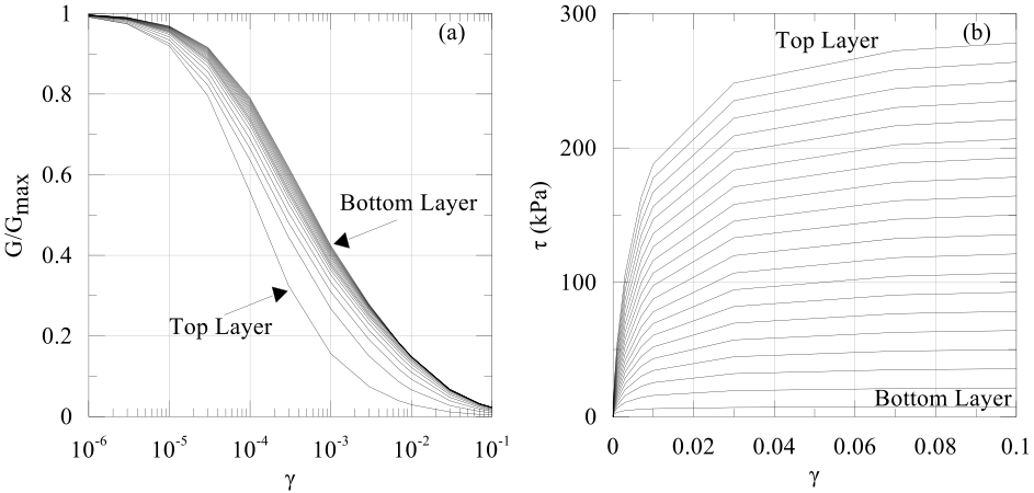
Figure 2: Modulus reduction and backbone curves (reprinted from Baltaji et al. 2017).

In this example, since the model does not exhibit a significant change in the mean effective stress during shaking, the pressure dependency parameters are set to be $ a_0 $ = 1, $ a_1 $ = 0, $ a_2 $ = 0, and $var element = document.getElementById("moose-equation-7d067dc3-4dd7-4766-8322-e0c09d161382");katex.render("b", element, {displayMode:false,throwOnError:false});$ = 0 so that the soil behavior is pressure independent.

Finally, the execution and output blocks are provided to run the analysis and extract the data using following chain of blocks (see Getting Started):

[Preconditioning<<<{"href": "../syntax/Preconditioning/index.html"}>>>]
  [./andy]
    type = SMP<<<{"description": "Single matrix preconditioner (SMP) builds a preconditioner using user defined off-diagonal parts of the Jacobian.", "href": "../source/preconditioners/SingleMatrixPreconditioner.html"}>>>
    full<<<{"description": "Set to true if you want the full set of couplings between variables simply for convenience so you don't have to set every off_diag_row and off_diag_column combination."}>>> = true
  [../]
[]

[Executioner<<<{"href": "../syntax/Executioner/index.html"}>>>]
  type = Transient
  solve_type = PJFNK
  nl_abs_tol = 1e-6
  nl_rel_tol = 1e-6
  l_tol = 1e-6
  l_max_its = 50
  start_time = 0.0
  end_time = 85.4
  dt = 0.005
  timestep_tolerance = 1e-6
  petsc_options = '-snes_ksp_ew'
  petsc_options_iname = '-ksp_gmres_restart -pc_type -pc_hypre_type -pc_hypre_boomeramg_max_iter'
  petsc_options_value = '201                hypre    boomeramg      4'
  line_search = 'none'
[]

[Postprocessors<<<{"href": "../syntax/Postprocessors/index.html"}>>>]
  [./accelx_top]
    type = PointValue<<<{"description": "Compute the value of a variable at a specified location", "href": "../source/postprocessors/PointValue.html"}>>>
    point<<<{"description": "The physical point where the solution will be evaluated."}>>> = '0.0 0.0 20.0'
    variable<<<{"description": "The name of the variable that this postprocessor operates on."}>>> = accel_x
  [../]
  [./accelx_top1]
    type = PointValue<<<{"description": "Compute the value of a variable at a specified location", "href": "../source/postprocessors/PointValue.html"}>>>
    point<<<{"description": "The physical point where the solution will be evaluated."}>>> = '0.0 0.0 19.0'
    variable<<<{"description": "The name of the variable that this postprocessor operates on."}>>> = accel_x
  [../]
  [./accelx_mid]
    type = PointValue<<<{"description": "Compute the value of a variable at a specified location", "href": "../source/postprocessors/PointValue.html"}>>>
    point<<<{"description": "The physical point where the solution will be evaluated."}>>> = '0.0 0.0 10.0'
    variable<<<{"description": "The name of the variable that this postprocessor operates on."}>>> = accel_x
  [../]
  [./accelx_bot]
    type = PointValue<<<{"description": "Compute the value of a variable at a specified location", "href": "../source/postprocessors/PointValue.html"}>>>
    point<<<{"description": "The physical point where the solution will be evaluated."}>>> = '0.0 0.0 0.0'
    variable<<<{"description": "The name of the variable that this postprocessor operates on."}>>> = accel_x
  [../]
[]

[VectorPostprocessors<<<{"href": "../syntax/VectorPostprocessors/index.html"}>>>]
  [./accel_hist]
    type = ResponseHistoryBuilder<<<{"description": "Calculates response histories for a given node and variable(s).", "href": "../source/vectorpostprocessors/ResponseHistoryBuilder.html"}>>>
    variables<<<{"description": "Variable name for which the response history is requested."}>>> = 'accel_x'
    nodes<<<{"description": "Node number(s) at which the response history is needed."}>>> = '80'
  [../]
  [./accel_spec]
    type = ResponseSpectraCalculator<<<{"description": "Calculate the response spectrum at the requested nodes or points.", "href": "../source/vectorpostprocessors/ResponseSpectraCalculator.html"}>>>
    vectorpostprocessor<<<{"description": "Name of the ResponseHistoryBuilder vectorpostprocessor, for which response spectra are calculated."}>>> = accel_hist
    regularize_dt<<<{"description": "dt for response spectra calculation. The acceleration response will be regularized to this dt prior to the response spectrum calculation."}>>> = 0.005
    outputs<<<{"description": "Vector of output names where you would like to restrict the output of variables(s) associated with this object"}>>> = out
  [../]
[]

[Outputs<<<{"href": "../syntax/Mastodon/Outputs/index.html"}>>>]
  csv<<<{"description": "Output the scalar variable and postprocessors to a *.csv file using the default CSV output."}>>> = true
  exodus<<<{"description": "Output the results using the default settings for Exodus output."}>>> = true
  perf_graph<<<{"description": "Enable printing of the performance graph to the screen (Console)"}>>> = true
  print_linear_residuals<<<{"description": "Enable printing of linear residuals to the screen (Console)"}>>> = true
  [./out]
   type = CSV<<<{"description": "Output for postprocessors, vector postprocessors, and scalar variables using comma seperated values (CSV).", "href": "../source/outputs/CSV.html"}>>>
   execute_on<<<{"description": "The list of flag(s) indicating when this object should be executed. For a description of each flag, see https://mooseframework.inl.gov/source/interfaces/SetupInterface.html."}>>> = 'timestep_begin'
   file_base<<<{"description": "The desired solution output name without an extension. If not provided, MOOSE sets it with Outputs/file_base when available. Otherwise, MOOSE uses input file name and this object name for a master input or uses master file_base, the subapp name and this object name for a subapp input to set it."}>>> = topsoil_response
  [../]
  [./screen]
   type = Console<<<{"description": "Object for screen output.", "href": "../source/outputs/Console.html"}>>>
   max_rows<<<{"description": "The maximum number of postprocessor/scalar values displayed on screen during a timestep (set to 0 for unlimited)"}>>> = 1
   interval = 1000
  [../]
[]

Accelerations obtained at the bottom, mid-depth and top of the soil columns are used to calculate the spectral response for 5 percent damping, the results are compared to analogous model developed in DEEPSOIL and presented in

Figure 3: Comparison of spectral accelerations from MASTODON and DEEPSOIL (modified from Baltaji et al. (2017)).

Further details regarding to application of MASTODON to simulate seismic site response and soil structure interaction analysis can be found in Baltaji et al. (2017).

Implementation using Automatic Differentiation

This example can also be run using Automatic Differentiation (AD). Automatic Differentiation enables the computation of a numerical Jacobian that is almost identical to the theoretical Jacobian of a kernel. This results in much quicker convergence, even for highly nonlinear problems. Therefore, solve_type=NEWTON can be used in the executioner, which uses the full Jacobian unlike solve_type=PJFNK, which is recommended when only an approximate estimate of the Jacobian is available. In MASTODON, the iSoil material model has been converted to AD and the usage of the AD version of iSoil is demonstrated below. More information can be found in ISoil material.

The following two modifications to the input file should be made to run this example using AD. These modifications ensure the AD versions of the stress divergence kernels and the material kernels are being used during the solve. Add 'use_automatic_differentiation = true' in 'Kernels/DynamicTensorMechanics':

[Kernels<<<{"href": "../syntax/Kernels/index.html"}>>>]
  [./DynamicTensorMechanics<<<{"href": "../syntax/Kernels/DynamicTensorMechanics/index.html"}>>>]
    displacements<<<{"description": "The nonlinear displacement variables for the problem"}>>> = 'disp_x disp_y disp_z'
    stiffness_damping_coefficient<<<{"description": "Name of material property or a constant real number defining stiffness Rayleigh parameter (zeta)."}>>> = 0.000781
    use_automatic_differentiation<<<{"description": "Flag to use automatic differentiation (AD) objects when possible"}>>> = true
  [../]
  [./inertia_x]
    type = InertialForce<<<{"description": "Calculates the residual for the inertial force ($M \\cdot acceleration$) and the contribution of mass dependent Rayleigh damping and HHT time  integration scheme ($\\eta \\cdot M \\cdot ((1+\\alpha)velq2-\\alpha \\cdot vel-old) $)", "href": "../source/kernels/InertialForce.html"}>>>
    variable<<<{"description": "The name of the variable that this residual object operates on"}>>> = disp_x
    velocity<<<{"description": "velocity variable"}>>> = vel_x
    acceleration<<<{"description": "acceleration variable"}>>> = accel_x
    beta<<<{"description": "beta parameter for Newmark Time integration"}>>> = 0.25
    gamma<<<{"description": "gamma parameter for Newmark Time integration"}>>> = 0.5
    eta<<<{"description": "Name of material property or a constant real number defining the eta parameter for the Rayleigh damping."}>>> = 0.64026
    density<<<{"description": "Name of Material Property that provides the density"}>>> = 'reg_density'
  [../]
  [./inertia_y]
    type = InertialForce<<<{"description": "Calculates the residual for the inertial force ($M \\cdot acceleration$) and the contribution of mass dependent Rayleigh damping and HHT time  integration scheme ($\\eta \\cdot M \\cdot ((1+\\alpha)velq2-\\alpha \\cdot vel-old) $)", "href": "../source/kernels/InertialForce.html"}>>>
    variable<<<{"description": "The name of the variable that this residual object operates on"}>>> = disp_y
    velocity<<<{"description": "velocity variable"}>>> = vel_y
    acceleration<<<{"description": "acceleration variable"}>>> = accel_y
    beta<<<{"description": "beta parameter for Newmark Time integration"}>>> = 0.25
    gamma<<<{"description": "gamma parameter for Newmark Time integration"}>>> = 0.5
    eta<<<{"description": "Name of material property or a constant real number defining the eta parameter for the Rayleigh damping."}>>> = 0.64026
    density<<<{"description": "Name of Material Property that provides the density"}>>> = 'reg_density'
  [../]
  [./inertia_z]
    type = InertialForce<<<{"description": "Calculates the residual for the inertial force ($M \\cdot acceleration$) and the contribution of mass dependent Rayleigh damping and HHT time  integration scheme ($\\eta \\cdot M \\cdot ((1+\\alpha)velq2-\\alpha \\cdot vel-old) $)", "href": "../source/kernels/InertialForce.html"}>>>
    variable<<<{"description": "The name of the variable that this residual object operates on"}>>> = disp_z
    velocity<<<{"description": "velocity variable"}>>> = vel_z
    acceleration<<<{"description": "acceleration variable"}>>> = accel_z
    beta<<<{"description": "beta parameter for Newmark Time integration"}>>> = 0.25
    gamma<<<{"description": "gamma parameter for Newmark Time integration"}>>> = 0.5
    eta<<<{"description": "Name of material property or a constant real number defining the eta parameter for the Rayleigh damping."}>>> = 0.64026
    density<<<{"description": "Name of Material Property that provides the density"}>>> = 'reg_density'
  [../]
  [./gravity]
    type = Gravity<<<{"description": "Apply gravity. Value is in units of acceleration.", "href": "../source/kernels/Gravity.html"}>>>
    variable<<<{"description": "The name of the variable that this residual object operates on"}>>> = disp_z
    value<<<{"description": "Value multiplied against the residual, e.g. gravitational acceleration"}>>> = -9.81
    density<<<{"description": "The density"}>>> = 'reg_density'
  [../]
[]

Also, add 'use_automatic_differentiation = true' in 'Materials/I_Soil/soil_all':

[Materials<<<{"href": "../syntax/Materials/index.html"}>>>]
  [./I_Soil<<<{"href": "../syntax/Materials/I_Soil/index.html"}>>>]
    [./soil_all]
       block<<<{"description": "The blocks where this material model is applied."}>>> = 0
       layer_variable<<<{"description": "The auxvariable providing the soil layer identification."}>>> = layer_id
       layer_ids<<<{"description": "Vector of layer ids that map one-to-one to the rest of the soil layer parameters provided as input."}>>> = '0 1 2 3 4 5 6 7 8 9 10 11 12 13 14 15 16 17 18 19'
       initial_soil_stress<<<{"description": "The function values for the initial stress distribution. 9 function names have to be provided corresponding to stress_xx, stress_xy, stress_xz, stress_yx, stress_yy, stress_yz, stress_zx, stress_zy, stress_zz. Each function can be a function of space."}>>> = 'initial_xx 0 0 0 initial_xx 0 0 0 initial_zz'
       poissons_ratio<<<{"description": "Poissons's ratio for the soil layers. The size of the vector should be same as the size of layer_ids."}>>> = '0.3 0.3 0.3 0.3 0.3 0.3 0.3 0.3 0.3 0.3 0.3 0.3 0.3 0.3 0.3 0.3 0.3 0.3 0.3 0.3'
       soil_type<<<{"description": "This parameter determines the type of backbone curve used. Use 'user_defined' for a user defined backbone curve provided in a data file, 'darendeli' if the backbone curve is to be determined using Darandeli equations, 'gqh' if the backbone curve is determined using the GQ/H approach and 'thin_layer' if the soil is being used to simulate a thin-layer friction interface."}>>> = 'gqh'
       number_of_points<<<{"description": "The total number of data points in which the backbone curve needs to be split for all soil layers (required for Darandeli or GQ/H type backbone curves)."}>>> = 100
       ### GQ/H ####
       initial_shear_modulus<<<{"description": "The initial shear modulus of the soil layers."}>>> = '125000000 118098000 111392000 103968000 96800000 89888000 83232000 76832000 70688000 64800000 59168000 53792000 48672000 43808000 39200000 34848000 30752000 26912000 23328000 20000000'
       theta_1<<<{"description": "The curve fit coefficient for GQ/H modelfor each soil layer."}>>> = '-6.66 -6.86 -7.06 -7.35 -7.65 -7.95 -8.3 -8.61 -8.95 -9.3 -9.61 -9.92 -10.0 -10.0 -10.0 -10.0 -10.0 -9.31 -7.17 -5.54'
       theta_2<<<{"description": "The curve fit coefficient for GQ/H modelfor each soil layer."}>>> = '5.5 5.7 5.9 6.2 6.6 6.9 7.3 7.6 8.0 8.4 8.6 8.8 8.82 8.71 8.55 8.3 7.88 6.4 2.4 -2.28'
       theta_3<<<{"description": "The curve fit coefficient for GQ/H modelfor each soil layer."}>>> = '1.0 1.0 1.0 1.0 1.0 1.0 1.0 1.0 1.0 1.0 1.0 1.0 1.0 1.0 1.0 1.0 1.0 1.0 1.0 1.0'
       theta_4<<<{"description": "The curve fit coefficient for GQ/H modelfor each soil layer."}>>> = '1.0 1.0 1.0 1.0 1.0 1.0 1.0 1.0 1.0 1.0 1.0 1.0 1.0 1.0 1.0 1.0 1.0 1.0 1.0 1.0'
       theta_5<<<{"description": "The curve fit coefficient for GQ/H modelfor each soil layer."}>>> = '0.99 0.99 0.99 0.99 0.99 0.99 0.99 0.99 0.99 0.99 0.99 0.99 0.99 0.99 0.99 0.99 0.99 0.99 0.99 0.99'
       taumax<<<{"description": "The ultimate shear strength of the soil layers. Required for GQ/H model"}>>> = '292500 277500 262500 247500 232500 217500 202500 187500 172500 157500 142500 127500 112500 97500 82500 67500 52500 37500 22500 7500'
       p_ref<<<{"description": "The reference pressure at which the parameters are defined for each soil layer. If 'soil_type = darendeli', then the reference pressure must be input in kilopascals."}>>> = '236841 224695 212550 200404 188258 176112 163967 151821 139675 127530 115384 103238 91092 78947 66801 54655 42510 30364 18218 6072'
       ######
       density<<<{"description": "Vector of density values that map one-to-one with the number 'layer_ids' parameter."}>>> = '2000.0 2000.0 2000.0 2000.0 2000.0 2000.0 2000.0 2000.0 2000.0 2000.0 2000.0 2000.0 2000.0 2000.0 2000.0 2000.0 2000.0 2000.0 2000.0 2000.0'
       a0<<<{"description": "The first coefficient for pressure dependent yield strength calculation for all the soil layers. If a0 = 1, a1 = 0 and a2=0 for one soil layer, then the yield strength of that layer is independent of pressure."}>>> = 1.0
       a1<<<{"description": "The second coefficient for pressure dependent yield strength calculation for all the soil layers. If a0 = 1, a1 = 0, a2 = 0 for one soil layer, then the yield strength of that layer is independent of pressure."}>>> = 0.0
       a2<<<{"description": "The third coefficient for pressure dependent yield strength calculation for all the soil layers. If a0 = 1, a1=0 and a2=0 for one soil layer, then the yield strength of that layer is independent of pressure."}>>> = 0.0
       b_exp<<<{"description": "The exponential factors for pressure dependent stiffness for all the soil layers."}>>> = 0.0
       use_automatic_differentiation<<<{"description": "Flag to use automatic differentiation (AD) objects when possible"}>>> = true
    [../]
  [../]
  [converter]
    type = MaterialConverter<<<{"description": "Converts regular material properties to AD properties and vice versa", "href": "../source/materials/MaterialADConverter.html"}>>>
    ad_props_in<<<{"description": "The names of the AD material properties to convert to regular properties"}>>> = 'density'
    reg_props_out<<<{"description": "The names of the output regular properties"}>>> = 'reg_density'
  []
[]

The plots below present the accelerations and response spectra at the top soil computed using AD and no-AD. The AD and the no-AD results quite closely match.

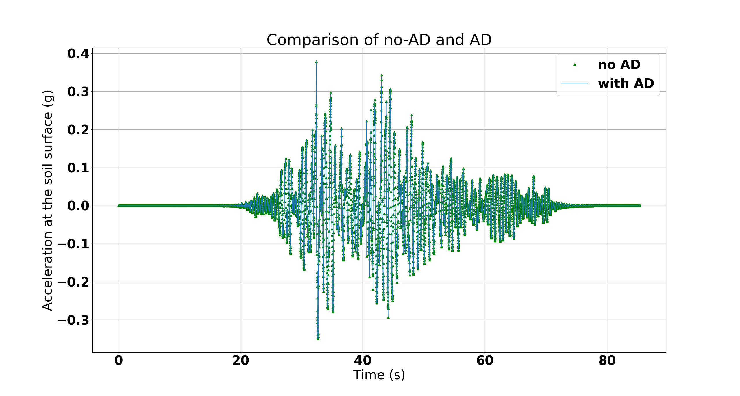
Figure 4: Comparison of accelerations at the soil surface generated using AD and no-AD.

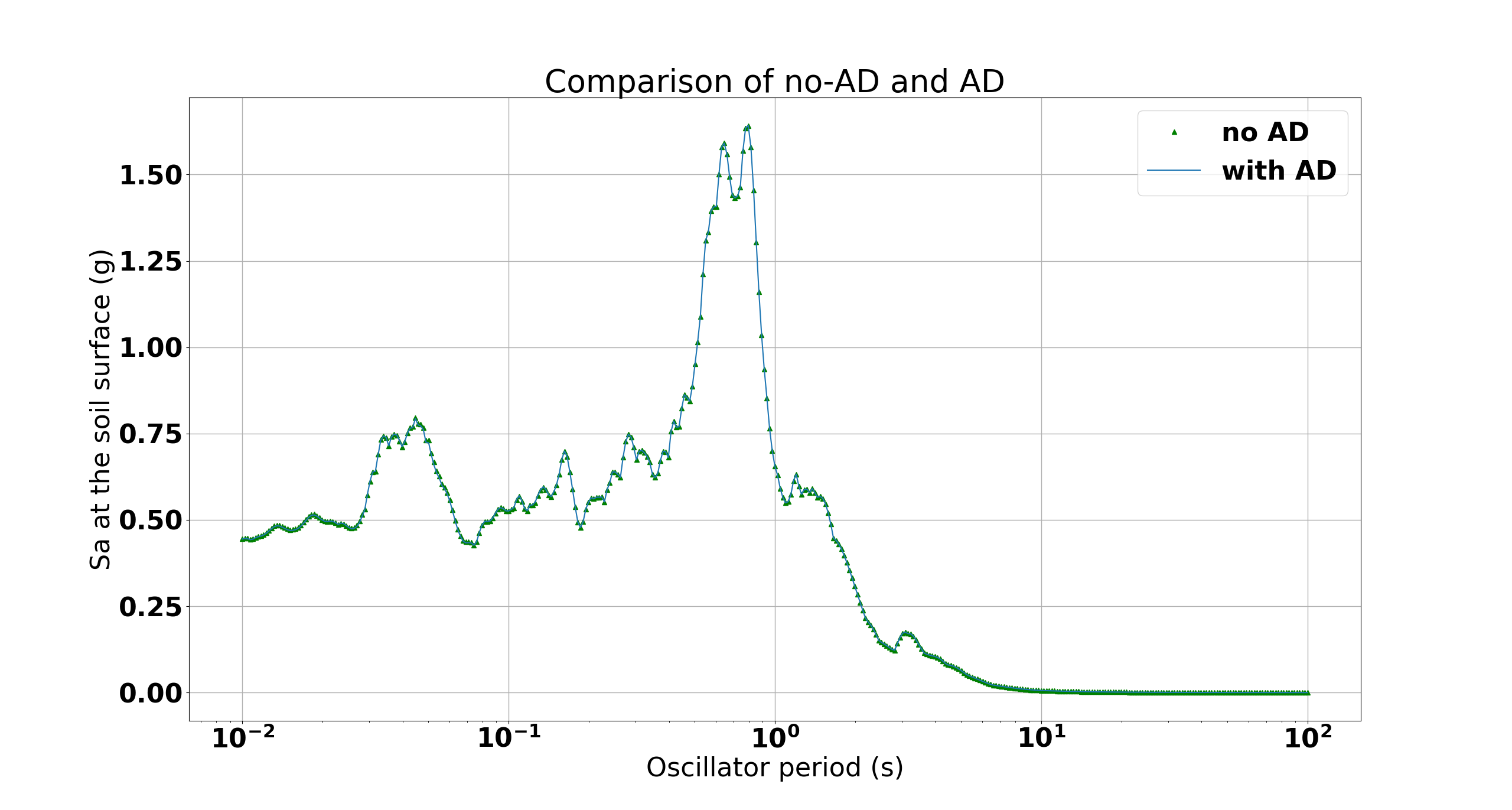
Figure 5: Comparison of response spectra at the soil surface generated using AD and no-AD.

References

O. Baltaji, O. Numanoglu, S. Veeraraghavan, Y. M. A. Hashash, J. L. Coleman, and C. Bolisetti. Non-linear time domain site response and soil structure analysis for nuclear facilities using MOOSE. Transactions, 24th International Conference on Structural Mechanics in Reactor Technology (SMiRT 24), Busan, South Korea, August 2017., 2017.

@article{baltaji2017nonlinear,
    author = "Baltaji, O. and Numanoglu, O. and Veeraraghavan, S. and Hashash, Y. M. A. and Coleman, J. L. and Bolisetti, C.",
    title = "Non-linear time domain site response and soil structure analysis for nuclear facilities using {MOOSE}",
    journal = "Transactions, 24th International Conference on Structural Mechanics in Reactor Technology (SMiRT 24), Busan, South Korea, August 2017.",
    year = "2017"
}

(examples/ex03a/shear_beam_Isoil_free_field.i)

[Mesh]
  type = GeneratedMesh
  nx = 1
  ny = 1
  nz = 20
  xmin = -0.5
  ymin = -0.5
  zmin = 0.0
  xmax = 0.5
  ymax = 0.5
  zmax = 20.0
  dim = 3
[]

[GlobalParams]
  displacements = 'disp_x disp_y disp_z'
[]

[Variables]
  [./disp_x]
  [../]
  [./disp_y]
  [../]
  [./disp_z]
  [../]
[]

[AuxVariables]
  [./vel_x]
  [../]
  [./accel_x]
  [../]
  [./vel_y]
  [../]
  [./accel_y]
  [../]
  [./vel_z]
  [../]
  [./accel_z]
  [../]
  [./layer_id]
    order = CONSTANT
    family = MONOMIAL
  [../]
[]

[Kernels]
  [./DynamicTensorMechanics]
    displacements = 'disp_x disp_y disp_z'
    stiffness_damping_coefficient = 0.000781
  [../]
  [./inertia_x]
    type = InertialForce
    variable = disp_x
    velocity = vel_x
    acceleration = accel_x
    beta = 0.25
    gamma = 0.5
    eta = 0.64026
  [../]
  [./inertia_y]
    type = InertialForce
    variable = disp_y
    velocity = vel_y
    acceleration = accel_y
    beta = 0.25
    gamma = 0.5
    eta = 0.64026
  [../]
  [./inertia_z]
    type = InertialForce
    variable = disp_z
    velocity = vel_z
    acceleration = accel_z
    beta = 0.25
    gamma = 0.5
    eta = 0.64026
  [../]
  [./gravity]
    type = Gravity
    variable = disp_z
    value = -9.81
  [../]
[]

[AuxKernels]
  [./accel_x]
    type = NewmarkAccelAux
    variable = accel_x
    displacement = disp_x
    velocity = vel_x
    beta = 0.25
    execute_on = timestep_end
  [../]
  [./vel_x]
    type = NewmarkVelAux
    variable = vel_x
    acceleration = accel_x
    gamma = 0.5
    execute_on = timestep_end
  [../]
  [./accel_y]
    type = NewmarkAccelAux
    variable = accel_y
    displacement = disp_y
    velocity = vel_y
    beta = 0.25
    execute_on = timestep_end
  [../]
  [./vel_y]
    type = NewmarkVelAux
    variable = vel_y
    acceleration = accel_y
    gamma = 0.5
    execute_on = timestep_end
  [../]
  [./accel_z]
    type = NewmarkAccelAux
    variable = accel_z
    displacement = disp_z
    velocity = vel_z
    beta = 0.25
    execute_on = timestep_end
  [../]
  [./vel_z]
    type = NewmarkVelAux
    variable = vel_z
    acceleration = accel_z
    gamma = 0.5
    execute_on = timestep_end
  [../]
  [./layer_id]
     type = UniformLayerAuxKernel
     variable = layer_id
     interfaces = '1 2 3 4 5 6 7 8 9 10 11 12 13 14 15 16 17 18 19 20.2'
     direction = '0.0 0.0 1.0'
     execute_on = initial
  [../]
[]

[BCs]
  [./bottom_z]
    type = DirichletBC
    variable = disp_z
    boundary = 'back'
    value = 0.0
  [../]
  [./bottom_y]
    type = DirichletBC
    variable = disp_y
    boundary = 'back'
    value = 0.0
  [../]
  [./bottom_accel]
    type = PresetAcceleration
    boundary = 'back'
    function = accel_bottom
    variable = 'disp_x'
    beta = 0.25
    acceleration = 'accel_x'
    velocity = 'vel_x'
  [../]
  [./Periodic]
    [./y_dir]
      variable = 'disp_x disp_y disp_z'
      primary = 'bottom'
      secondary = 'top'
      translation = '0.0 1.0 0.0'
    [../]
    [./x_dir]
      variable = 'disp_x disp_y disp_z'
      primary = 'left'
      secondary = 'right'
      translation = '1.0 0.0 0.0'
    [../]
  [../]
[]

[Functions]
  [./accel_bottom]
     type = PiecewiseLinear
     data_file = chichi_bc_mpss_xp20.csv
     format = 'columns'
  [../]
  [./initial_zz]
    type = ParsedFunction
    value = '-2000.0 * 9.81 * (20.0 - z)'
  [../]
  [./initial_xx]
    type = ParsedFunction
    value = '-2000.0 * 9.81 * (20.0 - z) * 0.3/0.7'
  [../]
[]

[Materials]
  [./I_Soil]
    [./soil_all]
       block = 0
       layer_variable = layer_id
       layer_ids = '0 1 2 3 4 5 6 7 8 9 10 11 12 13 14 15 16 17 18 19'
       initial_soil_stress = 'initial_xx 0 0 0 initial_xx 0 0 0 initial_zz'
       poissons_ratio = '0.3 0.3 0.3 0.3 0.3 0.3 0.3 0.3 0.3 0.3 0.3 0.3 0.3 0.3 0.3 0.3 0.3 0.3 0.3 0.3'
       soil_type = 'gqh'
       number_of_points = 100
       ### GQ/H ####
       initial_shear_modulus = '125000000 118098000 111392000 103968000 96800000 89888000 83232000 76832000 70688000 64800000 59168000 53792000 48672000 43808000 39200000 34848000 30752000 26912000 23328000 20000000'
       theta_1 = '-6.66 -6.86 -7.06 -7.35 -7.65 -7.95 -8.3 -8.61 -8.95 -9.3 -9.61 -9.92 -10.0 -10.0 -10.0 -10.0 -10.0 -9.31 -7.17 -5.54'
       theta_2 = '5.5 5.7 5.9 6.2 6.6 6.9 7.3 7.6 8.0 8.4 8.6 8.8 8.82 8.71 8.55 8.3 7.88 6.4 2.4 -2.28'
       theta_3 = '1.0 1.0 1.0 1.0 1.0 1.0 1.0 1.0 1.0 1.0 1.0 1.0 1.0 1.0 1.0 1.0 1.0 1.0 1.0 1.0'
       theta_4 = '1.0 1.0 1.0 1.0 1.0 1.0 1.0 1.0 1.0 1.0 1.0 1.0 1.0 1.0 1.0 1.0 1.0 1.0 1.0 1.0'
       theta_5 = '0.99 0.99 0.99 0.99 0.99 0.99 0.99 0.99 0.99 0.99 0.99 0.99 0.99 0.99 0.99 0.99 0.99 0.99 0.99 0.99'
       taumax = '292500 277500 262500 247500 232500 217500 202500 187500 172500 157500 142500 127500 112500 97500 82500 67500 52500 37500 22500 7500'
       p_ref = '236841 224695 212550 200404 188258 176112 163967 151821 139675 127530 115384 103238 91092 78947 66801 54655 42510 30364 18218 6072'
       ######
       density = '2000.0 2000.0 2000.0 2000.0 2000.0 2000.0 2000.0 2000.0 2000.0 2000.0 2000.0 2000.0 2000.0 2000.0 2000.0 2000.0 2000.0 2000.0 2000.0 2000.0'
       a0 = 1.0
       a1 = 0.0
       a2 = 0.0
       b_exp = 0.0
    [../]
  [../]
[]

[Preconditioning]
  [./andy]
    type = SMP
    full = true
  [../]
[]

[Executioner]
  type = Transient
  solve_type = PJFNK
  nl_abs_tol = 1e-6
  nl_rel_tol = 1e-6
  l_tol = 1e-6
  l_max_its = 50
  start_time = 0.0
  end_time = 85.4
  dt = 0.005
  timestep_tolerance = 1e-6
  petsc_options = '-snes_ksp_ew'
  petsc_options_iname = '-ksp_gmres_restart -pc_type -pc_hypre_type -pc_hypre_boomeramg_max_iter'
  petsc_options_value = '201                hypre    boomeramg      4'
  line_search = 'none'
[]

[Postprocessors]
  [./accelx_top]
    type = PointValue
    point = '0.0 0.0 20.0'
    variable = accel_x
  [../]
  [./accelx_top1]
    type = PointValue
    point = '0.0 0.0 19.0'
    variable = accel_x
  [../]
  [./accelx_mid]
    type = PointValue
    point = '0.0 0.0 10.0'
    variable = accel_x
  [../]
  [./accelx_bot]
    type = PointValue
    point = '0.0 0.0 0.0'
    variable = accel_x
  [../]
[]

[VectorPostprocessors]
  [./accel_hist]
    type = ResponseHistoryBuilder
    variables = 'accel_x'
    nodes = '80'
  [../]
  [./accel_spec]
    type = ResponseSpectraCalculator
    vectorpostprocessor = accel_hist
    regularize_dt = 0.005
    outputs = out
  [../]
[]

[Outputs]
  csv = true
  exodus = true
  perf_graph = true
  print_linear_residuals = true
  [./out]
   type = CSV
   execute_on = 'timestep_begin'
   file_base = topsoil_response
  [../]
  [./screen]
   type = Console
   max_rows = 1
   interval = 1000
  [../]
[]

(examples/ex03a/shear_beam_Isoil_free_field.i)

[Mesh]
  type = GeneratedMesh
  nx = 1
  ny = 1
  nz = 20
  xmin = -0.5
  ymin = -0.5
  zmin = 0.0
  xmax = 0.5
  ymax = 0.5
  zmax = 20.0
  dim = 3
[]

[GlobalParams]
  displacements = 'disp_x disp_y disp_z'
[]

[Variables]
  [./disp_x]
  [../]
  [./disp_y]
  [../]
  [./disp_z]
  [../]
[]

[AuxVariables]
  [./vel_x]
  [../]
  [./accel_x]
  [../]
  [./vel_y]
  [../]
  [./accel_y]
  [../]
  [./vel_z]
  [../]
  [./accel_z]
  [../]
  [./layer_id]
    order = CONSTANT
    family = MONOMIAL
  [../]
[]

[Kernels]
  [./DynamicTensorMechanics]
    displacements = 'disp_x disp_y disp_z'
    stiffness_damping_coefficient = 0.000781
  [../]
  [./inertia_x]
    type = InertialForce
    variable = disp_x
    velocity = vel_x
    acceleration = accel_x
    beta = 0.25
    gamma = 0.5
    eta = 0.64026
  [../]
  [./inertia_y]
    type = InertialForce
    variable = disp_y
    velocity = vel_y
    acceleration = accel_y
    beta = 0.25
    gamma = 0.5
    eta = 0.64026
  [../]
  [./inertia_z]
    type = InertialForce
    variable = disp_z
    velocity = vel_z
    acceleration = accel_z
    beta = 0.25
    gamma = 0.5
    eta = 0.64026
  [../]
  [./gravity]
    type = Gravity
    variable = disp_z
    value = -9.81
  [../]
[]

[AuxKernels]
  [./accel_x]
    type = NewmarkAccelAux
    variable = accel_x
    displacement = disp_x
    velocity = vel_x
    beta = 0.25
    execute_on = timestep_end
  [../]
  [./vel_x]
    type = NewmarkVelAux
    variable = vel_x
    acceleration = accel_x
    gamma = 0.5
    execute_on = timestep_end
  [../]
  [./accel_y]
    type = NewmarkAccelAux
    variable = accel_y
    displacement = disp_y
    velocity = vel_y
    beta = 0.25
    execute_on = timestep_end
  [../]
  [./vel_y]
    type = NewmarkVelAux
    variable = vel_y
    acceleration = accel_y
    gamma = 0.5
    execute_on = timestep_end
  [../]
  [./accel_z]
    type = NewmarkAccelAux
    variable = accel_z
    displacement = disp_z
    velocity = vel_z
    beta = 0.25
    execute_on = timestep_end
  [../]
  [./vel_z]
    type = NewmarkVelAux
    variable = vel_z
    acceleration = accel_z
    gamma = 0.5
    execute_on = timestep_end
  [../]
  [./layer_id]
     type = UniformLayerAuxKernel
     variable = layer_id
     interfaces = '1 2 3 4 5 6 7 8 9 10 11 12 13 14 15 16 17 18 19 20.2'
     direction = '0.0 0.0 1.0'
     execute_on = initial
  [../]
[]

[BCs]
  [./bottom_z]
    type = DirichletBC
    variable = disp_z
    boundary = 'back'
    value = 0.0
  [../]
  [./bottom_y]
    type = DirichletBC
    variable = disp_y
    boundary = 'back'
    value = 0.0
  [../]
  [./bottom_accel]
    type = PresetAcceleration
    boundary = 'back'
    function = accel_bottom
    variable = 'disp_x'
    beta = 0.25
    acceleration = 'accel_x'
    velocity = 'vel_x'
  [../]
  [./Periodic]
    [./y_dir]
      variable = 'disp_x disp_y disp_z'
      primary = 'bottom'
      secondary = 'top'
      translation = '0.0 1.0 0.0'
    [../]
    [./x_dir]
      variable = 'disp_x disp_y disp_z'
      primary = 'left'
      secondary = 'right'
      translation = '1.0 0.0 0.0'
    [../]
  [../]
[]

[Functions]
  [./accel_bottom]
     type = PiecewiseLinear
     data_file = chichi_bc_mpss_xp20.csv
     format = 'columns'
  [../]
  [./initial_zz]
    type = ParsedFunction
    value = '-2000.0 * 9.81 * (20.0 - z)'
  [../]
  [./initial_xx]
    type = ParsedFunction
    value = '-2000.0 * 9.81 * (20.0 - z) * 0.3/0.7'
  [../]
[]

[Materials]
  [./I_Soil]
    [./soil_all]
       block = 0
       layer_variable = layer_id
       layer_ids = '0 1 2 3 4 5 6 7 8 9 10 11 12 13 14 15 16 17 18 19'
       initial_soil_stress = 'initial_xx 0 0 0 initial_xx 0 0 0 initial_zz'
       poissons_ratio = '0.3 0.3 0.3 0.3 0.3 0.3 0.3 0.3 0.3 0.3 0.3 0.3 0.3 0.3 0.3 0.3 0.3 0.3 0.3 0.3'
       soil_type = 'gqh'
       number_of_points = 100
       ### GQ/H ####
       initial_shear_modulus = '125000000 118098000 111392000 103968000 96800000 89888000 83232000 76832000 70688000 64800000 59168000 53792000 48672000 43808000 39200000 34848000 30752000 26912000 23328000 20000000'
       theta_1 = '-6.66 -6.86 -7.06 -7.35 -7.65 -7.95 -8.3 -8.61 -8.95 -9.3 -9.61 -9.92 -10.0 -10.0 -10.0 -10.0 -10.0 -9.31 -7.17 -5.54'
       theta_2 = '5.5 5.7 5.9 6.2 6.6 6.9 7.3 7.6 8.0 8.4 8.6 8.8 8.82 8.71 8.55 8.3 7.88 6.4 2.4 -2.28'
       theta_3 = '1.0 1.0 1.0 1.0 1.0 1.0 1.0 1.0 1.0 1.0 1.0 1.0 1.0 1.0 1.0 1.0 1.0 1.0 1.0 1.0'
       theta_4 = '1.0 1.0 1.0 1.0 1.0 1.0 1.0 1.0 1.0 1.0 1.0 1.0 1.0 1.0 1.0 1.0 1.0 1.0 1.0 1.0'
       theta_5 = '0.99 0.99 0.99 0.99 0.99 0.99 0.99 0.99 0.99 0.99 0.99 0.99 0.99 0.99 0.99 0.99 0.99 0.99 0.99 0.99'
       taumax = '292500 277500 262500 247500 232500 217500 202500 187500 172500 157500 142500 127500 112500 97500 82500 67500 52500 37500 22500 7500'
       p_ref = '236841 224695 212550 200404 188258 176112 163967 151821 139675 127530 115384 103238 91092 78947 66801 54655 42510 30364 18218 6072'
       ######
       density = '2000.0 2000.0 2000.0 2000.0 2000.0 2000.0 2000.0 2000.0 2000.0 2000.0 2000.0 2000.0 2000.0 2000.0 2000.0 2000.0 2000.0 2000.0 2000.0 2000.0'
       a0 = 1.0
       a1 = 0.0
       a2 = 0.0
       b_exp = 0.0
    [../]
  [../]
[]

[Preconditioning]
  [./andy]
    type = SMP
    full = true
  [../]
[]

[Executioner]
  type = Transient
  solve_type = PJFNK
  nl_abs_tol = 1e-6
  nl_rel_tol = 1e-6
  l_tol = 1e-6
  l_max_its = 50
  start_time = 0.0
  end_time = 85.4
  dt = 0.005
  timestep_tolerance = 1e-6
  petsc_options = '-snes_ksp_ew'
  petsc_options_iname = '-ksp_gmres_restart -pc_type -pc_hypre_type -pc_hypre_boomeramg_max_iter'
  petsc_options_value = '201                hypre    boomeramg      4'
  line_search = 'none'
[]

[Postprocessors]
  [./accelx_top]
    type = PointValue
    point = '0.0 0.0 20.0'
    variable = accel_x
  [../]
  [./accelx_top1]
    type = PointValue
    point = '0.0 0.0 19.0'
    variable = accel_x
  [../]
  [./accelx_mid]
    type = PointValue
    point = '0.0 0.0 10.0'
    variable = accel_x
  [../]
  [./accelx_bot]
    type = PointValue
    point = '0.0 0.0 0.0'
    variable = accel_x
  [../]
[]

[VectorPostprocessors]
  [./accel_hist]
    type = ResponseHistoryBuilder
    variables = 'accel_x'
    nodes = '80'
  [../]
  [./accel_spec]
    type = ResponseSpectraCalculator
    vectorpostprocessor = accel_hist
    regularize_dt = 0.005
    outputs = out
  [../]
[]

[Outputs]
  csv = true
  exodus = true
  perf_graph = true
  print_linear_residuals = true
  [./out]
   type = CSV
   execute_on = 'timestep_begin'
   file_base = topsoil_response
  [../]
  [./screen]
   type = Console
   max_rows = 1
   interval = 1000
  [../]
[]

(examples/ex03a/shear_beam_Isoil_free_field.i)

[Mesh]
  type = GeneratedMesh
  nx = 1
  ny = 1
  nz = 20
  xmin = -0.5
  ymin = -0.5
  zmin = 0.0
  xmax = 0.5
  ymax = 0.5
  zmax = 20.0
  dim = 3
[]

[GlobalParams]
  displacements = 'disp_x disp_y disp_z'
[]

[Variables]
  [./disp_x]
  [../]
  [./disp_y]
  [../]
  [./disp_z]
  [../]
[]

[AuxVariables]
  [./vel_x]
  [../]
  [./accel_x]
  [../]
  [./vel_y]
  [../]
  [./accel_y]
  [../]
  [./vel_z]
  [../]
  [./accel_z]
  [../]
  [./layer_id]
    order = CONSTANT
    family = MONOMIAL
  [../]
[]

[Kernels]
  [./DynamicTensorMechanics]
    displacements = 'disp_x disp_y disp_z'
    stiffness_damping_coefficient = 0.000781
  [../]
  [./inertia_x]
    type = InertialForce
    variable = disp_x
    velocity = vel_x
    acceleration = accel_x
    beta = 0.25
    gamma = 0.5
    eta = 0.64026
  [../]
  [./inertia_y]
    type = InertialForce
    variable = disp_y
    velocity = vel_y
    acceleration = accel_y
    beta = 0.25
    gamma = 0.5
    eta = 0.64026
  [../]
  [./inertia_z]
    type = InertialForce
    variable = disp_z
    velocity = vel_z
    acceleration = accel_z
    beta = 0.25
    gamma = 0.5
    eta = 0.64026
  [../]
  [./gravity]
    type = Gravity
    variable = disp_z
    value = -9.81
  [../]
[]

[AuxKernels]
  [./accel_x]
    type = NewmarkAccelAux
    variable = accel_x
    displacement = disp_x
    velocity = vel_x
    beta = 0.25
    execute_on = timestep_end
  [../]
  [./vel_x]
    type = NewmarkVelAux
    variable = vel_x
    acceleration = accel_x
    gamma = 0.5
    execute_on = timestep_end
  [../]
  [./accel_y]
    type = NewmarkAccelAux
    variable = accel_y
    displacement = disp_y
    velocity = vel_y
    beta = 0.25
    execute_on = timestep_end
  [../]
  [./vel_y]
    type = NewmarkVelAux
    variable = vel_y
    acceleration = accel_y
    gamma = 0.5
    execute_on = timestep_end
  [../]
  [./accel_z]
    type = NewmarkAccelAux
    variable = accel_z
    displacement = disp_z
    velocity = vel_z
    beta = 0.25
    execute_on = timestep_end
  [../]
  [./vel_z]
    type = NewmarkVelAux
    variable = vel_z
    acceleration = accel_z
    gamma = 0.5
    execute_on = timestep_end
  [../]
  [./layer_id]
     type = UniformLayerAuxKernel
     variable = layer_id
     interfaces = '1 2 3 4 5 6 7 8 9 10 11 12 13 14 15 16 17 18 19 20.2'
     direction = '0.0 0.0 1.0'
     execute_on = initial
  [../]
[]

[BCs]
  [./bottom_z]
    type = DirichletBC
    variable = disp_z
    boundary = 'back'
    value = 0.0
  [../]
  [./bottom_y]
    type = DirichletBC
    variable = disp_y
    boundary = 'back'
    value = 0.0
  [../]
  [./bottom_accel]
    type = PresetAcceleration
    boundary = 'back'
    function = accel_bottom
    variable = 'disp_x'
    beta = 0.25
    acceleration = 'accel_x'
    velocity = 'vel_x'
  [../]
  [./Periodic]
    [./y_dir]
      variable = 'disp_x disp_y disp_z'
      primary = 'bottom'
      secondary = 'top'
      translation = '0.0 1.0 0.0'
    [../]
    [./x_dir]
      variable = 'disp_x disp_y disp_z'
      primary = 'left'
      secondary = 'right'
      translation = '1.0 0.0 0.0'
    [../]
  [../]
[]

[Functions]
  [./accel_bottom]
     type = PiecewiseLinear
     data_file = chichi_bc_mpss_xp20.csv
     format = 'columns'
  [../]
  [./initial_zz]
    type = ParsedFunction
    value = '-2000.0 * 9.81 * (20.0 - z)'
  [../]
  [./initial_xx]
    type = ParsedFunction
    value = '-2000.0 * 9.81 * (20.0 - z) * 0.3/0.7'
  [../]
[]

[Materials]
  [./I_Soil]
    [./soil_all]
       block = 0
       layer_variable = layer_id
       layer_ids = '0 1 2 3 4 5 6 7 8 9 10 11 12 13 14 15 16 17 18 19'
       initial_soil_stress = 'initial_xx 0 0 0 initial_xx 0 0 0 initial_zz'
       poissons_ratio = '0.3 0.3 0.3 0.3 0.3 0.3 0.3 0.3 0.3 0.3 0.3 0.3 0.3 0.3 0.3 0.3 0.3 0.3 0.3 0.3'
       soil_type = 'gqh'
       number_of_points = 100
       ### GQ/H ####
       initial_shear_modulus = '125000000 118098000 111392000 103968000 96800000 89888000 83232000 76832000 70688000 64800000 59168000 53792000 48672000 43808000 39200000 34848000 30752000 26912000 23328000 20000000'
       theta_1 = '-6.66 -6.86 -7.06 -7.35 -7.65 -7.95 -8.3 -8.61 -8.95 -9.3 -9.61 -9.92 -10.0 -10.0 -10.0 -10.0 -10.0 -9.31 -7.17 -5.54'
       theta_2 = '5.5 5.7 5.9 6.2 6.6 6.9 7.3 7.6 8.0 8.4 8.6 8.8 8.82 8.71 8.55 8.3 7.88 6.4 2.4 -2.28'
       theta_3 = '1.0 1.0 1.0 1.0 1.0 1.0 1.0 1.0 1.0 1.0 1.0 1.0 1.0 1.0 1.0 1.0 1.0 1.0 1.0 1.0'
       theta_4 = '1.0 1.0 1.0 1.0 1.0 1.0 1.0 1.0 1.0 1.0 1.0 1.0 1.0 1.0 1.0 1.0 1.0 1.0 1.0 1.0'
       theta_5 = '0.99 0.99 0.99 0.99 0.99 0.99 0.99 0.99 0.99 0.99 0.99 0.99 0.99 0.99 0.99 0.99 0.99 0.99 0.99 0.99'
       taumax = '292500 277500 262500 247500 232500 217500 202500 187500 172500 157500 142500 127500 112500 97500 82500 67500 52500 37500 22500 7500'
       p_ref = '236841 224695 212550 200404 188258 176112 163967 151821 139675 127530 115384 103238 91092 78947 66801 54655 42510 30364 18218 6072'
       ######
       density = '2000.0 2000.0 2000.0 2000.0 2000.0 2000.0 2000.0 2000.0 2000.0 2000.0 2000.0 2000.0 2000.0 2000.0 2000.0 2000.0 2000.0 2000.0 2000.0 2000.0'
       a0 = 1.0
       a1 = 0.0
       a2 = 0.0
       b_exp = 0.0
    [../]
  [../]
[]

[Preconditioning]
  [./andy]
    type = SMP
    full = true
  [../]
[]

[Executioner]
  type = Transient
  solve_type = PJFNK
  nl_abs_tol = 1e-6
  nl_rel_tol = 1e-6
  l_tol = 1e-6
  l_max_its = 50
  start_time = 0.0
  end_time = 85.4
  dt = 0.005
  timestep_tolerance = 1e-6
  petsc_options = '-snes_ksp_ew'
  petsc_options_iname = '-ksp_gmres_restart -pc_type -pc_hypre_type -pc_hypre_boomeramg_max_iter'
  petsc_options_value = '201                hypre    boomeramg      4'
  line_search = 'none'
[]

[Postprocessors]
  [./accelx_top]
    type = PointValue
    point = '0.0 0.0 20.0'
    variable = accel_x
  [../]
  [./accelx_top1]
    type = PointValue
    point = '0.0 0.0 19.0'
    variable = accel_x
  [../]
  [./accelx_mid]
    type = PointValue
    point = '0.0 0.0 10.0'
    variable = accel_x
  [../]
  [./accelx_bot]
    type = PointValue
    point = '0.0 0.0 0.0'
    variable = accel_x
  [../]
[]

[VectorPostprocessors]
  [./accel_hist]
    type = ResponseHistoryBuilder
    variables = 'accel_x'
    nodes = '80'
  [../]
  [./accel_spec]
    type = ResponseSpectraCalculator
    vectorpostprocessor = accel_hist
    regularize_dt = 0.005
    outputs = out
  [../]
[]

[Outputs]
  csv = true
  exodus = true
  perf_graph = true
  print_linear_residuals = true
  [./out]
   type = CSV
   execute_on = 'timestep_begin'
   file_base = topsoil_response
  [../]
  [./screen]
   type = Console
   max_rows = 1
   interval = 1000
  [../]
[]

(examples/ex03a/shear_beam_Isoil_free_field.i)

[Mesh]
  type = GeneratedMesh
  nx = 1
  ny = 1
  nz = 20
  xmin = -0.5
  ymin = -0.5
  zmin = 0.0
  xmax = 0.5
  ymax = 0.5
  zmax = 20.0
  dim = 3
[]

[GlobalParams]
  displacements = 'disp_x disp_y disp_z'
[]

[Variables]
  [./disp_x]
  [../]
  [./disp_y]
  [../]
  [./disp_z]
  [../]
[]

[AuxVariables]
  [./vel_x]
  [../]
  [./accel_x]
  [../]
  [./vel_y]
  [../]
  [./accel_y]
  [../]
  [./vel_z]
  [../]
  [./accel_z]
  [../]
  [./layer_id]
    order = CONSTANT
    family = MONOMIAL
  [../]
[]

[Kernels]
  [./DynamicTensorMechanics]
    displacements = 'disp_x disp_y disp_z'
    stiffness_damping_coefficient = 0.000781
  [../]
  [./inertia_x]
    type = InertialForce
    variable = disp_x
    velocity = vel_x
    acceleration = accel_x
    beta = 0.25
    gamma = 0.5
    eta = 0.64026
  [../]
  [./inertia_y]
    type = InertialForce
    variable = disp_y
    velocity = vel_y
    acceleration = accel_y
    beta = 0.25
    gamma = 0.5
    eta = 0.64026
  [../]
  [./inertia_z]
    type = InertialForce
    variable = disp_z
    velocity = vel_z
    acceleration = accel_z
    beta = 0.25
    gamma = 0.5
    eta = 0.64026
  [../]
  [./gravity]
    type = Gravity
    variable = disp_z
    value = -9.81
  [../]
[]

[AuxKernels]
  [./accel_x]
    type = NewmarkAccelAux
    variable = accel_x
    displacement = disp_x
    velocity = vel_x
    beta = 0.25
    execute_on = timestep_end
  [../]
  [./vel_x]
    type = NewmarkVelAux
    variable = vel_x
    acceleration = accel_x
    gamma = 0.5
    execute_on = timestep_end
  [../]
  [./accel_y]
    type = NewmarkAccelAux
    variable = accel_y
    displacement = disp_y
    velocity = vel_y
    beta = 0.25
    execute_on = timestep_end
  [../]
  [./vel_y]
    type = NewmarkVelAux
    variable = vel_y
    acceleration = accel_y
    gamma = 0.5
    execute_on = timestep_end
  [../]
  [./accel_z]
    type = NewmarkAccelAux
    variable = accel_z
    displacement = disp_z
    velocity = vel_z
    beta = 0.25
    execute_on = timestep_end
  [../]
  [./vel_z]
    type = NewmarkVelAux
    variable = vel_z
    acceleration = accel_z
    gamma = 0.5
    execute_on = timestep_end
  [../]
  [./layer_id]
     type = UniformLayerAuxKernel
     variable = layer_id
     interfaces = '1 2 3 4 5 6 7 8 9 10 11 12 13 14 15 16 17 18 19 20.2'
     direction = '0.0 0.0 1.0'
     execute_on = initial
  [../]
[]

[BCs]
  [./bottom_z]
    type = DirichletBC
    variable = disp_z
    boundary = 'back'
    value = 0.0
  [../]
  [./bottom_y]
    type = DirichletBC
    variable = disp_y
    boundary = 'back'
    value = 0.0
  [../]
  [./bottom_accel]
    type = PresetAcceleration
    boundary = 'back'
    function = accel_bottom
    variable = 'disp_x'
    beta = 0.25
    acceleration = 'accel_x'
    velocity = 'vel_x'
  [../]
  [./Periodic]
    [./y_dir]
      variable = 'disp_x disp_y disp_z'
      primary = 'bottom'
      secondary = 'top'
      translation = '0.0 1.0 0.0'
    [../]
    [./x_dir]
      variable = 'disp_x disp_y disp_z'
      primary = 'left'
      secondary = 'right'
      translation = '1.0 0.0 0.0'
    [../]
  [../]
[]

[Functions]
  [./accel_bottom]
     type = PiecewiseLinear
     data_file = chichi_bc_mpss_xp20.csv
     format = 'columns'
  [../]
  [./initial_zz]
    type = ParsedFunction
    value = '-2000.0 * 9.81 * (20.0 - z)'
  [../]
  [./initial_xx]
    type = ParsedFunction
    value = '-2000.0 * 9.81 * (20.0 - z) * 0.3/0.7'
  [../]
[]

[Materials]
  [./I_Soil]
    [./soil_all]
       block = 0
       layer_variable = layer_id
       layer_ids = '0 1 2 3 4 5 6 7 8 9 10 11 12 13 14 15 16 17 18 19'
       initial_soil_stress = 'initial_xx 0 0 0 initial_xx 0 0 0 initial_zz'
       poissons_ratio = '0.3 0.3 0.3 0.3 0.3 0.3 0.3 0.3 0.3 0.3 0.3 0.3 0.3 0.3 0.3 0.3 0.3 0.3 0.3 0.3'
       soil_type = 'gqh'
       number_of_points = 100
       ### GQ/H ####
       initial_shear_modulus = '125000000 118098000 111392000 103968000 96800000 89888000 83232000 76832000 70688000 64800000 59168000 53792000 48672000 43808000 39200000 34848000 30752000 26912000 23328000 20000000'
       theta_1 = '-6.66 -6.86 -7.06 -7.35 -7.65 -7.95 -8.3 -8.61 -8.95 -9.3 -9.61 -9.92 -10.0 -10.0 -10.0 -10.0 -10.0 -9.31 -7.17 -5.54'
       theta_2 = '5.5 5.7 5.9 6.2 6.6 6.9 7.3 7.6 8.0 8.4 8.6 8.8 8.82 8.71 8.55 8.3 7.88 6.4 2.4 -2.28'
       theta_3 = '1.0 1.0 1.0 1.0 1.0 1.0 1.0 1.0 1.0 1.0 1.0 1.0 1.0 1.0 1.0 1.0 1.0 1.0 1.0 1.0'
       theta_4 = '1.0 1.0 1.0 1.0 1.0 1.0 1.0 1.0 1.0 1.0 1.0 1.0 1.0 1.0 1.0 1.0 1.0 1.0 1.0 1.0'
       theta_5 = '0.99 0.99 0.99 0.99 0.99 0.99 0.99 0.99 0.99 0.99 0.99 0.99 0.99 0.99 0.99 0.99 0.99 0.99 0.99 0.99'
       taumax = '292500 277500 262500 247500 232500 217500 202500 187500 172500 157500 142500 127500 112500 97500 82500 67500 52500 37500 22500 7500'
       p_ref = '236841 224695 212550 200404 188258 176112 163967 151821 139675 127530 115384 103238 91092 78947 66801 54655 42510 30364 18218 6072'
       ######
       density = '2000.0 2000.0 2000.0 2000.0 2000.0 2000.0 2000.0 2000.0 2000.0 2000.0 2000.0 2000.0 2000.0 2000.0 2000.0 2000.0 2000.0 2000.0 2000.0 2000.0'
       a0 = 1.0
       a1 = 0.0
       a2 = 0.0
       b_exp = 0.0
    [../]
  [../]
[]

[Preconditioning]
  [./andy]
    type = SMP
    full = true
  [../]
[]

[Executioner]
  type = Transient
  solve_type = PJFNK
  nl_abs_tol = 1e-6
  nl_rel_tol = 1e-6
  l_tol = 1e-6
  l_max_its = 50
  start_time = 0.0
  end_time = 85.4
  dt = 0.005
  timestep_tolerance = 1e-6
  petsc_options = '-snes_ksp_ew'
  petsc_options_iname = '-ksp_gmres_restart -pc_type -pc_hypre_type -pc_hypre_boomeramg_max_iter'
  petsc_options_value = '201                hypre    boomeramg      4'
  line_search = 'none'
[]

[Postprocessors]
  [./accelx_top]
    type = PointValue
    point = '0.0 0.0 20.0'
    variable = accel_x
  [../]
  [./accelx_top1]
    type = PointValue
    point = '0.0 0.0 19.0'
    variable = accel_x
  [../]
  [./accelx_mid]
    type = PointValue
    point = '0.0 0.0 10.0'
    variable = accel_x
  [../]
  [./accelx_bot]
    type = PointValue
    point = '0.0 0.0 0.0'
    variable = accel_x
  [../]
[]

[VectorPostprocessors]
  [./accel_hist]
    type = ResponseHistoryBuilder
    variables = 'accel_x'
    nodes = '80'
  [../]
  [./accel_spec]
    type = ResponseSpectraCalculator
    vectorpostprocessor = accel_hist
    regularize_dt = 0.005
    outputs = out
  [../]
[]

[Outputs]
  csv = true
  exodus = true
  perf_graph = true
  print_linear_residuals = true
  [./out]
   type = CSV
   execute_on = 'timestep_begin'
   file_base = topsoil_response
  [../]
  [./screen]
   type = Console
   max_rows = 1
   interval = 1000
  [../]
[]

(examples/ex03a/shear_beam_Isoil_free_field.i)

[Mesh]
  type = GeneratedMesh
  nx = 1
  ny = 1
  nz = 20
  xmin = -0.5
  ymin = -0.5
  zmin = 0.0
  xmax = 0.5
  ymax = 0.5
  zmax = 20.0
  dim = 3
[]

[GlobalParams]
  displacements = 'disp_x disp_y disp_z'
[]

[Variables]
  [./disp_x]
  [../]
  [./disp_y]
  [../]
  [./disp_z]
  [../]
[]

[AuxVariables]
  [./vel_x]
  [../]
  [./accel_x]
  [../]
  [./vel_y]
  [../]
  [./accel_y]
  [../]
  [./vel_z]
  [../]
  [./accel_z]
  [../]
  [./layer_id]
    order = CONSTANT
    family = MONOMIAL
  [../]
[]

[Kernels]
  [./DynamicTensorMechanics]
    displacements = 'disp_x disp_y disp_z'
    stiffness_damping_coefficient = 0.000781
  [../]
  [./inertia_x]
    type = InertialForce
    variable = disp_x
    velocity = vel_x
    acceleration = accel_x
    beta = 0.25
    gamma = 0.5
    eta = 0.64026
  [../]
  [./inertia_y]
    type = InertialForce
    variable = disp_y
    velocity = vel_y
    acceleration = accel_y
    beta = 0.25
    gamma = 0.5
    eta = 0.64026
  [../]
  [./inertia_z]
    type = InertialForce
    variable = disp_z
    velocity = vel_z
    acceleration = accel_z
    beta = 0.25
    gamma = 0.5
    eta = 0.64026
  [../]
  [./gravity]
    type = Gravity
    variable = disp_z
    value = -9.81
  [../]
[]

[AuxKernels]
  [./accel_x]
    type = NewmarkAccelAux
    variable = accel_x
    displacement = disp_x
    velocity = vel_x
    beta = 0.25
    execute_on = timestep_end
  [../]
  [./vel_x]
    type = NewmarkVelAux
    variable = vel_x
    acceleration = accel_x
    gamma = 0.5
    execute_on = timestep_end
  [../]
  [./accel_y]
    type = NewmarkAccelAux
    variable = accel_y
    displacement = disp_y
    velocity = vel_y
    beta = 0.25
    execute_on = timestep_end
  [../]
  [./vel_y]
    type = NewmarkVelAux
    variable = vel_y
    acceleration = accel_y
    gamma = 0.5
    execute_on = timestep_end
  [../]
  [./accel_z]
    type = NewmarkAccelAux
    variable = accel_z
    displacement = disp_z
    velocity = vel_z
    beta = 0.25
    execute_on = timestep_end
  [../]
  [./vel_z]
    type = NewmarkVelAux
    variable = vel_z
    acceleration = accel_z
    gamma = 0.5
    execute_on = timestep_end
  [../]
  [./layer_id]
     type = UniformLayerAuxKernel
     variable = layer_id
     interfaces = '1 2 3 4 5 6 7 8 9 10 11 12 13 14 15 16 17 18 19 20.2'
     direction = '0.0 0.0 1.0'
     execute_on = initial
  [../]
[]

[BCs]
  [./bottom_z]
    type = DirichletBC
    variable = disp_z
    boundary = 'back'
    value = 0.0
  [../]
  [./bottom_y]
    type = DirichletBC
    variable = disp_y
    boundary = 'back'
    value = 0.0
  [../]
  [./bottom_accel]
    type = PresetAcceleration
    boundary = 'back'
    function = accel_bottom
    variable = 'disp_x'
    beta = 0.25
    acceleration = 'accel_x'
    velocity = 'vel_x'
  [../]
  [./Periodic]
    [./y_dir]
      variable = 'disp_x disp_y disp_z'
      primary = 'bottom'
      secondary = 'top'
      translation = '0.0 1.0 0.0'
    [../]
    [./x_dir]
      variable = 'disp_x disp_y disp_z'
      primary = 'left'
      secondary = 'right'
      translation = '1.0 0.0 0.0'
    [../]
  [../]
[]

[Functions]
  [./accel_bottom]
     type = PiecewiseLinear
     data_file = chichi_bc_mpss_xp20.csv
     format = 'columns'
  [../]
  [./initial_zz]
    type = ParsedFunction
    value = '-2000.0 * 9.81 * (20.0 - z)'
  [../]
  [./initial_xx]
    type = ParsedFunction
    value = '-2000.0 * 9.81 * (20.0 - z) * 0.3/0.7'
  [../]
[]

[Materials]
  [./I_Soil]
    [./soil_all]
       block = 0
       layer_variable = layer_id
       layer_ids = '0 1 2 3 4 5 6 7 8 9 10 11 12 13 14 15 16 17 18 19'
       initial_soil_stress = 'initial_xx 0 0 0 initial_xx 0 0 0 initial_zz'
       poissons_ratio = '0.3 0.3 0.3 0.3 0.3 0.3 0.3 0.3 0.3 0.3 0.3 0.3 0.3 0.3 0.3 0.3 0.3 0.3 0.3 0.3'
       soil_type = 'gqh'
       number_of_points = 100
       ### GQ/H ####
       initial_shear_modulus = '125000000 118098000 111392000 103968000 96800000 89888000 83232000 76832000 70688000 64800000 59168000 53792000 48672000 43808000 39200000 34848000 30752000 26912000 23328000 20000000'
       theta_1 = '-6.66 -6.86 -7.06 -7.35 -7.65 -7.95 -8.3 -8.61 -8.95 -9.3 -9.61 -9.92 -10.0 -10.0 -10.0 -10.0 -10.0 -9.31 -7.17 -5.54'
       theta_2 = '5.5 5.7 5.9 6.2 6.6 6.9 7.3 7.6 8.0 8.4 8.6 8.8 8.82 8.71 8.55 8.3 7.88 6.4 2.4 -2.28'
       theta_3 = '1.0 1.0 1.0 1.0 1.0 1.0 1.0 1.0 1.0 1.0 1.0 1.0 1.0 1.0 1.0 1.0 1.0 1.0 1.0 1.0'
       theta_4 = '1.0 1.0 1.0 1.0 1.0 1.0 1.0 1.0 1.0 1.0 1.0 1.0 1.0 1.0 1.0 1.0 1.0 1.0 1.0 1.0'
       theta_5 = '0.99 0.99 0.99 0.99 0.99 0.99 0.99 0.99 0.99 0.99 0.99 0.99 0.99 0.99 0.99 0.99 0.99 0.99 0.99 0.99'
       taumax = '292500 277500 262500 247500 232500 217500 202500 187500 172500 157500 142500 127500 112500 97500 82500 67500 52500 37500 22500 7500'
       p_ref = '236841 224695 212550 200404 188258 176112 163967 151821 139675 127530 115384 103238 91092 78947 66801 54655 42510 30364 18218 6072'
       ######
       density = '2000.0 2000.0 2000.0 2000.0 2000.0 2000.0 2000.0 2000.0 2000.0 2000.0 2000.0 2000.0 2000.0 2000.0 2000.0 2000.0 2000.0 2000.0 2000.0 2000.0'
       a0 = 1.0
       a1 = 0.0
       a2 = 0.0
       b_exp = 0.0
    [../]
  [../]
[]

[Preconditioning]
  [./andy]
    type = SMP
    full = true
  [../]
[]

[Executioner]
  type = Transient
  solve_type = PJFNK
  nl_abs_tol = 1e-6
  nl_rel_tol = 1e-6
  l_tol = 1e-6
  l_max_its = 50
  start_time = 0.0
  end_time = 85.4
  dt = 0.005
  timestep_tolerance = 1e-6
  petsc_options = '-snes_ksp_ew'
  petsc_options_iname = '-ksp_gmres_restart -pc_type -pc_hypre_type -pc_hypre_boomeramg_max_iter'
  petsc_options_value = '201                hypre    boomeramg      4'
  line_search = 'none'
[]

[Postprocessors]
  [./accelx_top]
    type = PointValue
    point = '0.0 0.0 20.0'
    variable = accel_x
  [../]
  [./accelx_top1]
    type = PointValue
    point = '0.0 0.0 19.0'
    variable = accel_x
  [../]
  [./accelx_mid]
    type = PointValue
    point = '0.0 0.0 10.0'
    variable = accel_x
  [../]
  [./accelx_bot]
    type = PointValue
    point = '0.0 0.0 0.0'
    variable = accel_x
  [../]
[]

[VectorPostprocessors]
  [./accel_hist]
    type = ResponseHistoryBuilder
    variables = 'accel_x'
    nodes = '80'
  [../]
  [./accel_spec]
    type = ResponseSpectraCalculator
    vectorpostprocessor = accel_hist
    regularize_dt = 0.005
    outputs = out
  [../]
[]

[Outputs]
  csv = true
  exodus = true
  perf_graph = true
  print_linear_residuals = true
  [./out]
   type = CSV
   execute_on = 'timestep_begin'
   file_base = topsoil_response
  [../]
  [./screen]
   type = Console
   max_rows = 1
   interval = 1000
  [../]
[]

(examples/ex03a/shear_beam_Isoil_free_field.i)

[Mesh]
  type = GeneratedMesh
  nx = 1
  ny = 1
  nz = 20
  xmin = -0.5
  ymin = -0.5
  zmin = 0.0
  xmax = 0.5
  ymax = 0.5
  zmax = 20.0
  dim = 3
[]

[GlobalParams]
  displacements = 'disp_x disp_y disp_z'
[]

[Variables]
  [./disp_x]
  [../]
  [./disp_y]
  [../]
  [./disp_z]
  [../]
[]

[AuxVariables]
  [./vel_x]
  [../]
  [./accel_x]
  [../]
  [./vel_y]
  [../]
  [./accel_y]
  [../]
  [./vel_z]
  [../]
  [./accel_z]
  [../]
  [./layer_id]
    order = CONSTANT
    family = MONOMIAL
  [../]
[]

[Kernels]
  [./DynamicTensorMechanics]
    displacements = 'disp_x disp_y disp_z'
    stiffness_damping_coefficient = 0.000781
  [../]
  [./inertia_x]
    type = InertialForce
    variable = disp_x
    velocity = vel_x
    acceleration = accel_x
    beta = 0.25
    gamma = 0.5
    eta = 0.64026
  [../]
  [./inertia_y]
    type = InertialForce
    variable = disp_y
    velocity = vel_y
    acceleration = accel_y
    beta = 0.25
    gamma = 0.5
    eta = 0.64026
  [../]
  [./inertia_z]
    type = InertialForce
    variable = disp_z
    velocity = vel_z
    acceleration = accel_z
    beta = 0.25
    gamma = 0.5
    eta = 0.64026
  [../]
  [./gravity]
    type = Gravity
    variable = disp_z
    value = -9.81
  [../]
[]

[AuxKernels]
  [./accel_x]
    type = NewmarkAccelAux
    variable = accel_x
    displacement = disp_x
    velocity = vel_x
    beta = 0.25
    execute_on = timestep_end
  [../]
  [./vel_x]
    type = NewmarkVelAux
    variable = vel_x
    acceleration = accel_x
    gamma = 0.5
    execute_on = timestep_end
  [../]
  [./accel_y]
    type = NewmarkAccelAux
    variable = accel_y
    displacement = disp_y
    velocity = vel_y
    beta = 0.25
    execute_on = timestep_end
  [../]
  [./vel_y]
    type = NewmarkVelAux
    variable = vel_y
    acceleration = accel_y
    gamma = 0.5
    execute_on = timestep_end
  [../]
  [./accel_z]
    type = NewmarkAccelAux
    variable = accel_z
    displacement = disp_z
    velocity = vel_z
    beta = 0.25
    execute_on = timestep_end
  [../]
  [./vel_z]
    type = NewmarkVelAux
    variable = vel_z
    acceleration = accel_z
    gamma = 0.5
    execute_on = timestep_end
  [../]
  [./layer_id]
     type = UniformLayerAuxKernel
     variable = layer_id
     interfaces = '1 2 3 4 5 6 7 8 9 10 11 12 13 14 15 16 17 18 19 20.2'
     direction = '0.0 0.0 1.0'
     execute_on = initial
  [../]
[]

[BCs]
  [./bottom_z]
    type = DirichletBC
    variable = disp_z
    boundary = 'back'
    value = 0.0
  [../]
  [./bottom_y]
    type = DirichletBC
    variable = disp_y
    boundary = 'back'
    value = 0.0
  [../]
  [./bottom_accel]
    type = PresetAcceleration
    boundary = 'back'
    function = accel_bottom
    variable = 'disp_x'
    beta = 0.25
    acceleration = 'accel_x'
    velocity = 'vel_x'
  [../]
  [./Periodic]
    [./y_dir]
      variable = 'disp_x disp_y disp_z'
      primary = 'bottom'
      secondary = 'top'
      translation = '0.0 1.0 0.0'
    [../]
    [./x_dir]
      variable = 'disp_x disp_y disp_z'
      primary = 'left'
      secondary = 'right'
      translation = '1.0 0.0 0.0'
    [../]
  [../]
[]

[Functions]
  [./accel_bottom]
     type = PiecewiseLinear
     data_file = chichi_bc_mpss_xp20.csv
     format = 'columns'
  [../]
  [./initial_zz]
    type = ParsedFunction
    value = '-2000.0 * 9.81 * (20.0 - z)'
  [../]
  [./initial_xx]
    type = ParsedFunction
    value = '-2000.0 * 9.81 * (20.0 - z) * 0.3/0.7'
  [../]
[]

[Materials]
  [./I_Soil]
    [./soil_all]
       block = 0
       layer_variable = layer_id
       layer_ids = '0 1 2 3 4 5 6 7 8 9 10 11 12 13 14 15 16 17 18 19'
       initial_soil_stress = 'initial_xx 0 0 0 initial_xx 0 0 0 initial_zz'
       poissons_ratio = '0.3 0.3 0.3 0.3 0.3 0.3 0.3 0.3 0.3 0.3 0.3 0.3 0.3 0.3 0.3 0.3 0.3 0.3 0.3 0.3'
       soil_type = 'gqh'
       number_of_points = 100
       ### GQ/H ####
       initial_shear_modulus = '125000000 118098000 111392000 103968000 96800000 89888000 83232000 76832000 70688000 64800000 59168000 53792000 48672000 43808000 39200000 34848000 30752000 26912000 23328000 20000000'
       theta_1 = '-6.66 -6.86 -7.06 -7.35 -7.65 -7.95 -8.3 -8.61 -8.95 -9.3 -9.61 -9.92 -10.0 -10.0 -10.0 -10.0 -10.0 -9.31 -7.17 -5.54'
       theta_2 = '5.5 5.7 5.9 6.2 6.6 6.9 7.3 7.6 8.0 8.4 8.6 8.8 8.82 8.71 8.55 8.3 7.88 6.4 2.4 -2.28'
       theta_3 = '1.0 1.0 1.0 1.0 1.0 1.0 1.0 1.0 1.0 1.0 1.0 1.0 1.0 1.0 1.0 1.0 1.0 1.0 1.0 1.0'
       theta_4 = '1.0 1.0 1.0 1.0 1.0 1.0 1.0 1.0 1.0 1.0 1.0 1.0 1.0 1.0 1.0 1.0 1.0 1.0 1.0 1.0'
       theta_5 = '0.99 0.99 0.99 0.99 0.99 0.99 0.99 0.99 0.99 0.99 0.99 0.99 0.99 0.99 0.99 0.99 0.99 0.99 0.99 0.99'
       taumax = '292500 277500 262500 247500 232500 217500 202500 187500 172500 157500 142500 127500 112500 97500 82500 67500 52500 37500 22500 7500'
       p_ref = '236841 224695 212550 200404 188258 176112 163967 151821 139675 127530 115384 103238 91092 78947 66801 54655 42510 30364 18218 6072'
       ######
       density = '2000.0 2000.0 2000.0 2000.0 2000.0 2000.0 2000.0 2000.0 2000.0 2000.0 2000.0 2000.0 2000.0 2000.0 2000.0 2000.0 2000.0 2000.0 2000.0 2000.0'
       a0 = 1.0
       a1 = 0.0
       a2 = 0.0
       b_exp = 0.0
    [../]
  [../]
[]

[Preconditioning]
  [./andy]
    type = SMP
    full = true
  [../]
[]

[Executioner]
  type = Transient
  solve_type = PJFNK
  nl_abs_tol = 1e-6
  nl_rel_tol = 1e-6
  l_tol = 1e-6
  l_max_its = 50
  start_time = 0.0
  end_time = 85.4
  dt = 0.005
  timestep_tolerance = 1e-6
  petsc_options = '-snes_ksp_ew'
  petsc_options_iname = '-ksp_gmres_restart -pc_type -pc_hypre_type -pc_hypre_boomeramg_max_iter'
  petsc_options_value = '201                hypre    boomeramg      4'
  line_search = 'none'
[]

[Postprocessors]
  [./accelx_top]
    type = PointValue
    point = '0.0 0.0 20.0'
    variable = accel_x
  [../]
  [./accelx_top1]
    type = PointValue
    point = '0.0 0.0 19.0'
    variable = accel_x
  [../]
  [./accelx_mid]
    type = PointValue
    point = '0.0 0.0 10.0'
    variable = accel_x
  [../]
  [./accelx_bot]
    type = PointValue
    point = '0.0 0.0 0.0'
    variable = accel_x
  [../]
[]

[VectorPostprocessors]
  [./accel_hist]
    type = ResponseHistoryBuilder
    variables = 'accel_x'
    nodes = '80'
  [../]
  [./accel_spec]
    type = ResponseSpectraCalculator
    vectorpostprocessor = accel_hist
    regularize_dt = 0.005
    outputs = out
  [../]
[]

[Outputs]
  csv = true
  exodus = true
  perf_graph = true
  print_linear_residuals = true
  [./out]
   type = CSV
   execute_on = 'timestep_begin'
   file_base = topsoil_response
  [../]
  [./screen]
   type = Console
   max_rows = 1
   interval = 1000
  [../]
[]

(examples/ex03a/shear_beam_Isoil_free_field_AD.i)

[Mesh]
  type = GeneratedMesh
  nx = 1
  ny = 1
  nz = 20
  xmin = -0.5
  ymin = -0.5
  zmin = 0.0
  xmax = 0.5
  ymax = 0.5
  zmax = 20.0
  dim = 3
[]

[GlobalParams]
  displacements = 'disp_x disp_y disp_z'
[]

[Variables]
  [./disp_x]
  [../]
  [./disp_y]
  [../]
  [./disp_z]
  [../]
[]

[AuxVariables]
  [./vel_x]
  [../]
  [./accel_x]
  [../]
  [./vel_y]
  [../]
  [./accel_y]
  [../]
  [./vel_z]
  [../]
  [./accel_z]
  [../]
  [./layer_id]
    order = CONSTANT
    family = MONOMIAL
  [../]
[]

[Kernels]
  [./DynamicTensorMechanics]
    displacements = 'disp_x disp_y disp_z'
    stiffness_damping_coefficient = 0.000781
    use_automatic_differentiation = true
  [../]
  [./inertia_x]
    type = InertialForce
    variable = disp_x
    velocity = vel_x
    acceleration = accel_x
    beta = 0.25
    gamma = 0.5
    eta = 0.64026
    density = 'reg_density'
  [../]
  [./inertia_y]
    type = InertialForce
    variable = disp_y
    velocity = vel_y
    acceleration = accel_y
    beta = 0.25
    gamma = 0.5
    eta = 0.64026
    density = 'reg_density'
  [../]
  [./inertia_z]
    type = InertialForce
    variable = disp_z
    velocity = vel_z
    acceleration = accel_z
    beta = 0.25
    gamma = 0.5
    eta = 0.64026
    density = 'reg_density'
  [../]
  [./gravity]
    type = Gravity
    variable = disp_z
    value = -9.81
    density = 'reg_density'
  [../]
[]

[AuxKernels]
  [./accel_x]
    type = NewmarkAccelAux
    variable = accel_x
    displacement = disp_x
    velocity = vel_x
    beta = 0.25
    execute_on = timestep_end
  [../]
  [./vel_x]
    type = NewmarkVelAux
    variable = vel_x
    acceleration = accel_x
    gamma = 0.5
    execute_on = timestep_end
  [../]
  [./accel_y]
    type = NewmarkAccelAux
    variable = accel_y
    displacement = disp_y
    velocity = vel_y
    beta = 0.25
    execute_on = timestep_end
  [../]
  [./vel_y]
    type = NewmarkVelAux
    variable = vel_y
    acceleration = accel_y
    gamma = 0.5
    execute_on = timestep_end
  [../]
  [./accel_z]
    type = NewmarkAccelAux
    variable = accel_z
    displacement = disp_z
    velocity = vel_z
    beta = 0.25
    execute_on = timestep_end
  [../]
  [./vel_z]
    type = NewmarkVelAux
    variable = vel_z
    acceleration = accel_z
    gamma = 0.5
    execute_on = timestep_end
  [../]
  [./layer_id]
     type = UniformLayerAuxKernel
     variable = layer_id
     interfaces = '1 2 3 4 5 6 7 8 9 10 11 12 13 14 15 16 17 18 19 20.2'
     direction = '0.0 0.0 1.0'
     execute_on = initial
  [../]
[]

[BCs]
  [./bottom_z]
    type = DirichletBC
    variable = disp_z
    boundary = 'back'
    value = 0.0
  [../]
  [./bottom_y]
    type = DirichletBC
    variable = disp_y
    boundary = 'back'
    value = 0.0
  [../]
  [./bottom_accel]
    type = PresetAcceleration
    boundary = 'back'
    function = accel_bottom
    variable = 'disp_x'
    beta = 0.25
    acceleration = 'accel_x'
    velocity = 'vel_x'
  [../]
  [./Periodic]
    [./y_dir]
      variable = 'disp_x disp_y disp_z'
      primary = 'bottom'
      secondary = 'top'
      translation = '0.0 1.0 0.0'
    [../]
    [./x_dir]
      variable = 'disp_x disp_y disp_z'
      primary = 'left'
      secondary = 'right'
      translation = '1.0 0.0 0.0'
    [../]
  [../]
[]

[Functions]
  [./accel_bottom]
     type = PiecewiseLinear
     data_file = chichi_bc_mpss_xp20.csv
     format = 'columns'
  [../]
  [./initial_zz]
    type = ParsedFunction
    value = '-2000.0 * 9.81 * (20.0 - z)'
  [../]
  [./initial_xx]
    type = ParsedFunction
    value = '-2000.0 * 9.81 * (20.0 - z) * 0.3/0.7'
  [../]
[]

[Materials]
  [./I_Soil]
    [./soil_all]
       block = 0
       layer_variable = layer_id
       layer_ids = '0 1 2 3 4 5 6 7 8 9 10 11 12 13 14 15 16 17 18 19'
       initial_soil_stress = 'initial_xx 0 0 0 initial_xx 0 0 0 initial_zz'
       poissons_ratio = '0.3 0.3 0.3 0.3 0.3 0.3 0.3 0.3 0.3 0.3 0.3 0.3 0.3 0.3 0.3 0.3 0.3 0.3 0.3 0.3'
       soil_type = 'gqh'
       number_of_points = 100
       ### GQ/H ####
       initial_shear_modulus = '125000000 118098000 111392000 103968000 96800000 89888000 83232000 76832000 70688000 64800000 59168000 53792000 48672000 43808000 39200000 34848000 30752000 26912000 23328000 20000000'
       theta_1 = '-6.66 -6.86 -7.06 -7.35 -7.65 -7.95 -8.3 -8.61 -8.95 -9.3 -9.61 -9.92 -10.0 -10.0 -10.0 -10.0 -10.0 -9.31 -7.17 -5.54'
       theta_2 = '5.5 5.7 5.9 6.2 6.6 6.9 7.3 7.6 8.0 8.4 8.6 8.8 8.82 8.71 8.55 8.3 7.88 6.4 2.4 -2.28'
       theta_3 = '1.0 1.0 1.0 1.0 1.0 1.0 1.0 1.0 1.0 1.0 1.0 1.0 1.0 1.0 1.0 1.0 1.0 1.0 1.0 1.0'
       theta_4 = '1.0 1.0 1.0 1.0 1.0 1.0 1.0 1.0 1.0 1.0 1.0 1.0 1.0 1.0 1.0 1.0 1.0 1.0 1.0 1.0'
       theta_5 = '0.99 0.99 0.99 0.99 0.99 0.99 0.99 0.99 0.99 0.99 0.99 0.99 0.99 0.99 0.99 0.99 0.99 0.99 0.99 0.99'
       taumax = '292500 277500 262500 247500 232500 217500 202500 187500 172500 157500 142500 127500 112500 97500 82500 67500 52500 37500 22500 7500'
       p_ref = '236841 224695 212550 200404 188258 176112 163967 151821 139675 127530 115384 103238 91092 78947 66801 54655 42510 30364 18218 6072'
       ######
       density = '2000.0 2000.0 2000.0 2000.0 2000.0 2000.0 2000.0 2000.0 2000.0 2000.0 2000.0 2000.0 2000.0 2000.0 2000.0 2000.0 2000.0 2000.0 2000.0 2000.0'
       a0 = 1.0
       a1 = 0.0
       a2 = 0.0
       b_exp = 0.0
       use_automatic_differentiation = true
    [../]
  [../]
  [converter]
    type = MaterialConverter
    ad_props_in = 'density'
    reg_props_out = 'reg_density'
  []
[]

[Preconditioning]
  [./andy]
    type = SMP
    full = true
  [../]
[]

[Executioner]
  type = Transient
  solve_type = NEWTON
  nl_abs_tol = 1e-6
  nl_rel_tol = 1e-6
  start_time = 0
  end_time = 85.4
  dt = 0.001
  l_max_its = 50
  timestep_tolerance = 1e-6
[]

[Postprocessors]
  [./accelx_top]
    type = PointValue
    point = '0.0 0.0 20.0'
    variable = accel_x
  [../]
  [./accelx_top1]
    type = PointValue
    point = '0.0 0.0 19.0'
    variable = accel_x
  [../]
  [./accelx_mid]
    type = PointValue
    point = '0.0 0.0 10.0'
    variable = accel_x
  [../]
  [./accelx_bot]
    type = PointValue
    point = '0.0 0.0 0.0'
    variable = accel_x
  [../]
[]

[VectorPostprocessors]
  [./accel_hist]
    type = ResponseHistoryBuilder
    variables = 'accel_x'
    nodes = '80'
  [../]
  [./accel_spec]
    type = ResponseSpectraCalculator
    vectorpostprocessor = accel_hist
    regularize_dt = 0.005
    outputs = out
  [../]
[]

[Outputs]
  csv = true
  exodus = true
  perf_graph = true
  print_linear_residuals = true
  [./out]
   type = CSV
   execute_on = 'final'
   file_base = topsoil_response_AD
  [../]
 [./screen]
   type = Console
   max_rows = 1
   interval = 1000
 [../]
[]

(examples/ex03a/shear_beam_Isoil_free_field_AD.i)

[Mesh]
  type = GeneratedMesh
  nx = 1
  ny = 1
  nz = 20
  xmin = -0.5
  ymin = -0.5
  zmin = 0.0
  xmax = 0.5
  ymax = 0.5
  zmax = 20.0
  dim = 3
[]

[GlobalParams]
  displacements = 'disp_x disp_y disp_z'
[]

[Variables]
  [./disp_x]
  [../]
  [./disp_y]
  [../]
  [./disp_z]
  [../]
[]

[AuxVariables]
  [./vel_x]
  [../]
  [./accel_x]
  [../]
  [./vel_y]
  [../]
  [./accel_y]
  [../]
  [./vel_z]
  [../]
  [./accel_z]
  [../]
  [./layer_id]
    order = CONSTANT
    family = MONOMIAL
  [../]
[]

[Kernels]
  [./DynamicTensorMechanics]
    displacements = 'disp_x disp_y disp_z'
    stiffness_damping_coefficient = 0.000781
    use_automatic_differentiation = true
  [../]
  [./inertia_x]
    type = InertialForce
    variable = disp_x
    velocity = vel_x
    acceleration = accel_x
    beta = 0.25
    gamma = 0.5
    eta = 0.64026
    density = 'reg_density'
  [../]
  [./inertia_y]
    type = InertialForce
    variable = disp_y
    velocity = vel_y
    acceleration = accel_y
    beta = 0.25
    gamma = 0.5
    eta = 0.64026
    density = 'reg_density'
  [../]
  [./inertia_z]
    type = InertialForce
    variable = disp_z
    velocity = vel_z
    acceleration = accel_z
    beta = 0.25
    gamma = 0.5
    eta = 0.64026
    density = 'reg_density'
  [../]
  [./gravity]
    type = Gravity
    variable = disp_z
    value = -9.81
    density = 'reg_density'
  [../]
[]

[AuxKernels]
  [./accel_x]
    type = NewmarkAccelAux
    variable = accel_x
    displacement = disp_x
    velocity = vel_x
    beta = 0.25
    execute_on = timestep_end
  [../]
  [./vel_x]
    type = NewmarkVelAux
    variable = vel_x
    acceleration = accel_x
    gamma = 0.5
    execute_on = timestep_end
  [../]
  [./accel_y]
    type = NewmarkAccelAux
    variable = accel_y
    displacement = disp_y
    velocity = vel_y
    beta = 0.25
    execute_on = timestep_end
  [../]
  [./vel_y]
    type = NewmarkVelAux
    variable = vel_y
    acceleration = accel_y
    gamma = 0.5
    execute_on = timestep_end
  [../]
  [./accel_z]
    type = NewmarkAccelAux
    variable = accel_z
    displacement = disp_z
    velocity = vel_z
    beta = 0.25
    execute_on = timestep_end
  [../]
  [./vel_z]
    type = NewmarkVelAux
    variable = vel_z
    acceleration = accel_z
    gamma = 0.5
    execute_on = timestep_end
  [../]
  [./layer_id]
     type = UniformLayerAuxKernel
     variable = layer_id
     interfaces = '1 2 3 4 5 6 7 8 9 10 11 12 13 14 15 16 17 18 19 20.2'
     direction = '0.0 0.0 1.0'
     execute_on = initial
  [../]
[]

[BCs]
  [./bottom_z]
    type = DirichletBC
    variable = disp_z
    boundary = 'back'
    value = 0.0
  [../]
  [./bottom_y]
    type = DirichletBC
    variable = disp_y
    boundary = 'back'
    value = 0.0
  [../]
  [./bottom_accel]
    type = PresetAcceleration
    boundary = 'back'
    function = accel_bottom
    variable = 'disp_x'
    beta = 0.25
    acceleration = 'accel_x'
    velocity = 'vel_x'
  [../]
  [./Periodic]
    [./y_dir]
      variable = 'disp_x disp_y disp_z'
      primary = 'bottom'
      secondary = 'top'
      translation = '0.0 1.0 0.0'
    [../]
    [./x_dir]
      variable = 'disp_x disp_y disp_z'
      primary = 'left'
      secondary = 'right'
      translation = '1.0 0.0 0.0'
    [../]
  [../]
[]

[Functions]
  [./accel_bottom]
     type = PiecewiseLinear
     data_file = chichi_bc_mpss_xp20.csv
     format = 'columns'
  [../]
  [./initial_zz]
    type = ParsedFunction
    value = '-2000.0 * 9.81 * (20.0 - z)'
  [../]
  [./initial_xx]
    type = ParsedFunction
    value = '-2000.0 * 9.81 * (20.0 - z) * 0.3/0.7'
  [../]
[]

[Materials]
  [./I_Soil]
    [./soil_all]
       block = 0
       layer_variable = layer_id
       layer_ids = '0 1 2 3 4 5 6 7 8 9 10 11 12 13 14 15 16 17 18 19'
       initial_soil_stress = 'initial_xx 0 0 0 initial_xx 0 0 0 initial_zz'
       poissons_ratio = '0.3 0.3 0.3 0.3 0.3 0.3 0.3 0.3 0.3 0.3 0.3 0.3 0.3 0.3 0.3 0.3 0.3 0.3 0.3 0.3'
       soil_type = 'gqh'
       number_of_points = 100
       ### GQ/H ####
       initial_shear_modulus = '125000000 118098000 111392000 103968000 96800000 89888000 83232000 76832000 70688000 64800000 59168000 53792000 48672000 43808000 39200000 34848000 30752000 26912000 23328000 20000000'
       theta_1 = '-6.66 -6.86 -7.06 -7.35 -7.65 -7.95 -8.3 -8.61 -8.95 -9.3 -9.61 -9.92 -10.0 -10.0 -10.0 -10.0 -10.0 -9.31 -7.17 -5.54'
       theta_2 = '5.5 5.7 5.9 6.2 6.6 6.9 7.3 7.6 8.0 8.4 8.6 8.8 8.82 8.71 8.55 8.3 7.88 6.4 2.4 -2.28'
       theta_3 = '1.0 1.0 1.0 1.0 1.0 1.0 1.0 1.0 1.0 1.0 1.0 1.0 1.0 1.0 1.0 1.0 1.0 1.0 1.0 1.0'
       theta_4 = '1.0 1.0 1.0 1.0 1.0 1.0 1.0 1.0 1.0 1.0 1.0 1.0 1.0 1.0 1.0 1.0 1.0 1.0 1.0 1.0'
       theta_5 = '0.99 0.99 0.99 0.99 0.99 0.99 0.99 0.99 0.99 0.99 0.99 0.99 0.99 0.99 0.99 0.99 0.99 0.99 0.99 0.99'
       taumax = '292500 277500 262500 247500 232500 217500 202500 187500 172500 157500 142500 127500 112500 97500 82500 67500 52500 37500 22500 7500'
       p_ref = '236841 224695 212550 200404 188258 176112 163967 151821 139675 127530 115384 103238 91092 78947 66801 54655 42510 30364 18218 6072'
       ######
       density = '2000.0 2000.0 2000.0 2000.0 2000.0 2000.0 2000.0 2000.0 2000.0 2000.0 2000.0 2000.0 2000.0 2000.0 2000.0 2000.0 2000.0 2000.0 2000.0 2000.0'
       a0 = 1.0
       a1 = 0.0
       a2 = 0.0
       b_exp = 0.0
       use_automatic_differentiation = true
    [../]
  [../]
  [converter]
    type = MaterialConverter
    ad_props_in = 'density'
    reg_props_out = 'reg_density'
  []
[]

[Preconditioning]
  [./andy]
    type = SMP
    full = true
  [../]
[]

[Executioner]
  type = Transient
  solve_type = NEWTON
  nl_abs_tol = 1e-6
  nl_rel_tol = 1e-6
  start_time = 0
  end_time = 85.4
  dt = 0.001
  l_max_its = 50
  timestep_tolerance = 1e-6
[]

[Postprocessors]
  [./accelx_top]
    type = PointValue
    point = '0.0 0.0 20.0'
    variable = accel_x
  [../]
  [./accelx_top1]
    type = PointValue
    point = '0.0 0.0 19.0'
    variable = accel_x
  [../]
  [./accelx_mid]
    type = PointValue
    point = '0.0 0.0 10.0'
    variable = accel_x
  [../]
  [./accelx_bot]
    type = PointValue
    point = '0.0 0.0 0.0'
    variable = accel_x
  [../]
[]

[VectorPostprocessors]
  [./accel_hist]
    type = ResponseHistoryBuilder
    variables = 'accel_x'
    nodes = '80'
  [../]
  [./accel_spec]
    type = ResponseSpectraCalculator
    vectorpostprocessor = accel_hist
    regularize_dt = 0.005
    outputs = out
  [../]
[]

[Outputs]
  csv = true
  exodus = true
  perf_graph = true
  print_linear_residuals = true
  [./out]
   type = CSV
   execute_on = 'final'
   file_base = topsoil_response_AD
  [../]
 [./screen]
   type = Console
   max_rows = 1
   interval = 1000
 [../]
[]

Implementation using Automatic Differentiation
References

Usage

Development

Demonstration

Example 3a: Nonlinear Site-Response Analysis

Implementation using Automatic Differentiation

References