Example 11b: Mesh refinement using Marker and Indicator, and demonstration of SidesetMoment and AverageValue postprocessors
This example expands on Example 11a to demonstrate mesh refinement using Markers and Indicators. This example also demonstrates the use and verification of SidesetMoment and AverageValue postprocessors. For demonstration purposes, the beam model subjected to static loading from Example 11a is borrowed. This beam model is divided into three subdomains represented using three colors (red, green, and gray) in the figure below.
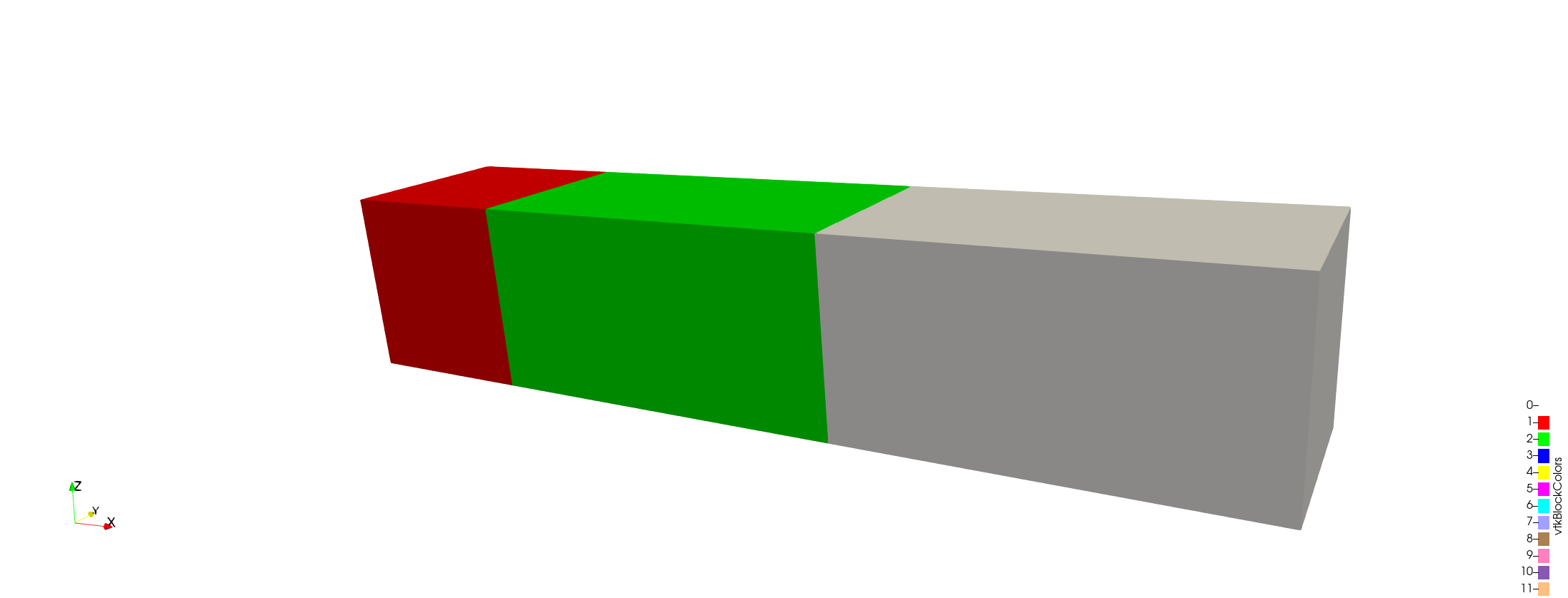
Figure 1: Beam model with the domain divided into three subdomains. The red, green, and gray colors represent three subdomains.
Mesh refinement using Indicator and Marker
MASTODON is capable of automatic mesh refinement using the MOOSE's Adaptivity System. The Adaptivity System can use an Indicator to provide measurement of "errors" for the elements (difference between the current and required refinements) about the required mesh refinement. These "errors" are passed on to a Marker to decide which elements need refinement. Alternatively, the Marker can calculate the "errors" by itself to inform the mesh refinement without relying on the Indicator. Both of these cases will be demonstrated. Specifically, the MinimumElementSizeMarker for mesh refinement is demonstrated. The MinimumElementSizeMarker is capable of refining elements based on either an indicator or an element_size value. These capabilities are first individually demonstrated below, and are then combined using the ComboMarker.
Mesh refinement using the MinimumElementSizeMarker with the indicator option
In the cantilever beam model, the goal is to refine the subdomain in green with the "errors" computed by the ShearWaveIndicator. The initial mesh is such that it has 10 partitions along the length (x-direction) and 2 partitions along the breadth and height (y- and z-directions). The shear-wave velocity of the beam model is set to 250 m/s as shown below.
  [shear_wave_speed]
    type = GenericConstantMaterial
    prop_names = shear_wave_speed
    prop_values =  250.0
  []
[]
The ShearWaveIndicator is defined in the Adaptivity block shown below with a cutoff frequency of 1000 Hz. With a shear_wave velocity of 250 m/s, this implies the minimum element size will be 0.25 m in the green subdomain computed using the formula (shear_wave velocity / cutoff frequency).
  [Indicators]
    [shear_wave]
      type = ShearWaveIndicator
      cutoff_frequency = 1000
    []
[]The Markers block has the MinimumElementSizeMarker with the indicator option, as shown below.
    [marker2]
      type = MinimumElementSizeMarker
      indicator = shear_wave
      block = 2
[] After the mesh refinement, as presented in the figure below, we see that the green subdomain has an element size less than or equal to 0.25 m, as specified by the ShearWaveIndicator. The initial element size in the green subdomain before refinement is 0.5 m.
 with the `indicator` option.](../media/examples/ex11b/ex11b_indicatormarker.png)
Figure 2: Beam model with the green subdomain's mesh refined using the MinimumElementSizeMarker with the indicator option.
Mesh refinement using the MinimumElementSizeMarker with the element_size option
Alternatively, instead of relying on an indicator, the MinimumElementSizeMarker can directly take an element_size value for the mesh refinement. This capability is demonstrated here. The goal is to refine the red subdomain in the beam such that the minimum element size is less than or equal to 0.15 m. This can be accomplished using the element_size option as shown in the code block below.
    [marker1]
      type = MinimumElementSizeMarker
      element_size = 0.15
      block = 1
[]The end result, as presented in the figure below, is the red subdomain having an element size less than 0.15 m. Additionally, it is worth noticing that the green subdomain is also refined near the interface with the red subdomain. However, we did not intend to refine the green subdomain here. This behavior is due to the nature of -adaptivity which MOOSE employs. For more information, please refer to the Adaptivity System.
 with the `element_size` option.](../media/examples/ex11b/ex11b_valuemarker.png)
Figure 3: Beam model with the red subdomain's mesh refined using the MinimumElementSizeMarker with the element_size option.
Mesh refinement using the ComboMarker
It is also possible to combine two different Markers into a single Marker with the ComboMarker option. The goal now is to combine the MinimumElementSizeMarker with the indicator option and MinimumElementSizeMarker with the element_size option. The below code block accomplishes this.
  [Markers]
    [marker1]
      type = MinimumElementSizeMarker
      element_size = 0.15
      block = 1
    []
    [marker2]
      type = MinimumElementSizeMarker
      indicator = shear_wave
      block = 2
    []
    [combo]
      type = ComboMarker
      markers = 'marker1 marker2'
      block = '1 2'
    []
  []
[]
The figure below presents the mesh of the beam after refinement using the ComboMarker. Notice that even though the goal is to refine the red subdomain to have an element size less than 0.15 m and the green subdomain to have an element size less than 0.25 m, both these subdomains have an element size less than 0.15 m. This behavior is due to how the ComboMarker operates. Given several Markers, the ComboMarker refines all the associated subdomains based on the greatest refinement required across all the given Markers and their subdomains. That is, the mesh for each of the associated subdomains is refined to the maximum level of refinement allowed by the limiting marker.
.](../media/examples/ex11b/ex11b_combomarker.png)
Figure 4: Beam model with the red and green subdomains' mesh refined using the ComboMarker.
Demonstration of SidesetMoment and AverageValue postprocessors
Often during analyses of structures, we are required to compute auxiliary quantities such as stresses and moments which are dependent on the primary variables, the displacements. These auxiliary quantities are computed using postprocessors. In this example, two types of postprocessors (namely, SidesetMoment and AverageValue) are demonstrated.
SidesetMoment postprocessor
SidesetMoment is a generic postprocessor used for computing moments about a required axis acting at a reference point on a sideset. Therefore, this postprocessor takes the reference point coordinates and either stress or pressure as some of the inputs. Stress is used in this example. In addition, it requires the stress and moment directions. These directions should be defined such that their cross product should be the direction about which the moment acts. For example, in the code block below, it is desired to compute the moment at the left end (i.e., the fixed end) of the beam about the z-axis. Now, the stress direction is defined as (1,0,0) and the moment direction is defined as (0,0,1) to give the moment about the z-axis. For more information, please refer to SidesetMoment.
  [moment_z]
    type = SidesetMoment
    stress_direction = '1 0 0'
    stress_tensor = stress
    boundary = 'left'
    reference_point = '0.0 0.0 0.5'
    moment_direction = '0 0 1'
[]The computed moment from stresses using the SidesetMoment postprocessor is 5.18 KN. Where as, the applied moment at this sideset is 5 KN. It is seen that the computed and applied moments are quite close, with an error of about 3.6 %. This error can be further reduced by refinement of the mesh. For example, with a more refined mesh, we obtained a computed moment of 5.03 KN, which has an error of about 0.6 %. These results highlight the sensitivity of stresses and the resulting moment computed using stresses to the mesh refinement.
SideAverageValue and ElementAverageValue postprocessors
Both SideAverageValue and ElementAverageValue postprocessors compute averaged values of quantities (such as stresses or displacements) across a sideset and subdomain, respectively. The below code block uses these two postprocessors to compute averaged stress in the x-direction across a sideset and a subdomain.
  [avg_stress_xx_side]
    type = SideAverageValue
    variable = stress_xx
    boundary = left
  []
  [avg_stress_xx_block]
    type = ElementAverageValue
    variable = stress_xx
    block = 1
  []
[]
The computed average stress across the left end sideset and the red subdomain of the beam are both close to zero. Theoretically, these close to zero values are due to the symmetry of the stress distribution along the depth of the beam.
A complete list of the postprocessor results are presented in the table below.
Table 1: Postprocessor values computed using two levels of mesh refinement.
| Value | Level 1 refinement | Level 2 refinement |
|---|---|---|
| SidesetMoment | 5.18 KN (Exact = 5 KN) | 5.03 KN (Exact = 5 KN) |
SideAverageValue for stress_xx | 0.0063 Pa (Exact = 0 Pa) | 1E-12 Pa (Exact = 0 Pa) |
ElementAverageValue for stress_xx | 0.01 Pa (Exact = 0 Pa) | 1E-12 Pa (Exact = 0 Pa) |