Problem with Analytical Solution
Introduction
The best method for verifying a simulation is comparison with a known mathematical solution. For the heat equation, as defined in FEM Convergence, one such solution shall be considered to verify a model. The verification process shall be broken into four parts:
Define a problem, with a known exact solution.
Simulate the problem.
Compute the error between the known solution and the simulation.
Perform convergence study.
Problem Statement
Incropera et al. (1996) presents a one-dimensional solution for the heat equation as:
(1)where is the temperature, is the initial temperature, is time, is position, is the heat source, is thermal conductivity, and is the thermal diffusivity.
Thermal diffusivity is defined as the ratio of thermal conductivity () to the product of density () and specific heat capacity (). The system is subjected to Neumann boundary conditions at the left boundary () and the natural boundary condition (zero flux) on the opposite boundary.
Simulation
The heat transfer module of MOOSE is capable of performing a simulation of the above problem without modification. The values presented in Table 1 were selected for the simulation and a duration of 1 second shall be utilized.
Table 1: Numerical values used to the solution values of Eq. (1).
| Variable | Value | Units |
|---|---|---|
| 300 | ||
| 7E5 | ||
| 80.2 | ||
| 7800 | ||
| 450 | ||
| 7E5 | ||
| 0 |
Simulation Setup
The following instructions assumes that there is a working version of MOOSE installed on the system, for information on getting it setup please refer to the install instructions.
The simulation to be performed relies on the heat transfer module, thus it is necessary to compile that specific module. It is assumed that MOOSE was cloned into a directory named "projects" within the home directory. With this assumption, the following commands will compile and test the heat transfer module executable.
cd ~/projects/moose/modules/heat_transfer
make -j8
./run_tests -j8
The number used after the "-j" should be the number of processes available on your system. If tests execute without failure, then the following sections should be followed to setup the simulation.
Simulation Input
MOOSE operates using input files, as such, an input file is detailed below that is capable of simulating this problem and its use demonstrated. This section will describe the various sections of the input file that should be created for the current problem. The location of this input file is arbitrary, but it is assumed that the content below will be in a file named ~/projects/problems/verification/1d_analytical.i. This file can be created and edited using any text editor program.
Within this file, the domain of the problem is defined using the Mesh System using the [Mesh] block of the input file, as follows, which creates a one-dimensional mesh in the -direction from 0 to 0.03 using 200 elements.
[Mesh<<<{"href": "../../../syntax/Mesh/index.html"}>>>]
  [gen]
    type = GeneratedMeshGenerator<<<{"description": "Create a line, square, or cube mesh with uniformly spaced or biased elements.", "href": "../../../source/meshgenerators/GeneratedMeshGenerator.html"}>>>
    dim<<<{"description": "The dimension of the mesh to be generated"}>>> = 1
    xmax<<<{"description": "Upper X Coordinate of the generated mesh"}>>> = 0.03
    nx<<<{"description": "Number of elements in the X direction"}>>> = 200
  []
[]
There is a single unknown, temperature (), to compute. This unknown is declared using the Variables System in the [Variables] block and used the default configuration of a first-order Lagrange finite element variable. Note, within this block the name of the variable is arbitrary; "T" was selected here to match the equation.
[Variables<<<{"href": "../../../syntax/Variables/index.html"}>>>]
  [T]
  []
[]
The initial condition for temperature at the beginning of the simulation is set using the Initial Condition System in the [ICs] block. At , an constant initial value of is applied uniformly across the problem.
[ICs<<<{"href": "../../../syntax/ICs/index.html"}>>>]
  [T_O]
    type = ConstantIC<<<{"description": "Sets a constant field value.", "href": "../../../source/ics/ConstantIC.html"}>>>
    variable<<<{"description": "The variable this initial condition is supposed to provide values for."}>>> = T
    value<<<{"description": "The value to be set in IC"}>>> = 300
  []
[]
The "volumetric" portions of the weak form are defined using the Kernel System in the [Kernels] block, for this example this can be done with the use of two Kernel objects as follows.
[Kernels<<<{"href": "../../../syntax/Kernels/index.html"}>>>]
  [T_time]
    type = HeatConductionTimeDerivative<<<{"description": "Time derivative term $\\rho c_p \\frac{\\partial T}{\\partial t}$ of the thermal energy conservation equation.", "href": "../../../source/kernels/HeatConductionTimeDerivative.html"}>>>
    variable<<<{"description": "The name of the variable that this residual object operates on"}>>> = T
    density_name<<<{"description": "Property name of the density material property"}>>> = 7800
    specific_heat<<<{"description": "Name of the volumetric isobaric specific heat material property"}>>> = 450
  []
  [T_cond]
    type = HeatConduction<<<{"description": "Diffusive heat conduction term $-\\nabla\\cdot(k\\nabla T)$ of the thermal energy conservation equation", "href": "../../../source/kernels/HeatConduction.html"}>>>
    variable<<<{"description": "The name of the variable that this residual object operates on"}>>> = T
    diffusion_coefficient = 80.2
  []
[]
The sub-block "T_time" defines the time derivative and "T_cond" defines the conduction portion of the equation, please refer to Heat Conduction for details regarding the weak form of the heat equation. Both blocks include the "variable" parameter, which is set equal to "T". The remaining parameters define the values for , , and as the constant values defined in Table 1.
The boundary portions of the weak form are defined using the Boundary Condition System in the [BCs] block. At a Neumann condition is applied with a value of 7E5. The generated mesh, by default, labels the boundary at as "left".
[BCs<<<{"href": "../../../syntax/BCs/index.html"}>>>]
  [left]
    type = NeumannBC<<<{"description": "Imposes the integrated boundary condition $\\frac{\\partial u}{\\partial n}=h$, where $h$ is a constant, controllable value.", "href": "../../../source/bcs/NeumannBC.html"}>>>
    variable<<<{"description": "The name of the variable that this residual object operates on"}>>> = T
    boundary<<<{"description": "The list of boundary IDs from the mesh where this object applies"}>>> = left
    value<<<{"description": "For a Laplacian problem, the value of the gradient dotted with the normals on the boundary."}>>> = 7e5
  []
[]
The natural boundary condition does not require definition, as the name suggests, this condition is applied naturally based on the weak form derivation.
The problem is solved using Newton's method with a second-order backward difference formula (BDF2) with a timestep of 0.01 seconds up to a simulation time of one second. These settings are applied within the [Executioner] block using the Executioner System.
[Executioner<<<{"href": "../../../syntax/Executioner/index.html"}>>>]
  type = Transient
  scheme = bdf2
  solve_type = NEWTON
  dt = 0.01
  end_time = 1
[]
Finally, the output method is defined. In this case the ExodusII and CSV format are enabled within the [Outputs] block using the Outputs System.
[Outputs<<<{"href": "../../../syntax/Outputs/index.html"}>>>]
  exodus<<<{"description": "Output the results using the default settings for Exodus output."}>>> = true
  csv<<<{"description": "Output the scalar variable and postprocessors to a *.csv file using the default CSV output."}>>> = true
[]
Simulation Execution
Executing the simulation is straightforward, simply execute the heat transfer module executable with the input file included using the "-i" option as follows.
cd ~/projects/moose/tutorials/tutorial03_verification/step03_analytical
~/projects/moose/modules/heat_transfer/heat_conduction-opt -i 1d_analytical.i
When complete an output file will be produced with the name "1d_analytical_out.e", this file can be viewed using Paraview or Peacock.
Compute Error
To be able to compute the error with respect to the known solution, Eq. (1) must be added to the input file. This is accomplished via a ParsedFunction object that is added in the [Functions] block.
[Functions<<<{"href": "../../../syntax/Functions/index.html"}>>>]
  [T_exact]
    type = ParsedFunction<<<{"description": "Function created by parsing a string", "href": "../../../source/functions/MooseParsedFunction.html"}>>>
    symbol_names<<<{"description": "Symbols (excluding t,x,y,z) that are bound to the values provided by the corresponding items in the symbol_values vector."}>>> = 'k    rho  cp  T0  qs'
    symbol_values<<<{"description": "Constant numeric values, postprocessor names, function names, and scalar variables corresponding to the symbols in symbol_names."}>>> = '80.2 7800 450 300 7e5'
    expression<<<{"description": "The user defined function."}>>> = 'T0 + qs/k*(2*sqrt(k/(rho*cp)*t/pi)*exp(-x^2/(4*k/(rho*cp)*(t+1e-50))) - x*(1-erf(x/(2*sqrt(k/(rho*cp)*(t+1e-50))))))'
  []
[]
The "symbol_names" and "symbol_values" items have a one-to-one relationship, e.g., . If defined in this manner then the names in "symbol_names" can be used in the definition of the equation in the "expression" parameter.
The error is a single value for each time step. Since the exact solution is known the -norm can be computed using the ElementL2Error object within the [Postprocessors] block, which computes the error of the given variable (e.g., "T") and the known solution defined in the "T_exact" function.
[Postprocessors<<<{"href": "../../../syntax/Postprocessors/index.html"}>>>]
  [error]
    type = ElementL2Error<<<{"description": "Computes L2 error between a field variable and an analytical function", "href": "../../../source/postprocessors/ElementL2Error.html"}>>>
    variable<<<{"description": "The name of the variable that this object operates on"}>>> = T
    function<<<{"description": "The analytic solution to compare against"}>>> = T_exact
  []
  [h]
    type = AverageElementSize<<<{"description": "Computes the average element size.", "href": "../../../source/postprocessors/AverageElementSize.html"}>>>
  []
[]
In addition to the computed error, the average element size is also output. As detailed previously, this quantity is necessary to perform the convergence study.
Another useful item to add to the input, especially for a one-dimensional problem, are line samples along the length of the simulation for the computed and exact solution via the [VectorPostprocessors] block.
[VectorPostprocessors<<<{"href": "../../../syntax/VectorPostprocessors/index.html"}>>>]
  [T_exact]
    type = LineFunctionSampler<<<{"description": "Sample one or more functions along a line.", "href": "../../../source/vectorpostprocessors/LineFunctionSampler.html"}>>>
    functions<<<{"description": "The Functions to sample along the line"}>>> = T_exact
    start_point<<<{"description": "The beginning of the line"}>>> = '0 0 0'
    end_point<<<{"description": "The ending of the line"}>>> = '0.03 0 0'
    num_points<<<{"description": "The number of points to sample along the line"}>>> = 200
    sort_by<<<{"description": "What to sort the samples by. Options include 'x', 'y', 'z', 'id', and the name of any of the sampled quantities (which each create a vector of the same name)."}>>> = x
    execute_on<<<{"description": "The list of flag(s) indicating when this object should be executed. For a description of each flag, see https://mooseframework.inl.gov/source/interfaces/SetupInterface.html."}>>> = 'INITIAL TIMESTEP_END'
  []
  [T_simulation]
    type = LineValueSampler<<<{"description": "Samples variable(s) along a specified line", "href": "../../../source/vectorpostprocessors/LineValueSampler.html"}>>>
    variable<<<{"description": "The names of the variables that this VectorPostprocessor operates on"}>>> = T
    start_point<<<{"description": "The beginning of the line"}>>> = '0 0 0'
    end_point<<<{"description": "The ending of the line"}>>> = '0.03 0 0'
    num_points<<<{"description": "The number of points to sample along the line"}>>> = 200
    sort_by<<<{"description": "What to sort the samples by. Options include 'x', 'y', 'z', 'id', and the name of any of the sampled quantities (which each create a vector of the same name)."}>>> = x
    execute_on<<<{"description": "The list of flag(s) indicating when this object should be executed. For a description of each flag, see https://mooseframework.inl.gov/source/interfaces/SetupInterface.html."}>>> = 'INITIAL TIMESTEP_END'
  []
[]
In this block the both the exact solution function ("T_exact") and the finite element solution ("T") are sampled along the length of the simulation. The -norm as well as these line sampled values are both output as CSV files for further analysis.
Figure 1 shows the complete results, including the simulated solution, the exact solution, and the absolute error as a function of simulation time.
Figure 1: Comparison of simulation results, the exact solution, and the computed absolute error for the one-dimensional heat equation.
Convergence Studies
As shown in Figure 1 the results obtained from the simulation seem to agree well with the known solution. The results provide evidence that the finite element calculations are being performed correctly. As is, the error shown could be due to a problem with the finite element implementation. However, if the error is reduced at the expected rate with decreasing mesh size and timestep size then it is reasonable that the finite element formulation and temporal numerical integration are implemented correctly.
MOOSE includes a python package—the mms package—for performing convergence studies, which will be used here. For details regarding the package, please refer to the Method of Manufactured Solutions (MMS) documentation.
Spatial Convergence
To perform a spatial convergence the input file created needs to be executed with decreasing element size, which in MOOSE can be done by adding the Mesh/uniform_refine=x option to the command line with "x" being an integer representing the number of refinements to perform.
The mms package includes a function (run_spatial) for performing and automatically modifying the supplied input file to perform increasing levels of uniform refinement. After each run the results are collected into a pandas.DataFrame object, which can be used in the ConvergencePlot object to create a plot.
For example, for Listing 1 results of the spatial convergence study are shown as a plot in Figure 2. In this case, the input file created above (1d_analytical.i) is executed with six levels of uniform refinement (0–5). Notice that an extra argument Mesh/nx=10 is supplied to reduce the number of elements to 10 for the initial mesh. The console flag suppress the screen output from the simulations.
Listing 1: Example use of the mms package to run and plot spatial convergence.
import mms

df = mms.run_spatial("1d_analytical.i", 6, "Mesh/gen/nx=10", console=False)
fig = mms.ConvergencePlot(xlabel="Element Size ($h$)", ylabel="$L_2$ Error")
fig.plot(df, label="1st Order", marker="o", markersize=8)
fig.save("1d_analytical_spatial.png")
The resulting convergence data indicate that the simulation is converging to the known solution at the correct rate for first-order elements, thus verifying that the finite element solution is computing the results as expected.
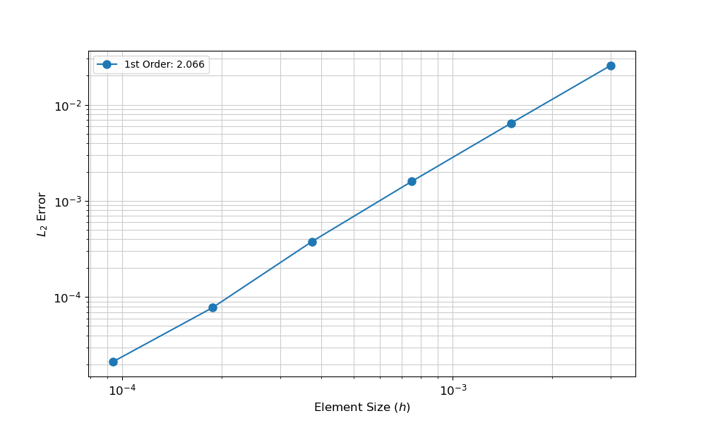
Figure 2: Results of the spatial convergence study comparing the finite element simulation with the known one-dimensional analytical solution.
Temporal Convergence
The temporal convergence study is nearly identical to the spatial, as shown in Listing 2. For a temporal study, the run_temporal is used and the initial time step is set using dt; the number of elements is not altered. The resulting converge graph is shown in Figure 3.
Listing 2: Example use of the mms package to run and plot temporal convergence.
import mms

df = mms.run_temporal("1d_analytical.i", 6, dt=0.5, console=False)
fig = mms.ConvergencePlot(xlabel="$\\Delta t$", ylabel="$L_2$ Error")
fig.plot(df, label="2nd Order (Backward Difference)", marker="o", markersize=8)
fig.save("1d_analytical_temporal.png")
The resulting convergence data indicate that the simulation is converging to the known solution at the correct rate for second-order time integration, thus verifying that the numerical integration scheme is operating as expected.
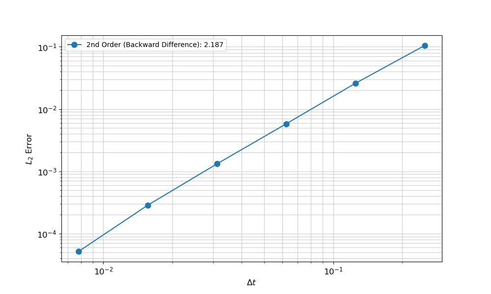
Figure 3: Results of the spatial convergence study comparing the finite element simulation with the known one-dimensional analytical solution.
Closing Remarks
The analysis performed here provides three levels of verification: (1) the finite element solution matches the known solution with minimal error, (2) the spatial error converges at the expected rate for first-order finite elements, and (3) the temporal error converges at the expected rate for second-order numerical integration. These results verify that the simulation is correctly solving the 1D heat equation.
References
- Frank P Incropera, David P DeWitt, Theodore L Bergman, Adrienne S Lavine, and others.
Fundamentals of heat and mass transfer.
Volume 6.
Wiley New York, 1996.[Export]