Method of Manufactured Solution
Introduction
In practice an exact solution to the problem being solved is rarely known, since there would be no reason to perform a simulation if the answer is known. If the solution is not known then the error cannot be computed. However, it is possible to "manufacture" a solution using a method known as the Method of Manufactured Solutions (MMS). In this step of the tutorial the two-dimensional heat equation will be used to simulate a physical system. Then using this simulation as a starting point a spatial and temporal convergence study will be performed using the MMS.
Problem Statement
For this example, the two-dimensional heat equation shall be used to simulate a cross section of snow subjected to radiative cooling at the surface and internal heating due to solar absorption.
The domain of the problem is defined as and . Referring to the heat equation defined in Step 1, a heat source () is applied as defined in Eq. (1). This source is a crude approximation of internal heating due to solar absorption. The source raised from zero to a maximum of 650 back to zero during a 9 hours (32400 sec.) period following a sine function. The duration is an approximation of the daylight hours in Idaho Falls, Idaho in December. Also, the left side of the domain is shaded and the right is subjected to the maximum source, again defined using a sine function.
(1)where is the extinction coefficient.
The system is subjected to Neumann boundary conditions at the top surface boundary (), which approximates the radiative cooling of the snow surface. The left and right sides of the domain are subjected to the natural boundary condition, which for this problem approximates an "insulated" boundary condition. Finally, a constant temperature is imposed on the bottom boundary.
Simulation
The heat transfer module of MOOSE is capable of performing the desired simulation. The values in Table 1 provide the numeric values to be used for the simulation, which will solve for nine hours of simulation time.
Table 1: Numerical values used for two-dimensional simulation of snow.
| Variable | Value | Units |
|---|---|---|
| 263.15 | ||
| 0.01 | ||
| 150 | ||
| 2000 | ||
| 40 | ||
| -5 | ||
| 263.15 |
As in the previous step, a complete input file will be explained block by block. It shall be assumed that the input file is named ~/projects/problems/verification/2d_main.i. This file can be created and edited using any text editor program.
The problem requires a two-dimensional rectangular domain, which can be defined using the Mesh System as defined in the [Mesh] block of the input. The number of elements ("nx" and "ny") are defined to result in square elements.
[Mesh<<<{"href": "../../../syntax/Mesh/index.html"}>>>]
  [gen]
    type = GeneratedMeshGenerator<<<{"description": "Create a line, square, or cube mesh with uniformly spaced or biased elements.", "href": "../../../source/meshgenerators/GeneratedMeshGenerator.html"}>>>
    dim<<<{"description": "The dimension of the mesh to be generated"}>>> = 2
    ymax<<<{"description": "Upper Y Coordinate of the generated mesh"}>>> = 0
    ymin<<<{"description": "Lower Y Coordinate of the generated mesh"}>>> = -0.2
    nx<<<{"description": "Number of elements in the X direction"}>>> = 20
    ny<<<{"description": "Number of elements in the Y direction"}>>> = 4
  []
[]
There is a single unknown, temperature (), to compute. This unknown is declared using the Variables System in the [Variables] block and used the default configuration of a first-order Lagrange finite element variable.
[Variables<<<{"href": "../../../syntax/Variables/index.html"}>>>]
  [T]
  []
[]
The initial condition () is applied using the Initial Condition System in the [ICs] block. In this case a constant value throughout the domain is provided.
[ICs<<<{"href": "../../../syntax/ICs/index.html"}>>>]
  [T_O]
    type = ConstantIC<<<{"description": "Sets a constant field value.", "href": "../../../source/ics/ConstantIC.html"}>>>
    variable<<<{"description": "The variable this initial condition is supposed to provide values for."}>>> = T
    value<<<{"description": "The value to be set in IC"}>>> = 263.15
  []
[]
The volumetric heat source, , is defined using the Function System using the [Functions] block. The function, as defined in Eq. (1) can be defined directly in the input file using the parsed function capability. The "symbol_names" and "symbol_values" parameters are used to define named constants within the equation. The variables "x", "y", "z", and "t" are always available and represent the corresponding spatial location and time.
[Functions<<<{"href": "../../../syntax/Functions/index.html"}>>>]
  [source]
    type = ParsedFunction<<<{"description": "Function created by parsing a string", "href": "../../../source/functions/MooseParsedFunction.html"}>>>
    symbol_names<<<{"description": "Symbols (excluding t,x,y,z) that are bound to the values provided by the corresponding items in the symbol_values vector."}>>> = 'hours shortwave kappa'
    symbol_values<<<{"description": "Constant numeric values, postprocessor names, function names, and scalar variables corresponding to the symbols in symbol_names."}>>> = '9     650      40'
    expression<<<{"description": "The user defined function."}>>> = 'shortwave*sin(0.5*x*pi)*exp(kappa*y)*sin(1/(hours*3600)*pi*t)'
  []
[]
The "volumetric" portion of the weak form are defined using the Kernel System in the [Kernels] block, for this example this can be done with the use of three Kernel objects as follows.
[Kernels<<<{"href": "../../../syntax/Kernels/index.html"}>>>]
  [T_time]
    type = HeatConductionTimeDerivative<<<{"description": "Time derivative term $\\rho c_p \\frac{\\partial T}{\\partial t}$ of the thermal energy conservation equation.", "href": "../../../source/kernels/HeatConductionTimeDerivative.html"}>>>
    variable<<<{"description": "The name of the variable that this residual object operates on"}>>> = T
    density_name<<<{"description": "Property name of the density material property"}>>> = 150
    specific_heat<<<{"description": "Name of the volumetric isobaric specific heat material property"}>>> = 2000
  []
  [T_cond]
    type = HeatConduction<<<{"description": "Diffusive heat conduction term $-\\nabla\\cdot(k\\nabla T)$ of the thermal energy conservation equation", "href": "../../../source/kernels/HeatConduction.html"}>>>
    variable<<<{"description": "The name of the variable that this residual object operates on"}>>> = T
    diffusion_coefficient = 0.01
  []
  [T_source]
    type = HeatSource<<<{"description": "Demonstrates the multiple ways that scalar values can be introduced into kernels, e.g. (controllable) constants, functions, and postprocessors. Implements the weak form $(\\psi_i, -f)$.", "href": "../../../source/kernels/HeatSource.html"}>>>
    variable<<<{"description": "The name of the variable that this residual object operates on"}>>> = T
    function<<<{"description": "Function describing the volumetric heat source"}>>> = source
  []
[]
The sub-block "T_time" defines the time derivative, "T_cond" defines the conduction portion of the equation, and "T_source" defines the heat source term, please refer to Heat Conduction for details regarding the weak form of the heat equation. All blocks include the "variable" parameter, which is set equal to "T". The remaining parameters define the values for , , and as the constant values defined in Table 1.
The boundary portions of the weak form are defined using the Boundary Condition System in the [BCs] block. At top of the domain () a Neumann condition is applied with a constant outward flux. On the bottom of the domain () a constant temperature is defined.
[BCs<<<{"href": "../../../syntax/BCs/index.html"}>>>]
  [top]
    type = NeumannBC<<<{"description": "Imposes the integrated boundary condition $\\frac{\\partial u}{\\partial n}=h$, where $h$ is a constant, controllable value.", "href": "../../../source/bcs/NeumannBC.html"}>>>
    boundary<<<{"description": "The list of boundary IDs from the mesh where this object applies"}>>> = top
    variable<<<{"description": "The name of the variable that this residual object operates on"}>>> = T
    value<<<{"description": "For a Laplacian problem, the value of the gradient dotted with the normals on the boundary."}>>> = -5
  []
  [bottom]
    type = DirichletBC<<<{"description": "Imposes the essential boundary condition $u=g$, where $g$ is a constant, controllable value.", "href": "../../../source/bcs/DirichletBC.html"}>>>
    boundary<<<{"description": "The list of boundary IDs from the mesh where this object applies"}>>> = bottom
    variable<<<{"description": "The name of the variable that this residual object operates on"}>>> = T
    value<<<{"description": "Value of the BC"}>>> = 263.15
  []
[]
The remain boundaries are "insulated", which is known as the natural boundary condition. This does not require definition, as the name suggests, this condition is applied naturally based on the weak form derivation.
The problem is solved using Newton's method with a first-order backward Euler method with a timestep of 600 seconds (10 min.) up to a simulation time of nine hours. These settings are applied within the [Executioner] block using the Executioner System.
[Executioner<<<{"href": "../../../syntax/Executioner/index.html"}>>>]
  type = Transient
  solve_type = 'NEWTON'
  dt = 600 # 10 min
  end_time = 32400 # 9 hour
[]
Finally, the output method is defined. In this case the ExodusII format is enabled within the [Outputs] block using the Outputs System.
[Outputs<<<{"href": "../../../syntax/Outputs/index.html"}>>>]
  exodus<<<{"description": "Output the results using the default settings for Exodus output."}>>> = true
[]
Simulation Execution
Executing the simulation is straightforward, simply execute the heat transfer module executable with the input file included using the "-i" option as follows.
cd ~/projects/problems/verification
../../moose/modules/heat_transfer/heat_conduction-opt -i 2d_main.i
When complete an output file will be produced with the name "2d_main_out.e", this file can be viewed using Paraview or Peacock. Figure 1 show the change in temperature across the domain with time. A key feature is that the surface remains cool as the heat source warms the snow internally, creating large temperature gradient at the surface.
Figure 1: Simulation results for application of the heat equation for simulating snow in two-dimensions.
MMS Overview
The MMS is a method of manufacturing a known solution for a partial differential equation (PDE), in this case the transient heat equation. The method is explained in detail in the context of the mms python package included with MOOSE: Method of Manufactured Solutions (MMS). A brief overview shall be provided here, but the reader is referred to the package documentation for a more detailed description.
The method can be summarized into three basic steps:
Define an assumed solution for the PDE of interest, for example .
schooltip:Select a solution that cannot be represented exactly.The form of the solution is arbitrary, but certain characteristics are desirable. Mainly, a solution should be selected that cannot be exactly represented by the Finite Element Method (FEM) shape function or the numerical integration scheme, for spatial and temporal convergence studies, respectively. Without these characteristic the assumed solution could possibly be solved exactly, thus there will not be error and the rate of convergence to the solution cannot be examined.
Apply the assumed solution to the PDE to compute a residual function. For example, consider the following simple PDE.
Substitute the assumed solution of into this equation to compute the residual.
Apply the negative of the computed function and perform the desired convergence study. For example, the example PDE above becomes:
This PDE has a known solution, , that can be used to compute the error and perform a convergence study.
While it is possible to perform these steps with hand calculations, this can become difficult and error prone for more complex equations. For this reason the mms python package included with MOOSE was created. This package will be used to apply these steps to the two-dimensional heat equation example defined above.
Spatial Convergence
The first step of using the MMS involves assuming a solution to the desired PDE, which in this case is the transient heat equation with a source term. Eq. (2) shall be the assumed solution for the spatial study.
(2)The assumed solution has two characteristics: it cannot be exactly represented by the first-order FEM shape functions and the first-order time integration can exactly capture the time portion of the equation and not result in temporal error accumulation.
The mms package, as shown in Listing 1, is used to compute the necessary forcing function. The package can directly output the input file format for the computed forcing function and the assumed solution, making adding it to the input file trivial.
Listing 1: Compute the forcing function using MMS.
import mms

fs, ss = mms.evaluate(
    (
        "rho * cp * diff(u,t) - div(k*grad(u)) - "
        "shortwave*sin(0.5*x*pi)*exp(kappa*y)*sin(1/(hours*3600)*pi*t)"
    ),
    "t*sin(pi*x)*sin(5*pi*y)",
    scalars=["rho", "cp", "k", "kappa", "shortwave", "hours"],
)
mms.print_hit(fs, "mms_force")
mms.print_hit(ss, "mms_exact")
Executing this script, assuming a name of spatial_function.py results in the following output.
$ python spatial_function.py
[mms_force]
  type = ParsedFunction
  expression = 'cp*rho*sin(x*pi)*sin(5*y*pi) + 26*pi^2*k*t*sin(x*pi)*sin(5*y*pi) - shortwave*exp(y*kappa)*sin((1/2)*x*pi)*sin((1/3600)*pi*t/hours)'
  symbol_names = 'hours rho shortwave k cp kappa'
  symbol_values = '1.0 1.0 1.0 1.0 1.0 1.0'
[]
[mms_exact]
  type = ParsedFunction
  expression = 't*sin(x*pi)*sin(5*y*pi)'
[]
Obviously, when adding to the input file the "symbol_values" must be updated to the correct values for the desired simulation.
MOOSE allows for multiple input files to be supplied to an executable, when this is done the inputs are combined into a single file that comprises the union of the two files. As such, the additional blocks required to perform the spatial convergence study and be created in an independent file. It shall be assumed this file is named ~/projects/problems/verification/2d_mms_spatial.i.
The forcing function and exact solution are added using a parsed function, similar to the existing functions within the simulation.
[Functions<<<{"href": "../../../syntax/Functions/index.html"}>>>]
  [mms_force]
    type = ParsedFunction<<<{"description": "Function created by parsing a string", "href": "../../../source/functions/MooseParsedFunction.html"}>>>
    expression<<<{"description": "The user defined function."}>>> = 'cp*rho*sin(x*pi)*sin(5*y*pi) + 26*pi^2*k*t*sin(x*pi)*sin(5*y*pi) - shortwave*exp(y*kappa)*sin((1/2)*x*pi)*sin((1/3600)*pi*t/hours)'
    symbol_names<<<{"description": "Symbols (excluding t,x,y,z) that are bound to the values provided by the corresponding items in the symbol_values vector."}>>> = 'rho cp   k     kappa shortwave hours'
    symbol_values<<<{"description": "Constant numeric values, postprocessor names, function names, and scalar variables corresponding to the symbols in symbol_names."}>>> = '150 2000 0.01  40    650       9'
  []
  [mms_exact]
    type = ParsedFunction<<<{"description": "Function created by parsing a string", "href": "../../../source/functions/MooseParsedFunction.html"}>>>
    expression<<<{"description": "The user defined function."}>>> = 't*sin(pi*x)*sin(5*pi*y)'
  []
[]
The forcing function is applied to the simulation by adding another heat source Kernel object.
[Kernels<<<{"href": "../../../syntax/Kernels/index.html"}>>>]
  [mms]
    type = HeatSource<<<{"description": "Demonstrates the multiple ways that scalar values can be introduced into kernels, e.g. (controllable) constants, functions, and postprocessors. Implements the weak form $(\\psi_i, -f)$.", "href": "../../../source/kernels/HeatSource.html"}>>>
    variable<<<{"description": "The name of the variable that this residual object operates on"}>>> = T
    function<<<{"description": "Function describing the volumetric heat source"}>>> = mms_force
  []
[]
To perform the study the error and element size are required, these are added as Postprocessors as done in the previous example in Step 03.
[Postprocessors<<<{"href": "../../../syntax/Postprocessors/index.html"}>>>]
  [error]
    type = ElementL2Error<<<{"description": "Computes L2 error between a field variable and an analytical function", "href": "../../../source/postprocessors/ElementL2Error.html"}>>>
    variable<<<{"description": "The name of the variable that this object operates on"}>>> = T
    function<<<{"description": "The analytic solution to compare against"}>>> = mms_exact
  []
  [h]
    type = AverageElementSize<<<{"description": "Computes the average element size.", "href": "../../../source/postprocessors/AverageElementSize.html"}>>>
  []
[]
CSV output also needs to be added,
[Outputs<<<{"href": "../../../syntax/Outputs/index.html"}>>>]
  csv<<<{"description": "Output the scalar variable and postprocessors to a *.csv file using the default CSV output."}>>> = true
[]
At this point, it is tempting to perform the study and the reader is encouraged to do so; however, the results will be disappointing. The reason is that the initial and boundary conditions for the simulation do not satisfy the assumed solution. In most cases, unless the study is testing the boundary condition object specifically, the easiest approach is to use the assumed solution to set both the initial condition and boundary conditions. This can be done by adding function based initial and boundary condition objects, and setting the "active" line which will disable all sub-blocks not listed.
[BCs<<<{"href": "../../../syntax/BCs/index.html"}>>>]
  active<<<{"description": "If specified only the blocks named will be visited and made active"}>>> = 'mms'
  [mms]
    type = FunctionDirichletBC<<<{"description": "Imposes the essential boundary condition $u=g(t,\\vec{x})$, where $g$ is a (possibly) time and space-dependent MOOSE Function.", "href": "../../../source/bcs/FunctionDirichletBC.html"}>>>
    variable<<<{"description": "The name of the variable that this residual object operates on"}>>> = T
    boundary<<<{"description": "The list of boundary IDs from the mesh where this object applies"}>>> = 'left right top bottom'
    function<<<{"description": "The forcing function."}>>> = mms_exact
  []
[]
[ICs<<<{"href": "../../../syntax/ICs/index.html"}>>>]
  active<<<{"description": "If specified only the blocks named will be visited and made active"}>>> = 'mms'
  [mms]
    type = FunctionIC<<<{"description": "An initial condition that uses a normal function of x, y, z to produce values (and optionally gradients) for a field variable.", "href": "../../../source/ics/FunctionIC.html"}>>>
    variable<<<{"description": "The variable this initial condition is supposed to provide values for."}>>> = T
    function<<<{"description": "The initial condition function."}>>> = mms_exact
  []
[]
As was the case in the previous step of this tutorial, the mms package can be used to perform the convergence study. In this case, both a first and second-order shape functions are considered.
Listing 2: Example use of the mms package to run and plot spatial convergence.
import mms

df1 = mms.run_spatial(["2d_main.i", "2d_mms_spatial.i"], 4, console=False)
df2 = mms.run_spatial(
    ["2d_main.i", "2d_mms_spatial.i"],
    4,
    "Mesh/second_order=true",
    "Variables/T/order=SECOND",
    console=False,
)

fig = mms.ConvergencePlot(xlabel="Element Size ($h$)", ylabel="$L_2$ Error")
fig.plot(df1, label="1st Order", marker="o", markersize=8)
fig.plot(df2, label="2nd Order", marker="o", markersize=8)
fig.save("2d_mms_spatial.png")
The resulting convergence data indicate that the simulation is converging to the known solution at the correct rate for first and second-order elements, thus verifying that the finite element solution is computing the results as expected.
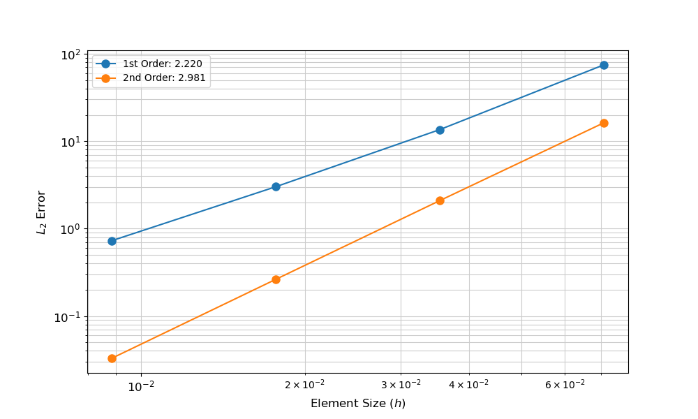
Figure 2: Results of the spatial convergence study comparing the finite element simulation with the assumed two-dimensional solution.
Temporal Convergence
The temporal convergence study is performed in the same manner as the spatial study. First, an assumed solution is selected as defined in Eq. (3). In this case, the spatial portion can be represented exactly by the shape functions and the temporal function cannot be represented by the numerical time integration scheme. A decay function is selected that has minimal changes in time and tends to an easy-to-recognize solution of xy.
Again, the mms package, as shown in Listing 3, is used to compute the necessary forcing function. The package can directly output the input file format of the computed forcing function and the assumed solution, making adding it to the input file trivial.
Listing 3: Compute the forcing function using MMS.
import mms

fs, ss = mms.evaluate(
    (
        "rho * cp * diff(u,t) - div(k*grad(u)) - "
        "shortwave*sin(0.5*x*pi)*exp(kappa*y)*sin(1/(hours*3600)*pi*t)"
    ),
    "x*y*exp(-1/32400*t)",
    scalars=["rho", "cp", "k", "kappa", "shortwave", "hours"],
)
mms.print_hit(fs, "mms_force")
mms.print_hit(ss, "mms_exact")
Executing this script, assuming a name of temporal_function.py results in the following output.
$ python temporal_function.py
[mms_force]
  type = ParsedFunction
  expression = '-3.08641975308642e-5*x*y*cp*rho*exp(-3.08641975308642e-5*t) - shortwave*exp(y*kappa)*sin((1/2)*x*pi)*sin((1/3600)*pi*t/hours)'
  symbol_names = 'kappa rho shortwave cp hours'
  symbol_values = '1.0 1.0 1.0 1.0 1.0'
[]
[mms_exact]
  type = ParsedFunction
  expression = 'x*y*exp(-3.08641975308642e-5*t)'
[]
A third input file, ~/projects/problems/verification/2d_mms_temporal.i is created. The content is nearly identical to the spatial counter part, as such is included completely below.
[ICs<<<{"href": "../../../syntax/ICs/index.html"}>>>]
  active<<<{"description": "If specified only the blocks named will be visited and made active"}>>> = 'mms'
  [mms]
    type = FunctionIC<<<{"description": "An initial condition that uses a normal function of x, y, z to produce values (and optionally gradients) for a field variable.", "href": "../../../source/ics/FunctionIC.html"}>>>
    variable<<<{"description": "The variable this initial condition is supposed to provide values for."}>>> = T
    function<<<{"description": "The initial condition function."}>>> = mms_exact
  []
[]

[BCs<<<{"href": "../../../syntax/BCs/index.html"}>>>]
  active<<<{"description": "If specified only the blocks named will be visited and made active"}>>> = 'mms'
  [mms]
    type = FunctionDirichletBC<<<{"description": "Imposes the essential boundary condition $u=g(t,\\vec{x})$, where $g$ is a (possibly) time and space-dependent MOOSE Function.", "href": "../../../source/bcs/FunctionDirichletBC.html"}>>>
    variable<<<{"description": "The name of the variable that this residual object operates on"}>>> = T
    boundary<<<{"description": "The list of boundary IDs from the mesh where this object applies"}>>> = 'left right top bottom'
    function<<<{"description": "The forcing function."}>>> = mms_exact
  []
[]

[Kernels<<<{"href": "../../../syntax/Kernels/index.html"}>>>]
  [mms]
    type = HeatSource<<<{"description": "Demonstrates the multiple ways that scalar values can be introduced into kernels, e.g. (controllable) constants, functions, and postprocessors. Implements the weak form $(\\psi_i, -f)$.", "href": "../../../source/kernels/HeatSource.html"}>>>
    variable<<<{"description": "The name of the variable that this residual object operates on"}>>> = T
    function<<<{"description": "Function describing the volumetric heat source"}>>> = mms_force
  []
[]

[Functions<<<{"href": "../../../syntax/Functions/index.html"}>>>]
  [mms_force]
    type = ParsedFunction<<<{"description": "Function created by parsing a string", "href": "../../../source/functions/MooseParsedFunction.html"}>>>
    expression<<<{"description": "The user defined function."}>>> = '-3.08641975308642e-5*x*y*cp*rho*exp(-3.08641975308642e-5*t) - shortwave*exp(y*kappa)*sin((1/2)*x*pi)*sin((1/3600)*pi*t/hours)'
    symbol_names<<<{"description": "Symbols (excluding t,x,y,z) that are bound to the values provided by the corresponding items in the symbol_values vector."}>>> = 'rho cp   k     kappa shortwave hours'
    symbol_values<<<{"description": "Constant numeric values, postprocessor names, function names, and scalar variables corresponding to the symbols in symbol_names."}>>> = '150 2000 0.01  40    650       9'
  []
  [mms_exact]
    type = ParsedFunction<<<{"description": "Function created by parsing a string", "href": "../../../source/functions/MooseParsedFunction.html"}>>>
    expression<<<{"description": "The user defined function."}>>> = 'x*y*exp(-3.08641975308642e-5*t)'
  []
[]

[Outputs<<<{"href": "../../../syntax/Outputs/index.html"}>>>]
  csv<<<{"description": "Output the scalar variable and postprocessors to a *.csv file using the default CSV output."}>>> = true
[]

[Postprocessors<<<{"href": "../../../syntax/Postprocessors/index.html"}>>>]
  [error]
    type = ElementL2Error<<<{"description": "Computes L2 error between a field variable and an analytical function", "href": "../../../source/postprocessors/ElementL2Error.html"}>>>
    variable<<<{"description": "The name of the variable that this object operates on"}>>> = T
    function<<<{"description": "The analytic solution to compare against"}>>> = mms_exact
  []
  [delta_t]
    type = TimestepSize<<<{"description": "Reports the timestep size", "href": "../../../source/postprocessors/TimestepSize.html"}>>>
  []
[]
The only differences are the function definitions and the use of time step size instead of the element size computation.
Again, the mms package can be used to perform the study.
Listing 4: Example use of the mms package to run and plot spatial convergence.
import mms

df1 = mms.run_temporal(
    ["2d_main.i", "2d_mms_temporal.i"], 4, dt=1200, mpi=4, console=False
)
df2 = mms.run_temporal(
    ["2d_main.i", "2d_mms_temporal.i"],
    4,
    "Executioner/scheme=bdf2",
    dt=1200,
    mpi=4,
    console=False,
)
fig = mms.ConvergencePlot(xlabel="$\Delta t$", ylabel="$L_2$ Error")
fig.plot(df1, label="1st Order", marker="o", markersize=8)
fig.plot(df2, label="2nd Order", marker="o", markersize=8)
fig.save("2d_mms_temporal.png")
The resulting convergence data indicate that the simulation is converging to the known solution at the correct rate for first and second-order time integration schemes, thus verifying that the time integration is computing the correct results.
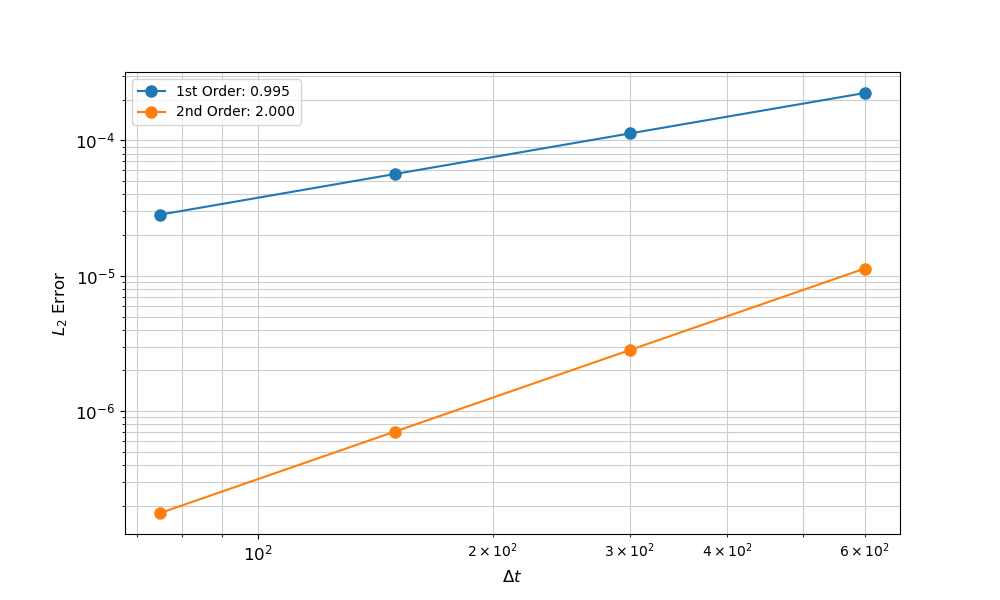
Figure 3: Results of the temporal convergence study comparing the finite element simulation with the assumed two-dimensional solution.
Closing Remarks
The above example demonstrates that a convergence study may be performed on simulations without a known solution by manufacturing a solution. Performing a convergence study is crucial to building robust simulation tools, as such a python package is provided to aid in performing the analysis.