FEM Convergence

Introduction

The temporal numerical integration methods as well as the FEM have known rates of convergence to the exact solution for changes in the time step and element size. The rates are exploited to verify that a simulation is performing as expected. The known convergence rates and the associated theory are well documented—e.g., Fish and Belytschko (2007)—the reader is encouraged to research the theory behind these rates. The following sections briefly discuss the known convergence rates.

Error Source

For a typical FEM simulation there are two primary sources of error: (1) error from the FEM approximation and (2) error from the time integration. Of course, there are other source of error such as floating point arithmetic and model simplifications. In the first case, the error associated with the FEM approximation goes to zero as the element size goes to zero. Similarly, as the time step in the numerical integration goes to zero so does the associated error.

Spatial Convergence

Spatial convergence for the FEM is defined here as the rate of error reduction with decreasing finite element size. The rate is dependent on the order of the shape functions and is typically reported as the slope of a line that compares error (y-axis) and element size (x-axis) on a log-log plot. First-order shape functions should have a slope of two and second-order a slope of three. For example, Figure 1, is an example convergence plot for a simulation with first-order and second-order shape functions, where the computed error is the norm.

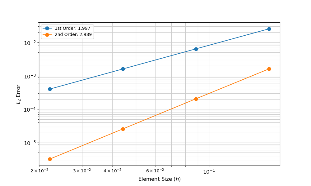
Figure 1: Example results for spatial convergence study.

Temporal Convergence

Temporal convergence is defined here as the rate of error reduction with decreasing the time step size. The rate is proportional to the order of the numerical integration scheme selected and typically reported as the slope of a line that compares the error (y-axis) and time step size (x-axis) on a log-log plot. This slope is expected to be one for first-order schemes, two for second-order schemes, etc. For example, Figure 2, is an example convergence plot for a simulation with first-order and second-order time integration schemes, where the computed error is the norm.

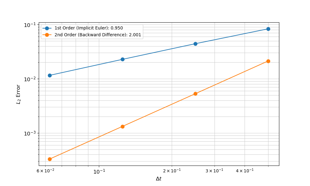
Figure 2: Example results for temporal convergence study.

References