General Case Description

This verification problem is taken from Longhurst et al. (1992) and Ambrosek and Longhurst (2008), and it has been updated and extended in Simon et al. (2025). In this problem, a composite structure of PyC and SiC is modeled with a constant concentration boundary condition of the free surface of PyC and zero concentration boundary condition on the free surface of the SiC.

Analytical solution at steady state

The steady state solution for the PyC is given in Longhurst et al. (1992) and Ambrosek and Longhurst (2008) as:

(1)

while the concentration profile for the SiC layer is given as:

(2)

where

= distance from free surface of PyC

= thickness of the PyC layer (33 m)

= thickness of the SiC layer (63 m in TMAP4 verification case, and 66 m in TMAP7 verification case)

= concentration at the PyC free surface (50.7079 moles/m)

= diffusivity in PyC (1.274 10 m/s)

= diffusivity in SiC (2.622 10 m/sec)

Analytical solution during transient

The analytical transient solution from Table 3, row 1 in Li and Cleall (2010) for the concentration in the PyC and SiC side of the composite slab is given as:

(3)

and

(4)

where

and are the roots of

(5)

Results

Figure 1 shows the comparison of the TMAP8 calculation and the analytical solution for concentration after steady-state is reached. The plots show the TMAP8 and analytical solution comparisons for both the TMAP4 case ( = 63 m) and the TMAP7 case ( = 66 m).

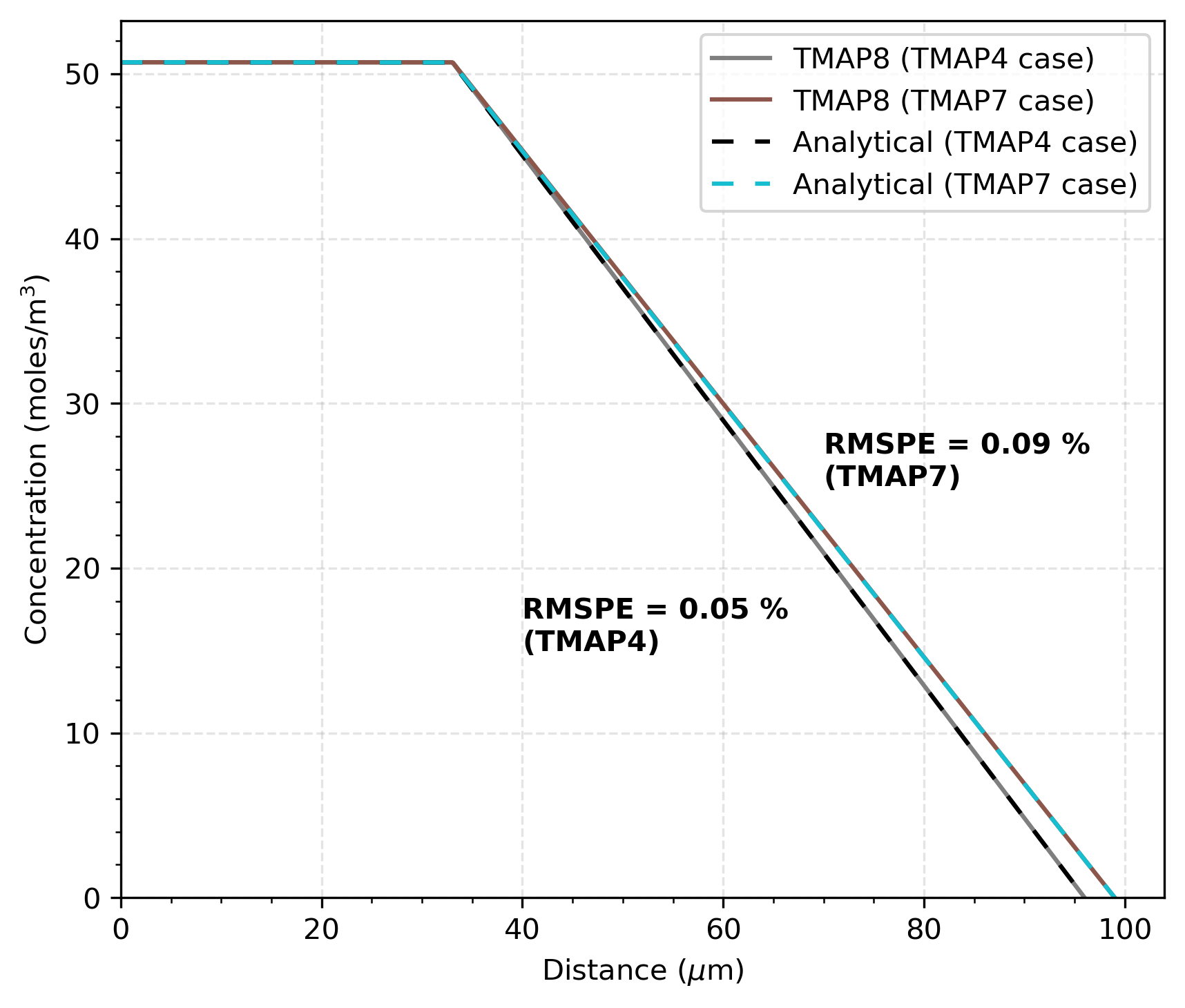
Figure 1: Comparison of TMAP8 calculation with the analytical solution at steady state. Bold text next to the plot curves shows the root mean square percentage error (RMSPE) between the TMAP8 prediction and analytical solution for the TMAP4 and TMAP7 verification cases.

For transient solution comparisons, we select two different points: One in the PyC layer at m, and one in the SiC layer. The concentration at these two points is calculated using TMAP8 and with the analytical equations (Eq. (3) and Eq. (4)). Figure 2 shows the comparison of the TMAP8 calculation against the analytical solution for this transient case in the PyC layer from 0 s to 1 s. Note that we only use the parameters from TMAP7 because the trivial difference between TMAP4 and TMAP7 in PyC layer. Figure 3 shows the comparison of the TMAP8 calculation against the analytical solution in the SiC layer. In the TMAP4 case, = 41 m, and in the TMAP7 case, = 48.75 m. There is good agreement between TMAP8 and the analytical solution for both steady state as well as transient cases. In both cases, the root mean square percentage error (RMSPE) is under 0.2%.

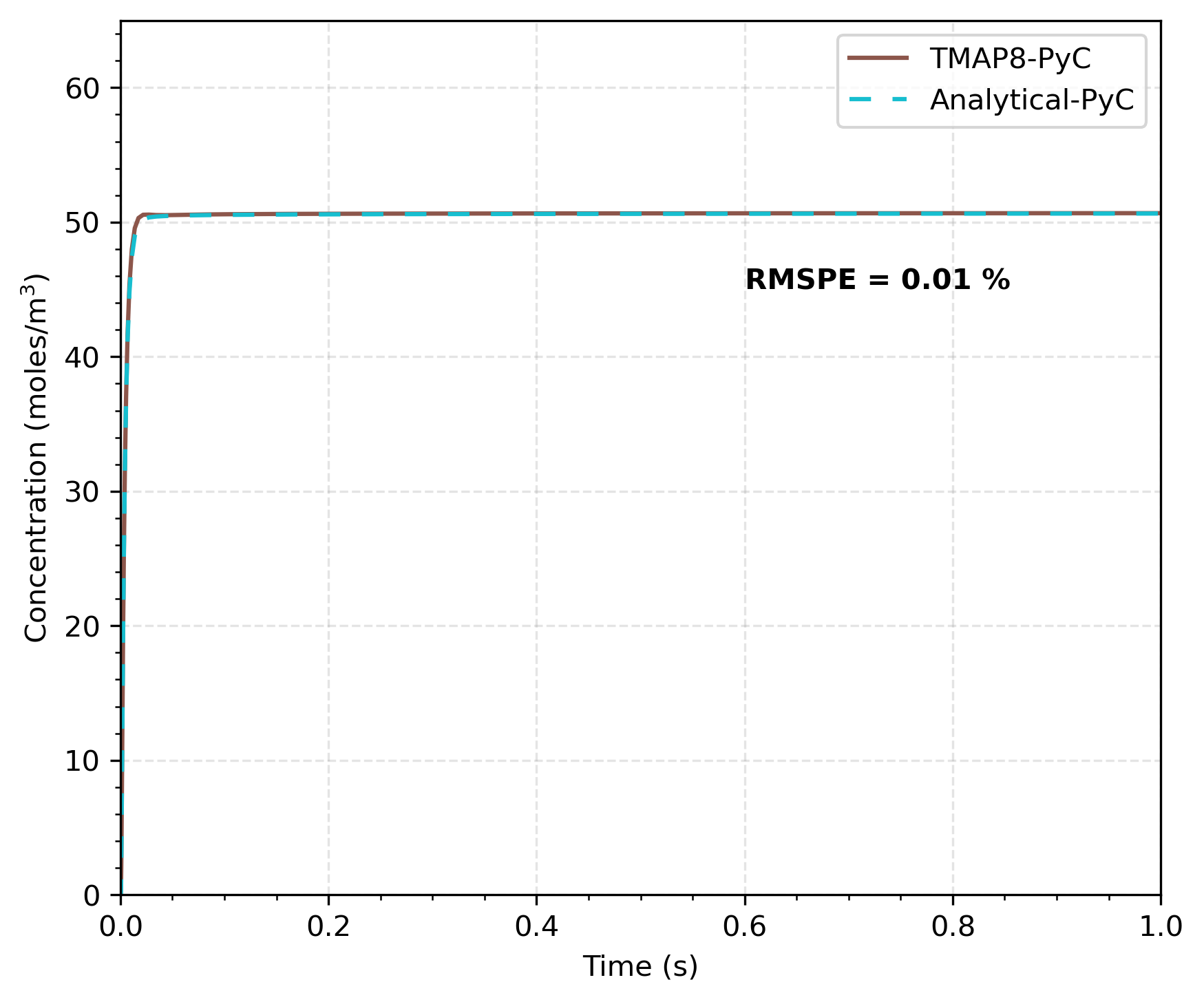
Figure 2: Comparison of TMAP8 calculation with the analytical solution at m in PyC layer. Bold text next to the plot curves shows the RMSPE for the match between the TMAP8 prediction and analytical solution for the TMAP4 and TMAP7 verification cases.

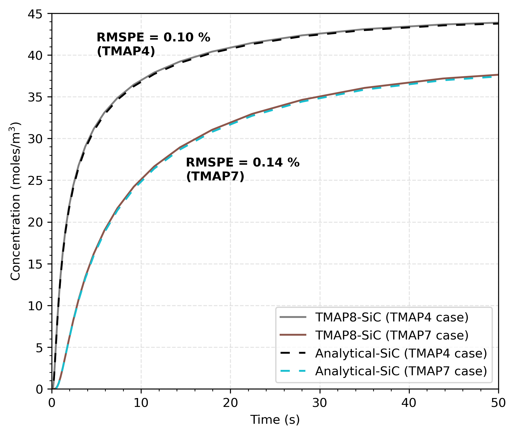
Figure 3: Comparison of TMAP8 calculation with the analytical solution in SiC layer. The compared distances are = 41 m in the TMAP4 case and = 48.75 m in the TMAP7 case. Bold text next to the plot curves shows the RMSPE for the match between the TMAP8 prediction and analytical solution for the TMAP4 and TMAP7 verification cases.

The error is calculated between the TMAP8 and analytical solution values after = 0.2 s. This is in order to ignore the unphysical predictions of the analytical solution at very small times as shown in Figure 4, which is a close-up view of Figure 3 close to the start of the simulation. The departure from physical results at low is due to the limited number of values being used from Eq. (5). We use the values from 0 to 100 in this case. The values in larger range will only have limited improvement in the accuracy but increase the running time for the computation of the analytical solutions.

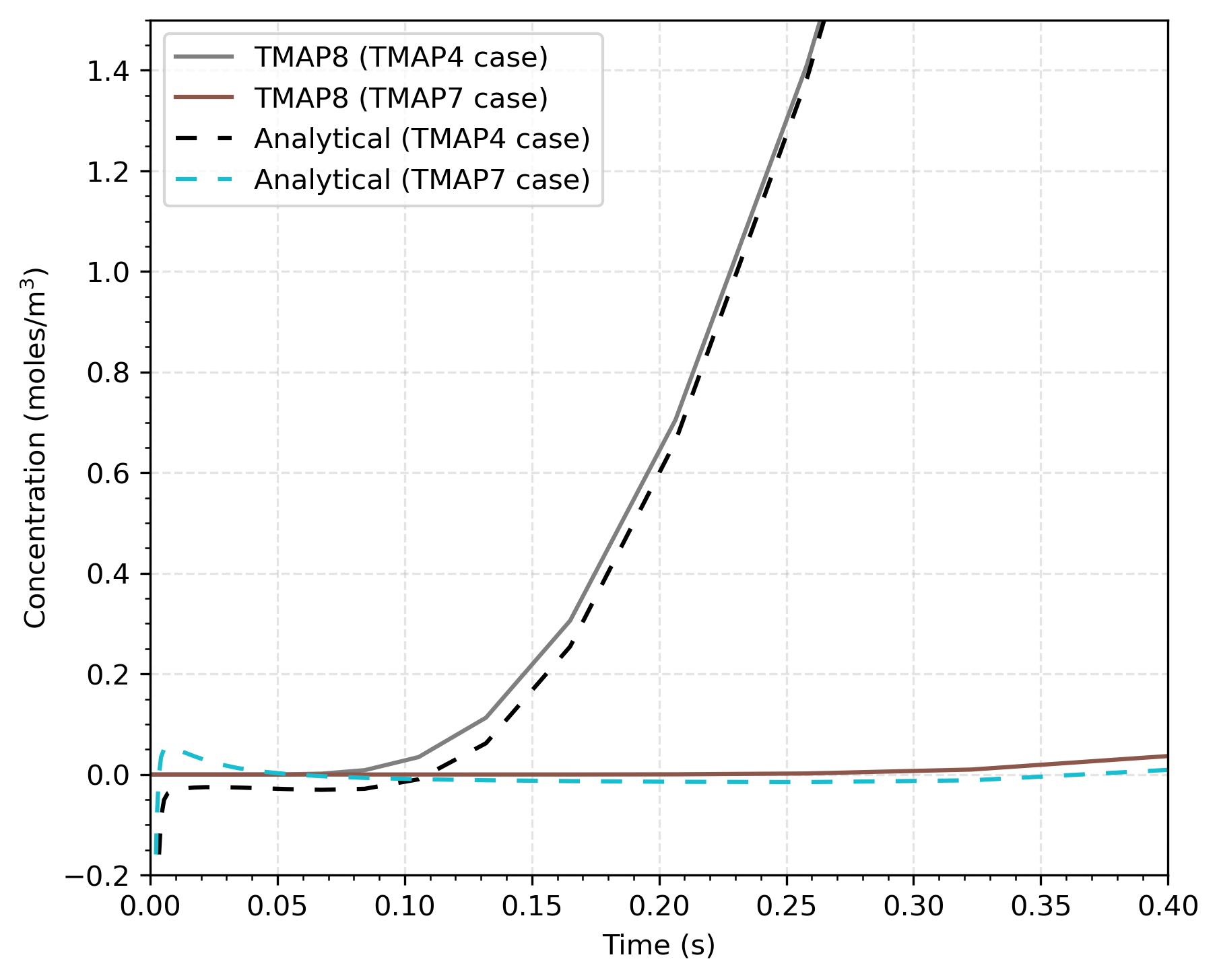
Figure 4: Zoomed-in view of comparison of TMAP8 calculation with the analytical solution for < 0.4 s. The analytical solution shows unphysical predictions close to = 0 s, whereas TMAP8's predictions are reasonable.

Input files

References