Comparison of surrogates using a time-dependent problem
This example is meant to demonstrate how non-intrusive surrogate models can be generated for time-dependent problems. Nearest Point, Polynomial Regression and Polynomial Chaos Expansion Surrogates are compared on a non-linear diffusion problem with an oscillating source.
Overview
In this case, a time-dependent nonlinear diffusion problem is solved on a square with an oscillating source in the center. The geometry is presented in Figure 1. It consists of a square with a source region in the center. The boundaries of the problem are denoted by . The strong formulation of the problem is:
(1)(2)where is temperature, and is a selection function returning 1 when and 0 otherwise. Parameters and influence the magnitude of the diffusion coefficient and the oscillation frequency of the source. Furthermore, it is assumed that the system is initially (at ) at constant temperature, . The uncertain parameters in the this problem are , and . A reference solution for the first of the transient is presented in Figure 2.
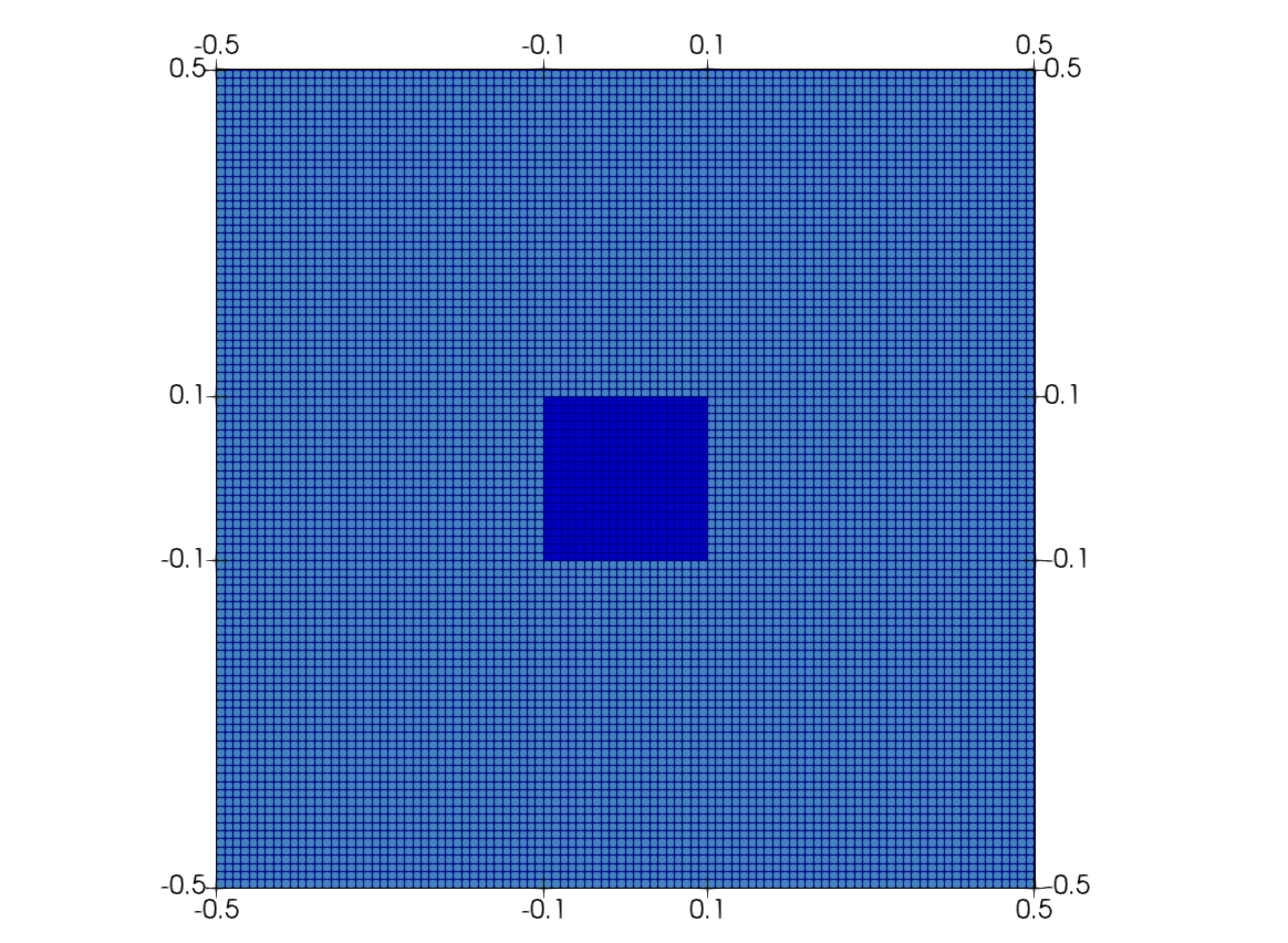
Figure 1: The geometry of the problem.

Figure 2: Reference solution for the problem.
In this problem the Quantities of Interest (QoIs) are the minimum and maximum temperatures in the domain over the fist of the transient:
(3)The uncertain parameters are assumed to be uniformly distributed between their corresponding minimum () and maximum () values:
| Parameter | Symbol | Distribution |
|---|---|---|
| Diffusion coefficient multiplier | ||
| Frequency multiplier | ||
| Initial temperature |
Solving the problem without uncertain parameters
The first step towards creating surrogate models is the generation of a full-order model which can solve Eq. (1) with fixed parameter combinations. The complete input file for this case is presented in Listing 1. It is visible that a mesh and timestep is used to solve the transient problem.
Listing 1: Complete input file for the time-dependent heat equation problem in this study.
[Functions<<<{"href": "../../../syntax/Functions/index.html"}>>>]
  [src_func]
    type = ParsedFunction<<<{"description": "Function created by parsing a string", "href": "../../../source/functions/MooseParsedFunction.html"}>>>
    expression<<<{"description": "The user defined function."}>>> = "1000*sin(f*t)"
    symbol_names<<<{"description": "Symbols (excluding t,x,y,z) that are bound to the values provided by the corresponding items in the vals vector."}>>> = 'f'
    symbol_values<<<{"description": "Constant numeric values, postprocessor names, function names, and scalar variables corresponding to the symbols in symbol_names."}>>> = '20'
  []
[]

[Mesh<<<{"href": "../../../syntax/Mesh/index.html"}>>>]
  [msh]
    type = GeneratedMeshGenerator<<<{"description": "Create a line, square, or cube mesh with uniformly spaced or biased elements.", "href": "../../../source/meshgenerators/GeneratedMeshGenerator.html"}>>>
    dim<<<{"description": "The dimension of the mesh to be generated"}>>> = 2
    nx<<<{"description": "Number of elements in the X direction"}>>> = 100
    xmin<<<{"description": "Lower X Coordinate of the generated mesh"}>>> = -0.5
    xmax<<<{"description": "Upper X Coordinate of the generated mesh"}>>> = 0.5
    ny<<<{"description": "Number of elements in the Y direction"}>>> = 100
    ymin<<<{"description": "Lower Y Coordinate of the generated mesh"}>>> = -0.5
    ymax<<<{"description": "Upper Y Coordinate of the generated mesh"}>>> = 0.5
  []
  [source_domain]
    type = ParsedSubdomainMeshGenerator<<<{"description": "Uses a parsed expression (`combinatorial_geometry`) to determine if an element (via its centroid) is inside the region defined by the expression and assigns a new block ID.", "href": "../../../source/meshgenerators/ParsedSubdomainMeshGenerator.html"}>>>
    input<<<{"description": "The mesh we want to modify"}>>> = msh
    combinatorial_geometry<<<{"description": "Function expression encoding a combinatorial geometry"}>>> = '(x<0.1 & x>-0.1) & (y<0.1 & y>-0.1)'
    block_id<<<{"description": "Subdomain id to set for inside of the combinatorial"}>>>=1
  []
[]

[Variables<<<{"href": "../../../syntax/Variables/index.html"}>>>]
  [T]
    initial_condition<<<{"description": "Specifies a constant initial condition for this variable"}>>> = 300
  []
[]

[Kernels<<<{"href": "../../../syntax/Kernels/index.html"}>>>]
  [diffusion]
    type = MatDiffusion<<<{"description": "Diffusion equation Kernel that takes an isotropic Diffusivity from a material property", "href": "../../../source/kernels/MatDiffusion.html"}>>>
    variable<<<{"description": "The name of the variable that this residual object operates on"}>>> = T
    diffusivity<<<{"description": "The diffusivity value or material property"}>>> = diff_coeff
  []
  [source]
    type = BodyForce<<<{"description": "Demonstrates the multiple ways that scalar values can be introduced into kernels, e.g. (controllable) constants, functions, and postprocessors. Implements the weak form $(\\psi_i, -f)$.", "href": "../../../source/kernels/BodyForce.html"}>>>
    variable<<<{"description": "The name of the variable that this residual object operates on"}>>> = T
    function<<<{"description": "A function that describes the body force"}>>> = src_func
    block<<<{"description": "The list of blocks (ids or names) that this object will be applied"}>>> = 1
  []
  [time_deriv]
    type = TimeDerivative<<<{"description": "The time derivative operator with the weak form of $(\\psi_i, \\frac{\\partial u_h}{\\partial t})$.", "href": "../../../source/kernels/TimeDerivative.html"}>>>
    variable<<<{"description": "The name of the variable that this residual object operates on"}>>> = T
  []
[]

[Materials<<<{"href": "../../../syntax/Materials/index.html"}>>>]
  [diff_coeff]
    type = ParsedMaterial<<<{"description": "Parsed expression Material.", "href": "../../../source/materials/ParsedMaterial.html"}>>>
    property_name<<<{"description": "Name of the parsed material property"}>>> = diff_coeff
    coupled_variables<<<{"description": "Vector of variables used in the parsed function"}>>> = 'T'
    constant_names<<<{"description": "Vector of constants used in the parsed function (use this for kB etc.)"}>>> = 'C'
    constant_expressions<<<{"description": "Vector of values for the constants in constant_names (can be an FParser expression)"}>>> = 0.02
    expression<<<{"description": "Parsed function (see FParser) expression for the parsed material"}>>> = 'C * pow(300/T, 2)'
  []
[]

[BCs<<<{"href": "../../../syntax/BCs/index.html"}>>>]
  [neumann_all]
    type = NeumannBC<<<{"description": "Imposes the integrated boundary condition $\\frac{\\partial u}{\\partial n}=h$, where $h$ is a constant, controllable value.", "href": "../../../source/bcs/NeumannBC.html"}>>>
    variable<<<{"description": "The name of the variable that this residual object operates on"}>>> = T
    boundary<<<{"description": "The list of boundary IDs from the mesh where this object applies"}>>> = 'left right top bottom'
    value<<<{"description": "For a Laplacian problem, the value of the gradient dotted with the normals on the boundary."}>>> = 0
  []
[]

[Executioner<<<{"href": "../../../syntax/Executioner/index.html"}>>>]
  type = Transient
  num_steps = 100
  dt = 0.01
  solve_type = PJFNK
  petsc_options_iname = '-pc_type -pc_hypre_type'
  petsc_options_value = 'hypre boomeramg'
  nl_rel_tol = 1e-6
  l_abs_tol = 1e-6
  timestep_tolerance = 1e-6
[]

[Postprocessors<<<{"href": "../../../syntax/Postprocessors/index.html"}>>>]
  [max]
    type = NodalExtremeValue<<<{"description": "Finds either the min or max elemental value of a variable over the domain.", "href": "../../../source/postprocessors/NodalExtremeValue.html"}>>>
    variable<<<{"description": "The name of the variable that this postprocessor operates on"}>>> = T
  []
  [min]
    type = NodalExtremeValue<<<{"description": "Finds either the min or max elemental value of a variable over the domain.", "href": "../../../source/postprocessors/NodalExtremeValue.html"}>>>
    variable<<<{"description": "The name of the variable that this postprocessor operates on"}>>> = T
    value_type<<<{"description": "Type of extreme value to return. 'max' returns the maximum value. 'min' returns the minimum value. 'max_abs' returns the maximum of the absolute value."}>>> = min
  []
  [time_max]
    type = TimeExtremeValue<<<{"description": "A postprocessor for reporting the extreme value of another postprocessor over time.", "href": "../../../source/postprocessors/TimeExtremeValue.html"}>>>
    postprocessor<<<{"description": "The name of the postprocessor used for reporting time extreme values"}>>> = max
  []
  [time_min]
    type = TimeExtremeValue<<<{"description": "A postprocessor for reporting the extreme value of another postprocessor over time.", "href": "../../../source/postprocessors/TimeExtremeValue.html"}>>>
    postprocessor<<<{"description": "The name of the postprocessor used for reporting time extreme values"}>>> = min
    value_type<<<{"description": "Type of extreme value to return.'max' returns the maximum value.'min' returns the minimum value.'abs_max' returns the maximum absolute value.'abs_min' returns the minimum absolute value."}>>> = min
  []
[]Training surrogate models
This problem involves the generation of three surrogates: a NearestPointSurrogate, a PolynomialRegressionSurrogate and a PolynomialChaos. All three of them are constructed using multiple instances of the full-order problem as sub-applications. This step is managed by a trainer input file which is responsible for creating parameter samples, transferring those to sub-applications and collecting the corresponding results. The reader is recommended to read Training a Surrogate Model and Parameter Study to get a clear picture on how to train and set up a surrogate model.
The training phase starts with the definition of the distributions for the uncertain parameters in the Distributions block. The uniform distributions can be defined as:
[Distributions<<<{"href": "../../../syntax/Distributions/index.html"}>>>]
  [C_dist]
    type = Uniform<<<{"description": "Continuous uniform distribution.", "href": "../../../source/distributions/Uniform.html"}>>>
    lower_bound<<<{"description": "Distribution lower bound"}>>> = 0.01
    upper_bound<<<{"description": "Distribution upper bound"}>>> = 0.02
  []
  [f_dist]
    type = Uniform<<<{"description": "Continuous uniform distribution.", "href": "../../../source/distributions/Uniform.html"}>>>
    lower_bound<<<{"description": "Distribution lower bound"}>>> = 15
    upper_bound<<<{"description": "Distribution upper bound"}>>> = 25
  []
  [init_dist]
    type = Uniform<<<{"description": "Continuous uniform distribution.", "href": "../../../source/distributions/Uniform.html"}>>>
    lower_bound<<<{"description": "Distribution lower bound"}>>> = 270
    upper_bound<<<{"description": "Distribution upper bound"}>>> = 330
  []
[]Next, multiple parameter vectors are prepared by sampling the underlying distributions using the objects in the Samplers block. In this case, the samples are generated by a QuadratureSampler, which is optimal for the polynomial chaos expansion. Since the execution of this example is expensive in terms of computation time, the same samples are used to train the other surrogates as well. It is not visible, but the sampler prepares 216 parameter vectors altogether.
[Samplers<<<{"href": "../../../syntax/Samplers/index.html"}>>>]
  [sample]
    type = Quadrature<<<{"description": "Quadrature sampler for Polynomial Chaos.", "href": "../../../source/samplers/QuadratureSampler.html"}>>>
    order<<<{"description": "Specify the maximum order of the polynomials in the expansion."}>>> = 5
    distributions<<<{"description": "The distribution names to be sampled, the number of distributions provided defines the number of columns per matrix and their type defines the quadrature."}>>> = 'C_dist f_dist init_dist'
    execute_on<<<{"description": "The list of flag(s) indicating when this object should be executed. For a description of each flag, see https://mooseframework.inl.gov/source/interfaces/SetupInterface.html."}>>> = PRE_MULTIAPP_SETUP
  []
[]The objects in blocks Controls, MultiApps, Transfers and Reporters are responsible for managing the communication between the trainer and sub-applications, execution of the sub-applications and the collection of the results. For a more detailed description of these blocks see Parameter Study and Training a Surrogate Model.
[MultiApps<<<{"href": "../../../syntax/MultiApps/index.html"}>>>]
  [runner]
    type = SamplerFullSolveMultiApp<<<{"description": "Creates a full-solve type sub-application for each row of each Sampler matrix.", "href": "../../../source/multiapps/SamplerFullSolveMultiApp.html"}>>>
    input_files<<<{"description": "The input file for each App.  If this parameter only contains one input file it will be used for all of the Apps.  When using 'positions_from_file' it is also admissable to provide one input_file per file."}>>> = 'trans_diff_sub.i'
    sampler<<<{"description": "The Sampler object to utilize for creating MultiApps."}>>> = sample
  []
[]

[Controls<<<{"href": "../../../syntax/Controls/index.html"}>>>]
  [cmdline]
    type = MultiAppSamplerControl<<<{"description": "Control for modifying the command line arguments of MultiApps.", "href": "../../../source/controls/MultiAppSamplerControl.html"}>>>
    multi_app<<<{"description": "The name of the MultiApp to control."}>>> = runner
    sampler<<<{"description": "The Sampler object to utilize for altering the command line options of the MultiApp."}>>> = sample
    param_names<<<{"description": "The names of the command line parameters to set via the sampled data."}>>> = 'Materials/diff_coeff/constant_expressions Functions/src_func/vals Variables/T/initial_condition'
  []
[]

[Transfers<<<{"href": "../../../syntax/Transfers/index.html"}>>>]
  [results]
    type = SamplerReporterTransfer<<<{"description": "Transfers data from Reporters on the sub-application to a StochasticReporter on the main application.", "href": "../../../source/transfers/SamplerReporterTransfer.html"}>>>
    from_multi_app<<<{"description": "The name of the MultiApp to receive data from"}>>> = runner
    sampler<<<{"description": "A the Sampler object that Transfer is associated.."}>>> = sample
    stochastic_reporter<<<{"description": "The name of the StochasticReporter object to transfer values to."}>>> = trainer_results
    from_reporter<<<{"description": "The name(s) of the Reporter(s) on the sub-app to transfer from."}>>> = 'time_max/value time_min/value'
  []
[]

[Reporters<<<{"href": "../../../syntax/Reporters/index.html"}>>>]
  [trainer_results]
    type = StochasticReporter<<<{"description": "Storage container for stochastic simulation results coming from Reporters.", "href": "../../../source/reporters/StochasticReporter.html"}>>>
  []
[]Next, six trainers (three different surrogates for each QoI) are defined in the Trainers block. These objects use the data from Samplers and Reporters. A polynomial chaos surrogate of order 5, a polynomial regression surrogate with a polynomial of degree at most 4 and a nearest point surrogate is used for both QoIs in this work. The PolynomialChaosTrainer also needs knowledge about the underlying parameter distributions to be able to select appropriate polynomials.
[Trainers<<<{"href": "../../../syntax/Trainers/index.html"}>>>]
  [pc_max]
    type = PolynomialChaosTrainer<<<{"description": "Computes and evaluates polynomial chaos surrogate model.", "href": "../../../source/trainers/PolynomialChaosTrainer.html"}>>>
    execute_on<<<{"description": "The list of flag(s) indicating when this object should be executed. For a description of each flag, see https://mooseframework.inl.gov/source/interfaces/SetupInterface.html."}>>> = final
    order<<<{"description": "Maximum polynomial order."}>>> = 5
    distributions<<<{"description": "Names of the distributions samples were taken from."}>>> = 'C_dist f_dist init_dist'
    sampler<<<{"description": "Sampler used to create predictor and response data."}>>> = sample
    response<<<{"description": "Reporter value of response results, can be vpp with <vpp_name>/<vector_name> or sampler column with 'sampler/col_<index>'."}>>> = trainer_results/results:time_max:value
  []
  [pc_min]
    type = PolynomialChaosTrainer<<<{"description": "Computes and evaluates polynomial chaos surrogate model.", "href": "../../../source/trainers/PolynomialChaosTrainer.html"}>>>
    execute_on<<<{"description": "The list of flag(s) indicating when this object should be executed. For a description of each flag, see https://mooseframework.inl.gov/source/interfaces/SetupInterface.html."}>>> = final
    order<<<{"description": "Maximum polynomial order."}>>> = 5
    distributions<<<{"description": "Names of the distributions samples were taken from."}>>> = 'C_dist f_dist init_dist'
    sampler<<<{"description": "Sampler used to create predictor and response data."}>>> = sample
    response<<<{"description": "Reporter value of response results, can be vpp with <vpp_name>/<vector_name> or sampler column with 'sampler/col_<index>'."}>>> = trainer_results/results:time_min:value
  []
  [np_max]
    type = NearestPointTrainer<<<{"description": "Loops over and saves sample values for [NearestPointSurrogate.md].", "href": "../../../source/trainers/NearestPointTrainer.html"}>>>
    execute_on<<<{"description": "The list of flag(s) indicating when this object should be executed. For a description of each flag, see https://mooseframework.inl.gov/source/interfaces/SetupInterface.html."}>>> = final
    sampler<<<{"description": "Sampler used to create predictor and response data."}>>> = sample
    response<<<{"description": "Reporter value of response results, can be vpp with <vpp_name>/<vector_name> or sampler column with 'sampler/col_<index>'."}>>> = trainer_results/results:time_max:value
  []
  [np_min]
    type = NearestPointTrainer<<<{"description": "Loops over and saves sample values for [NearestPointSurrogate.md].", "href": "../../../source/trainers/NearestPointTrainer.html"}>>>
    execute_on<<<{"description": "The list of flag(s) indicating when this object should be executed. For a description of each flag, see https://mooseframework.inl.gov/source/interfaces/SetupInterface.html."}>>> = final
    sampler<<<{"description": "Sampler used to create predictor and response data."}>>> = sample
    response<<<{"description": "Reporter value of response results, can be vpp with <vpp_name>/<vector_name> or sampler column with 'sampler/col_<index>'."}>>> = trainer_results/results:time_min:value
  []
  [pr_max]
    type = PolynomialRegressionTrainer<<<{"description": "Computes coefficients for polynomial regession model.", "href": "../../../source/trainers/PolynomialRegressionTrainer.html"}>>>
    regression_type<<<{"description": "The type of regression to perform."}>>> = "ols"
    execute_on<<<{"description": "The list of flag(s) indicating when this object should be executed. For a description of each flag, see https://mooseframework.inl.gov/source/interfaces/SetupInterface.html."}>>> = final
    max_degree<<<{"description": "Maximum polynomial degree to use for the regression."}>>> = 4
    sampler<<<{"description": "Sampler used to create predictor and response data."}>>> = sample
    response<<<{"description": "Reporter value of response results, can be vpp with <vpp_name>/<vector_name> or sampler column with 'sampler/col_<index>'."}>>> = trainer_results/results:time_max:value
  []
  [pr_min]
    type = PolynomialRegressionTrainer<<<{"description": "Computes coefficients for polynomial regession model.", "href": "../../../source/trainers/PolynomialRegressionTrainer.html"}>>>
    regression_type<<<{"description": "The type of regression to perform."}>>> = "ols"
    execute_on<<<{"description": "The list of flag(s) indicating when this object should be executed. For a description of each flag, see https://mooseframework.inl.gov/source/interfaces/SetupInterface.html."}>>> = final
    max_degree<<<{"description": "Maximum polynomial degree to use for the regression."}>>> = 4
    sampler<<<{"description": "Sampler used to create predictor and response data."}>>> = sample
    response<<<{"description": "Reporter value of response results, can be vpp with <vpp_name>/<vector_name> or sampler column with 'sampler/col_<index>'."}>>> = trainer_results/results:time_min:value
  []
[]As a last step in the training process, the important parameters of the trained surrogates are saved into restartable data files, which can be used to construct the surrogate models again without repeating the training process.
[Outputs<<<{"href": "../../../syntax/Outputs/index.html"}>>>]
  [out]
    type = SurrogateTrainerOutput<<<{"description": "Output for trained surrogate model data.", "href": "../../../source/outputs/SurrogateTrainerOutput.html"}>>>
    trainers<<<{"description": "A list of SurrogateTrainer objects to output."}>>> = 'pc_max pc_min np_max np_min pr_max pr_min'
    execute_on<<<{"description": "The list of flag(s) indicating when this object should be executed. For a description of each flag, see https://mooseframework.inl.gov/source/interfaces/SetupInterface.html."}>>> = FINAL
  []
[]Evaluation of surrogate models
A new main input file has been created to evaluate the surrogate models. This input file uses the same parameter distribution as the one used for the training of the surrogates. Each surrogate model is tested using a new, test parameter sample set, which is generated using a LatinHypercube object in the Samplers block. Since the surrogate models are orders of magnitude faster, samples are prepared for testing (compared to used for training).
[Samplers<<<{"href": "../../../syntax/Samplers/index.html"}>>>]
  [sample]
    type = LatinHypercube<<<{"description": "Latin Hypercube Sampler.", "href": "../../../source/samplers/LatinHypercubeSampler.html"}>>>
    num_rows<<<{"description": "The size of the square matrix to generate."}>>> = 100000
    distributions<<<{"description": "The distribution names to be sampled, the number of distributions provided defines the number of columns per matrix."}>>> = 'C_dist f_dist init_dist'
    execute_on<<<{"description": "The list of flag(s) indicating when this object should be executed. For a description of each flag, see https://mooseframework.inl.gov/source/interfaces/SetupInterface.html."}>>> = PRE_MULTIAPP_SETUP
  []
[]Next, the necessary objects are created in the Surrogates block using the information available within the corresponding restartable data files.
[Surrogates<<<{"href": "../../../syntax/Surrogates/index.html"}>>>]
  [pc_min]
    type = PolynomialChaos<<<{"description": "Computes and evaluates polynomial chaos surrogate model.", "href": "../../../source/surrogates/PolynomialChaos.html"}>>>
    filename<<<{"description": "The name of the file which will be associated with the saved/loaded data."}>>> = 'trans_diff_trainer_out_pc_min.rd'
  []
  [pc_max]
    type = PolynomialChaos<<<{"description": "Computes and evaluates polynomial chaos surrogate model.", "href": "../../../source/surrogates/PolynomialChaos.html"}>>>
    filename<<<{"description": "The name of the file which will be associated with the saved/loaded data."}>>> = 'trans_diff_trainer_out_pc_max.rd'
  []
  [pr_min]
    type = PolynomialRegressionSurrogate<<<{"description": "Evaluates polynomial regression model with coefficients computed from PolynomialRegressionTrainer.", "href": "../../../source/surrogates/PolynomialRegressionSurrogate.html"}>>>
    filename<<<{"description": "The name of the file which will be associated with the saved/loaded data."}>>> = 'trans_diff_trainer_out_pr_min.rd'
  []
  [pr_max]
    type = PolynomialRegressionSurrogate<<<{"description": "Evaluates polynomial regression model with coefficients computed from PolynomialRegressionTrainer.", "href": "../../../source/surrogates/PolynomialRegressionSurrogate.html"}>>>
    filename<<<{"description": "The name of the file which will be associated with the saved/loaded data."}>>> = 'trans_diff_trainer_out_pr_max.rd'
  []
  [np_min]
    type = NearestPointSurrogate<<<{"description": "Surrogate that evaluates the value from the nearest point from data in [NearestPointTrainer.md]", "href": "../../../source/surrogates/NearestPointSurrogate.html"}>>>
    filename<<<{"description": "The name of the file which will be associated with the saved/loaded data."}>>> = 'trans_diff_trainer_out_np_min.rd'
  []
  [np_max]
    type = NearestPointSurrogate<<<{"description": "Surrogate that evaluates the value from the nearest point from data in [NearestPointTrainer.md]", "href": "../../../source/surrogates/NearestPointSurrogate.html"}>>>
    filename<<<{"description": "The name of the file which will be associated with the saved/loaded data."}>>> = 'trans_diff_trainer_out_np_max.rd'
  []
[]These surrogate models are then evaluated at the points defined in the testing sample batch. This is done using objects in the Reporters block. Furthermore, the mean values and standard deviations of the QoI-s together with the confidence intervals are generated as well.
[Reporters<<<{"href": "../../../syntax/Reporters/index.html"}>>>]
  [eval_surr]
    type = EvaluateSurrogate<<<{"description": "Tool for sampling surrogate models.", "href": "../../../source/reporters/EvaluateSurrogate.html"}>>>
    model<<<{"description": "Name of surrogate models."}>>> = 'pc_max pc_min pr_max pr_min np_max np_min'
    sampler<<<{"description": "Sampler to use for evaluating surrogate models."}>>> = sample
    parallel_type<<<{"description": "This parameter will determine how the stochastic data is gathered. It is common for outputting purposes that this parameter be set to ROOT, otherwise, many files will be produced showing the values on each processor. However, if there are lot of samples, gathering on root may be memory restrictive."}>>> = ROOT
  []
  [eval_surr_stats]
    type = StatisticsReporter<<<{"description": "Compute statistical values of a given VectorPostprocessor objects and vectors.", "href": "../../../source/reporters/StatisticsReporter.html"}>>>
    reporters<<<{"description": "List of Reporter values to utilized for statistic computations."}>>> = 'eval_surr/pc_max eval_surr/pc_min eval_surr/pr_max eval_surr/pr_min eval_surr/np_max eval_surr/np_min'
    compute<<<{"description": "The statistic(s) to compute for each of the supplied vector postprocessors."}>>> = 'mean stddev'
    ci_method<<<{"description": "The method to use for computing confidence level intervals."}>>> = 'percentile'
    ci_levels<<<{"description": "A vector of confidence levels to consider, values must be in (0, 1)."}>>> = '0.05 0.95'
  []
[]Results and Analysis
In this section the results from the different surrogate models are provided. Additionally, the full-order model has been tested with a 2,000 sample batch to serve as a reference solution. The main input file for testing with the full-order model is available here. A short analysis of the results is provided as well.
First, the distributions of QoI-s from the surrogates are compared to the reference results. The histograms showing the distribution of the maximum temperature through the transient are presented below. The figures can be enlarged by clicking on them.

Figure 3: Polynomial Chaos Expansion Surrogate.

Figure 4: Polynomial Regression Surrogate.

Figure 5: Nearest Point Surrogate.
It is visible that even with 2,000 samples, the reference results still exhibit a high statistical fluctuation. Unfortunately, having considerably more than 2,000 samples using the full-order model is not efficient due to the extremely long simulation time. It is also visible that both the polynomial chaos and polynomial regression surrogates yield approximately the same results, and with 100,000 samples, the distributions are much smoother. On the other hand, the nearest point surrogate introduces additional fluctuations which means that it is not capable of reconstructing the shape of the original distribution at all. The same phenomena is experienced with the minimum temperature. The corresponding histograms are presented below.

Figure 6: Polynomial Chaos Expansion Surrogate.

Figure 7: Polynomial Regression Surrogate.

Figure 8: Nearest Point Surrogate.
Next, the statistical moments are compared in Table 1 for the maximum temperature and in Table 2 for the minimum temperature of the system.
Table 1: The mean and standard deviation of the maximum temperature obtained using the surrogates and a reference full-order model.
| Model | Number of samples | Mean | 95% CI | Std. Dev. | 95% CI |
|---|---|---|---|---|---|
| Full-order model (reference) | 2,000 | 396.74 | [395.90, 397.58] | 22.86 | [22.36, 23.33] |
| Nearest Point Surrogate | 100,000 | 396.87 | [396.74, 396.99] | 23.57 | [23.50, 23.64] |
| Polynomial Chaos Surrogate | 100,000 | 396.77 | [396.65, 396.88] | 22.85 | [22.78, 22.92] |
| Polynomial Regression Surrogate | 100,000 | 396.77 | [396.65, 396.88] | 22.85 | [22.78, 22.93] |
Table 2: The mean and standard deviation of the minimum temperature obtained using the surrogates and a reference full-order model.
| Model | Number of samples | Mean | 95% CI | Std. Dev. | 95% CI |
|---|---|---|---|---|---|
| Full-order model (reference) | 2,000 | 260.66 | [259.94, 261.38] | 19.30 | [18.96, 19.64] |
| Nearest Point Surrogate | 100,000 | 260.46 | [260.36, 260.56] | 19.77 | [19.72, 19.82] |
| Polynomial Chaos Surrogate | 100,000 | 260.46 | [260.36, 260.56] | 19.17 | [19.12, 19.21] |
| Polynomial Regression Surrogate | 100,000 | 260.46 | [260.36, 260.56] | 19.17 | [19.12, 19.22] |
Even though there are small differences in the mean values, it can be concluded that all three of the surrogates managed to give the correct answer. The differences between the full-order model and surrogates are statistically insignificant. For the standard deviations, on the other hand, only the polynomial chaos and polynomial regression give back the statistically equivalent results. Lastly, the gain in computation time is presented in Table 3. It is important to mention that all of the results have been obtained using 8 cores of a single machine.
Table 3: The wall-clock times of different steps in the surrogate modeling process.
| Case | Wall-clock time (s) |
|---|---|
| Creating reference results (2000 samples) | 16,374.2 |
| Training surrogates | 1910.4 |
| Evaluating surrogates (without computing CI) | 1.6 |
| Evaluating surrogates (with computing CI) | 275.0 |
It is visible that training and using a surrogate model is beneficial in this case since it saves a considerable amount of computation time. It can also be observed that computing the confidence intervals for surrogate models is the most work intensive step in the testing phase. This is due to the frequent resampling of the results vectors.