Sodium Fast Reactor (SFR) Single Assembly Model
Contact: Nicholas Martin, nicolas.martin.at.inl.gov
Model link: SFR Single Assembly Model
SFR model description
This VTB model provides an example representative of a Sodium cooled Fast Reactor (SFR) using metallic fuel. Reactor core analyses of SFR require the modeling of multiple physics systems, such as:
Neutron flux distribution throughout the core, obtained by solving the neutron transport equation.
Coolant temperature and density distribution, obtained by solving the thermal-hydraulic equation system for the flowing sodium.
Fuel temperature distribution, obtained by solving the heat conduction equation in the fuel rods.
Due to the large temperature gradients occurring in SFR cores, thermal expansion plays a significant role and needs to be accounted for by computational models.
The proposed VTB multiphysics SFR model captures the predominant feedback mechanisms and consists of 4 independent application inputs:
A 3D Griffin neutronics model, whose main purpose is to compute the 3D neutron flux / power given the local field temperatures and mechanical deformations due to thermal expansion.
A 2D axisymmetric BISON model of the fuel rod which predicts the thermal response given a power density, as well as the thermal expansion occurring in the fuel/clad materials. The predicted quantities (fuel temperature, axial expansion in the fuel) are then passed back to the neutronics model. One BISON input is instantiated per fuel assembly.
A tensor mechanic input of the core support plate, predicting the stress-strain relationships given the inlet sodium temperature. The displacements are passed to the neutronics model to account for the radial displacements in the core geometry. Since the core support plate expansion is tied to the inlet temperature (fixed in this analysis), this model is only called once at the beginning of the simulation.
A SAM 1D channel input, whose purpose is to compute the coolant channel temperature / density profile and pressure drop, given the orifice strategy selected which dictates the input mass flow rate and outlet pressure and the wall temperature coming from the BISON thermal model. The coolant density and heat transfer coefficient is passed back to BISON to be used in a convective heat flux boundary condition. The coolant density is also passed back to the neutronics model for updating the cross sections. One SAM input is instantiated per coolant channel. The coupling scheme with the variables exchanged between solvers is given in Figure 1.
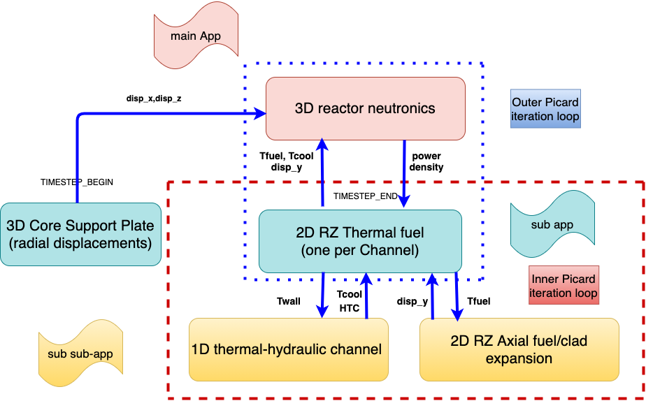
Figure 1: The coupling scheme used for the SFR model.
Note: this model consists of one single assembly in 3D, with reflective boundary conditions radially for the neutronics model so as to mimic an infinite domain in the X and Y directions, and void boundary conditions axially. A representative fuel rod is modeled with BISON where the power density generated by Griffin is normalized to correspond to the average pin power. The coolant channel is modeled via a 1D model in SAM. This example provides all the functionalities required for scaling up to a full 3D model without having to provide any proprietary fuel and core dimensions.
Griffin Model
Griffin geometry
The geometry used in this test case contains a single 3D assembly for the neutronics model, coupled with a single 2D RZ BISON model for the thermo-mechanical model, as well as a 1D thermal-hydraulic channel model. The dimensions are non proprietary and representative of past and current SFR designs. The fuel assembly pitch is 12 cm, with 217 pins. Axially, the fuel is composed of a bottom reflector, a fuel region, a plenum region to accommodate fission gas releases, and a top reflector. The reflector regions are assumed to be each one meter, and the fuel rod is 2 meters: one meter for the rodded part, and one meter for the plenum region, leading to a fuel assembly height of 4 meters. The assembly mesh is displayed in Figure 2. A 2D core support plate model is also provided with the corresponding dimensions.
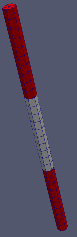
Figure 2: Mesh used for Griffin. Red indicates the bottom and top axial reflectors. White corresponds to the fuel region.
Griffin Cross Section Model for SFR
Cross sections for Griffin are provided for the 4 material required for this model (bottom reflector, fuel, plenum, top reflector). The cross sections are functionalized as a function of the fuel temperature, and coolant temperature. Note that material density changes, due to mesh displacements from the core support plate model and the BISON mechanical model are also captured by the neutronics cross sections and thus the results (Keff, flux). The cross section parametrization can be written using a functional formulation: Where f is approximated by a piece-wise linear function that uses the local parameter values at each element of the mesh coming from the other physics models. The grid selected for each parameter is: - . -
The maximum fuel temperature was selected to coincide with the value used for generating Doppler coefficient in the ARC reference calculation (1800 K), so as to avoid extrapolation. No changes in density was applied when varying the fuel temperature during the cross section generation process. It is justified since the BISON model in BISON thermo-mechanical model will provide the change in fuel temperature. Changes in the fuel density, e.g. due to thermal expansion, will be accounted for by the mesh deformation capability of Griffin and will be presented later.
The change in coolant temperature is actually capturing the change in coolant density, and the cross sections were generated in Serpent by using the sodium density corresponding to each temperature. The temperatures selected correspond to a 3% change in sodium density, which was arbitrarily selected to cover the perturbation range used for the sodium density coefficient (+1%). Using the sodium density correlation, a 3% change in density corresponds to 103 K. Both parameters could be then used in Griffin (either temperature or density, since density is a bijective function of the temperature), as long as the consistent data is passed from the thermal hydraulic model. Note that the Serpent model includes an axial variation in coolant density/temperature, corresponding for the nominal case to 623 K at the bottom inlet and bottom reflector region, 698 K in the active core region, and 773 K in the top region. The temperature axial profile is uniformly increased or decreased by a value corresponding to K for the perturbed cases.
BISON thermo-mechanical model
There are multiple purposes for this model in this analysis. First, it captures changes in fuel temperature due to changes in power density, and thus is tightly coupled to the neutronics model, as a change in fuel temperature will change the multigroup cross sections, which will change the power density, and so forth. It also models the axial thermal expansion of the fuel rod resulting from an increase in the fuel temperature. The axial expansion of the fuel is also tightly coupled to the neutronics model, via a geometrical effect (increased fuel rod dimensions, thus increased leakage) combined with a density effect (less fissile material per volume), which will change the power density, thus the fuel temperature, and therefore the axial expansion itself. Solving both the heat conduction and the momentum conservation PDEs into a fully coupled approach by a single solve was found difficult from a numerical standpoint and often resulted in solve failures. A more robust approach was to dissociate the thermal feedback from the mechanical one. For each fuel assembly, two BISON inputs were thus created, sharing the exact same geometry but upon which different physics are solved:
One input solving only the heat conduction problem across the fuel rod.
One input modeling the mechanical expansion in the fuel and clad as a function of the temperature.
The 2D RZ mesh for the fuel rod is provided in Figure 3, with a refined view of the mesh for the fuel and cladding in Figure 4.

Figure 3: 2D RZ mesh used for BISON.

Figure 4: BISON mesh, zoomed. Red is fuel, white is cladding, green is cladding for use in boundary condition for SAM.
SAM thermal-hydraulic model
A single channel model is used for this analysis, for which the inlet temperature and outlet pressure are imposed as boundary conditions. The inlet mass flow rate and corresponding sodium velocity are also imposed and are representative of full power/flow conditions. The mesh is 1D as shown in Figure 5.

Figure 5: 1D Mesh used for SAM.
Core Support Plate Model
A 2D model of the core support plate is built using the MOOSE tensor mechanics module and is provided in Figure 6. The displacements are connected to the neutronics model in the multiphysics scheme, so the thermal expansion of the core support plates leads to an increase in fuel assembly pitch, which leads to a decrease in reactivity.

Figure 6: 2D Mesh used for the Core Support Plate.
How to run the model
The model relies on the BlueCrab app, which incorporates the different required applications (Griffin, BISON, SAM). Owing to the simplified geometry, the computational cost of this model is very small. Only one or two processors are sufficient, and the solution should be obtained in less than a minute. The total number of Picard iterations is 5.
Run it via:
mpiexec -n 2 blue_crab-opt -i griffin.i