Cloning the VTB GitHub repository

Before running the NEAMS Workbench GUI on the INL HPC platform, it is recommended to clone the VTB GitHub repository to your home directory on Sawtooth to access the input files used in the subsequent sections. This can be achieved from the HPC OnDemand website by starting a Sawtooth terminal as shown in Figure 1.

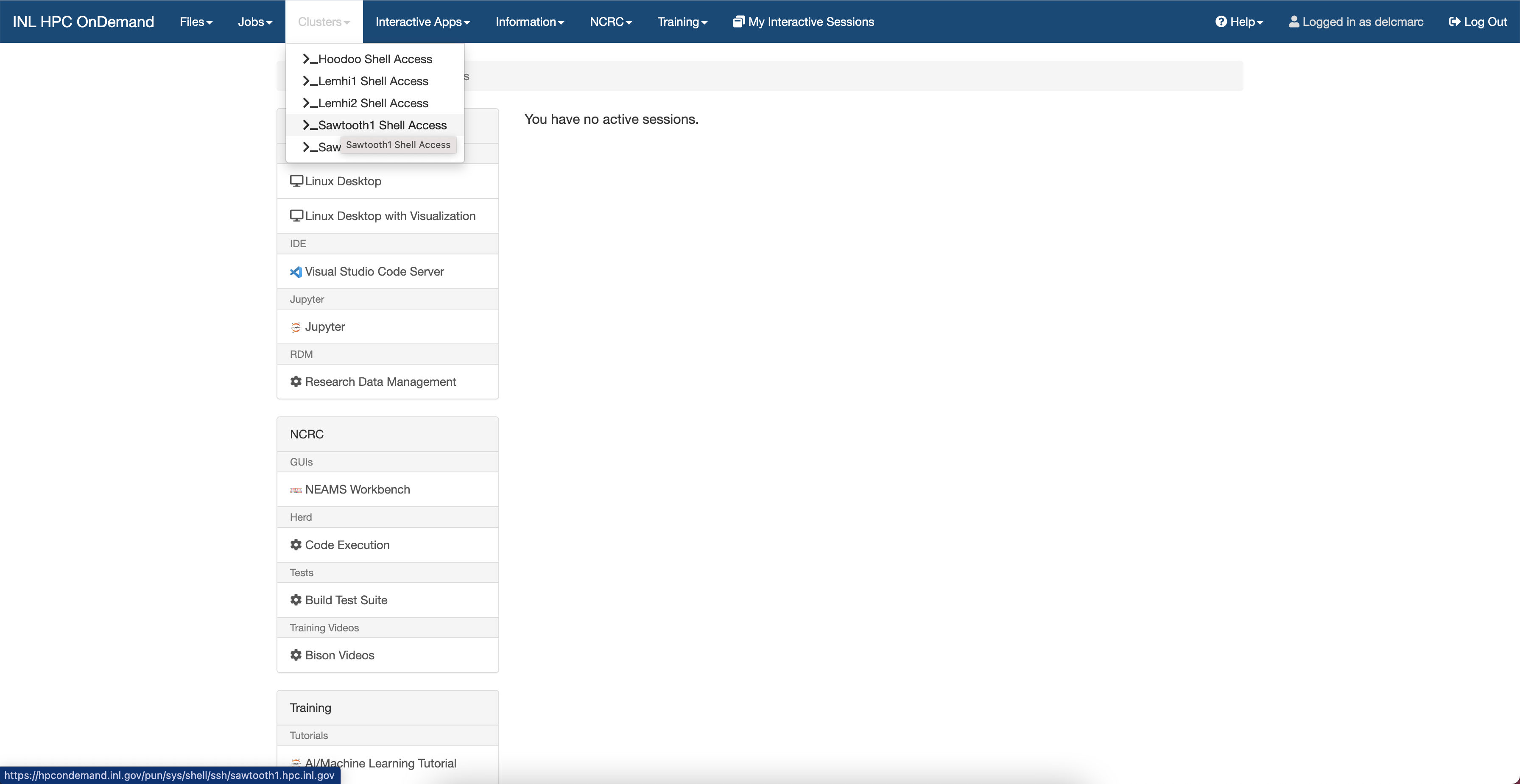
Figure 1: Accessing Sawtooth terminal on the INL HPC OnDemand website.

The Sawtooth terminal should immediately start as seen in Figure 2:

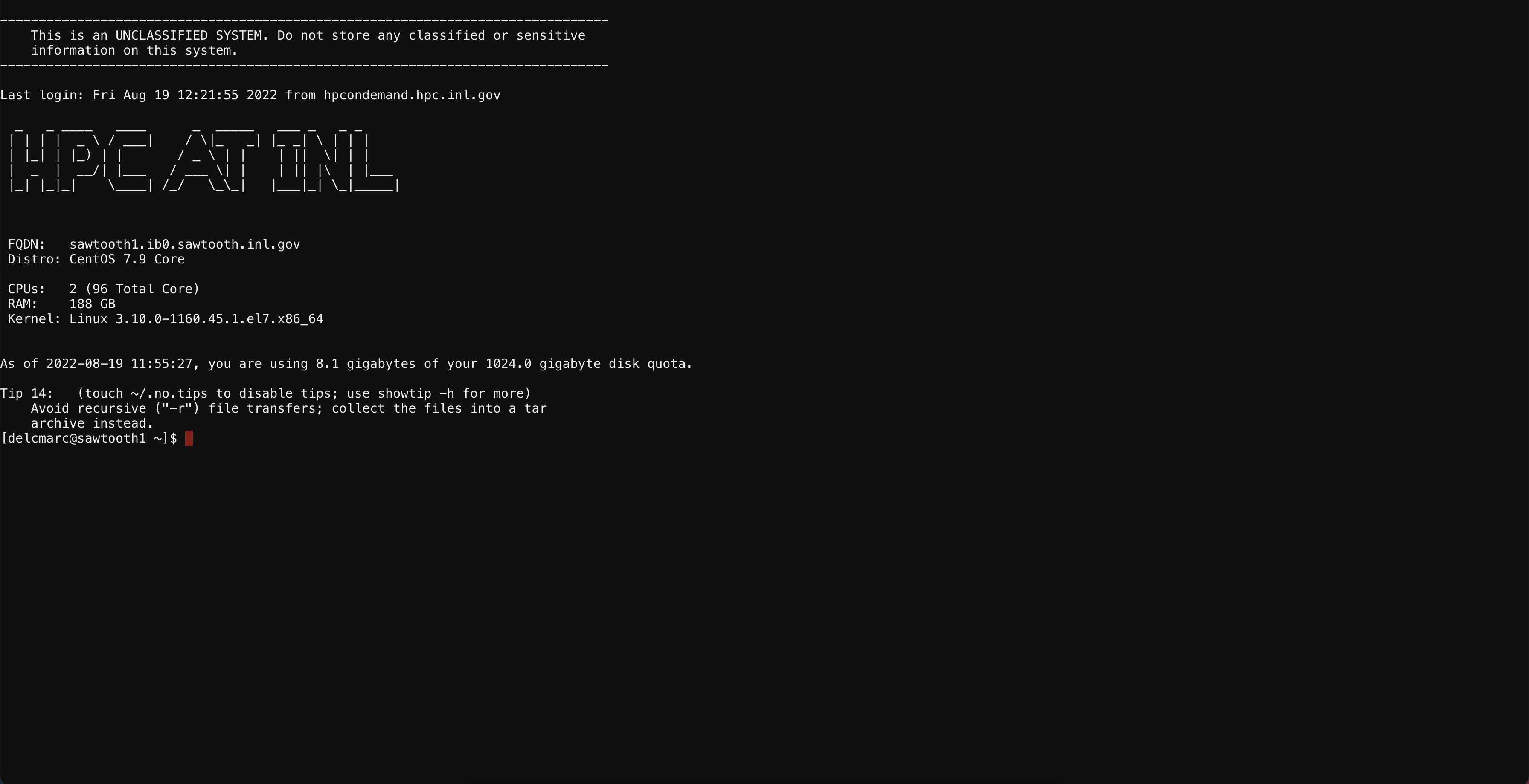
Figure 2: Sawtooth terminal on the INL HPC OnDemand website.

Once the terminal is opened, the VTB GitHub repository can be cloned. The first step is to load the gitlfs module and to install Git LFS locally. Git-LFS is needed to clone large size files (mesh, database, ...) present in the VTB GitHub repository:

module load gitlfs; git lfs install

If successful, the terminal should show Git LFS initialized. Once git-lfs is enabled, copy the successive command lines to your Sawtooth terminal and hit enter to clone the VTB repository:

git clone https://github.com/idaholab/virtual_test_bed.git virtual_test_bed

The output of the above command line is as follows:

Cloning into 'virtual_test_bed'...
remote: Enumerating objects: 4524, done.
remote: Counting objects: 100% (885/885), done.
remote: Compressing objects: 100% (366/366), done.
remote: Total 4524 (delta 534), reused 719 (delta 502), pack-reused 3639
Receiving objects: 100% (4524/4524), 112.31 MiB | 39.01 MiB/s, done.
Resolving deltas: 100% (2487/2487), done.
Downloading htgr/htr10/data/mesh/htr-10-critical-a-rev6.e (2.7 MB)
Downloading htgr/htr10/data/mesh/htr-10-full-a-rev3.e (3.5 MB)
Downloading htgr/htr10/data/sph/htr-10-Diff-SPH.xml (3.0 MB)
Downloading htgr/htr10/data/xs/htr-10-XS.xml (4.9 MB)
Downloading htgr/htr10/steady/gold/out-HTR-10-full-Diff-SPH-ARO.e (7.4 MB)
Downloading htgr/htr10/steady/gold/out_HTR-10_critical.e (7.9 MB)
Downloading htgr/pbmr400/shared/oecd_pbmr400_tabulated_xs.xml (212 MB)
Downloading mrad/mesh/mrad_mesh.e (62 MB)
Downloading pbfhr/reflector/conduction/conduction.fld (247 MB)
Downloading pbfhr/reflector/meshes/fluid.re2 (60 MB)
Downloading pbfhr/reflector/meshes/solid.e (62 MB)
Checking out files: 100% (370/370), done.

The content of the virtual_test_bed directory can be accessed with the ls command:

ls virtual_test_bed/
apps  COPYRIGHT  doc  htgr  LICENSE  mrad  msr  pbfhr  README.md  scripts  sfr

All VTB examples are run with the BlueCrab application.

Conventional Workflow on an HPC Platform

Conventionally, a modeling and simulation application is run on an HPC platform in a terminal by following four steps.

• Step 1: connect to the remote HPC platform using Secure Shell or one of its derivatives.

• Step 2: enter the working directory of choice, then edit the input file and any other relevant files, including the mesh files.

• Step 3: submit the job to the scheduler using a submission script from the working directory. The submission script contains logic to load the correct environment as well as the executable to run and the number of cores to use.

• Step 4: once the job is completed, visualize and analyze the numerical solution using a data visualization application, such as VisIt or ParaView. Data visualization may require copying large result files from the cluster to a desktop environment.

This workflow can be cumbersome to users unfamiliar with HPC platforms and an obstacle to potential industrial users in the nuclear engineering field who want to leverage HPC resources to speed up calculations. NCRC intends to increase the accessibility of modeling and simulation codes and the use of HPC resources by allowing users to access an HPC login node through a virtual desktop from the login page of the HPC OnDemand website (step 1). From there, users can run an application (BlueCrab) or open a terminal to edit files but still need their own submission script to submit jobs to the scheduler.

Bridging the Gap with the NEAMS Workbench

The NEAMS Workbench is now available on the HPC OnDemand website as a GUI under the NCRC tab and provides the means for performing steps 1–4. The following sections provide details on how to perform the above successive steps. All steps are also illustrated in a demonstration video.

Step 1: creating a NEAMS Workbench session on Sawtooth using the HPC OnDemand website

After connecting the HPC OnDemand website by entering the username and the passcode, the virtual Desktop opens as shown in Figure 3.

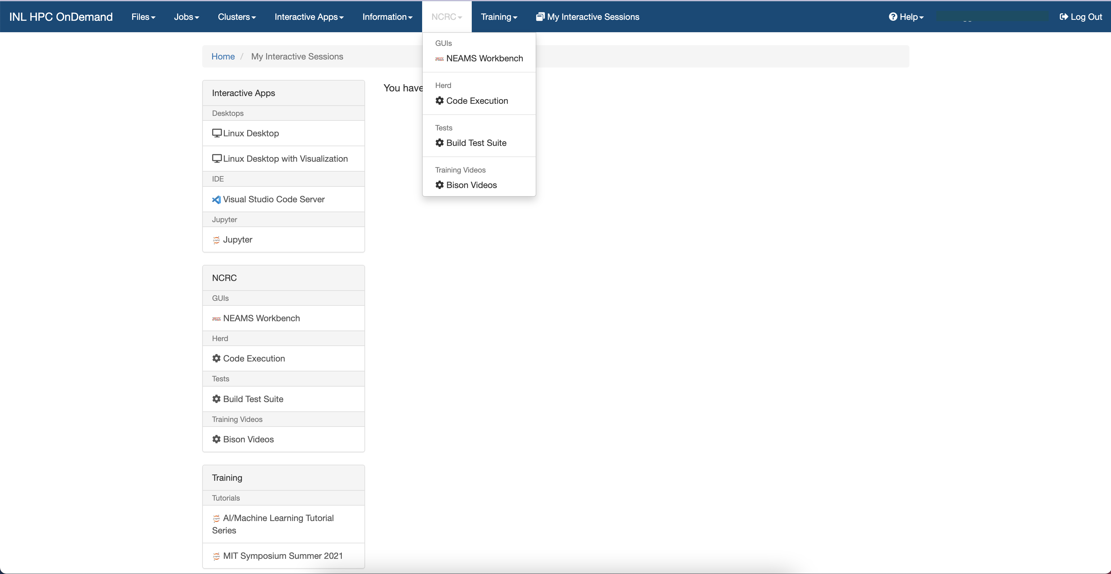
Figure 3: Accessing the NEAMS Workbench GUI on the INL HPC OnDemand website.

After clicking on NCRC, select NEAMS Workbench, enter Number of hours and Cores as shown in Figure 4, and then click on Launch to submit the request to the scheduler. Note that the session will run the NEAMS Workbench GUI and not an actual job. Consequently, selecting one to four cores is sufficient. By default, the session runs on four cores with a wall time of 1 hour, which can be edited upon selection.

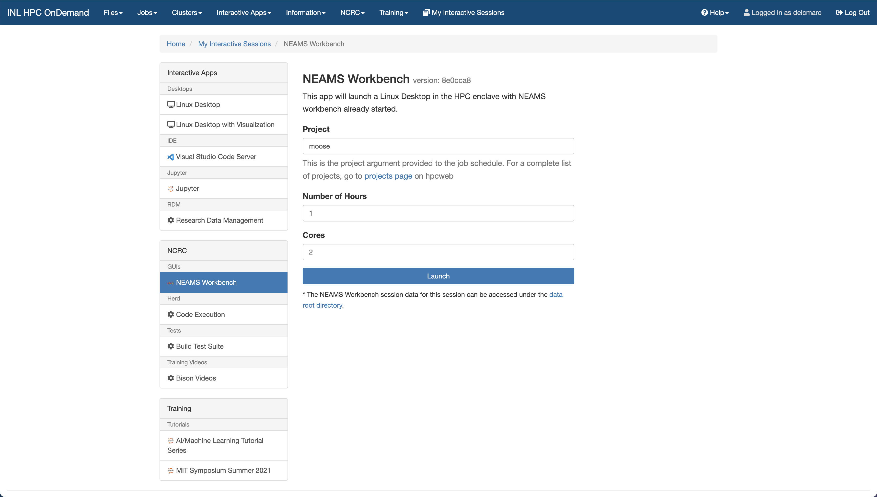
Figure 4: Create a NEAMS Workbench session on Sawtooth.

The session can take a few minutes to start (Figure 5).

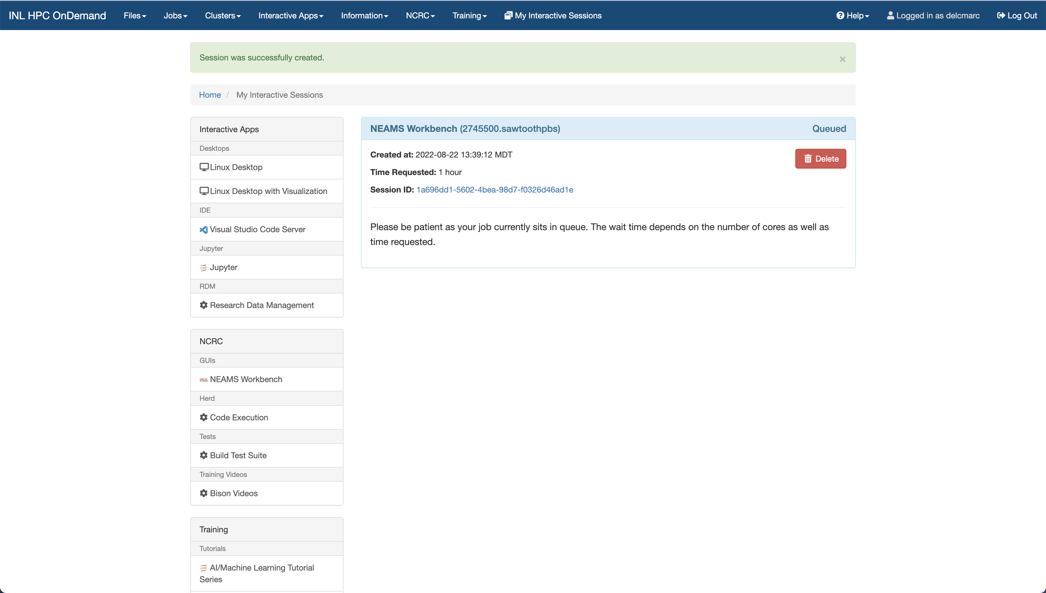
Figure 5: Waiting for a NEAMS Workbench session to start.

Once the session has started to run, the webpage is updated (Figure 6), and the NEAMS Workbench GUI can be launched by clicking on Launch NEAMS Workbench. A virtual Linux Desktop opens and automatically starts the NEAMS Workbench GUI as displayed in Figure 7.

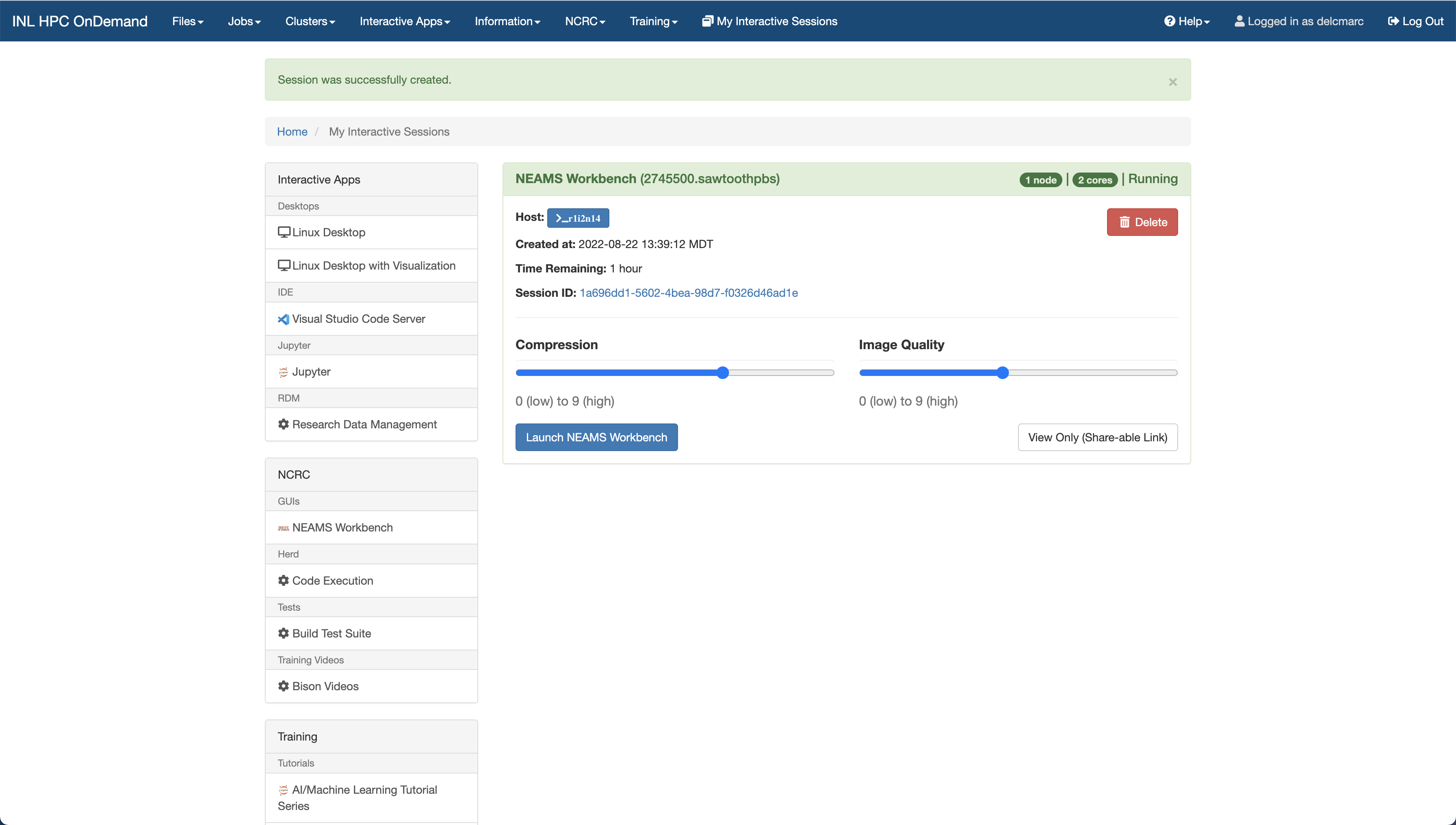
Figure 6: Launch NEAMS Workbench session on Sawtooth.

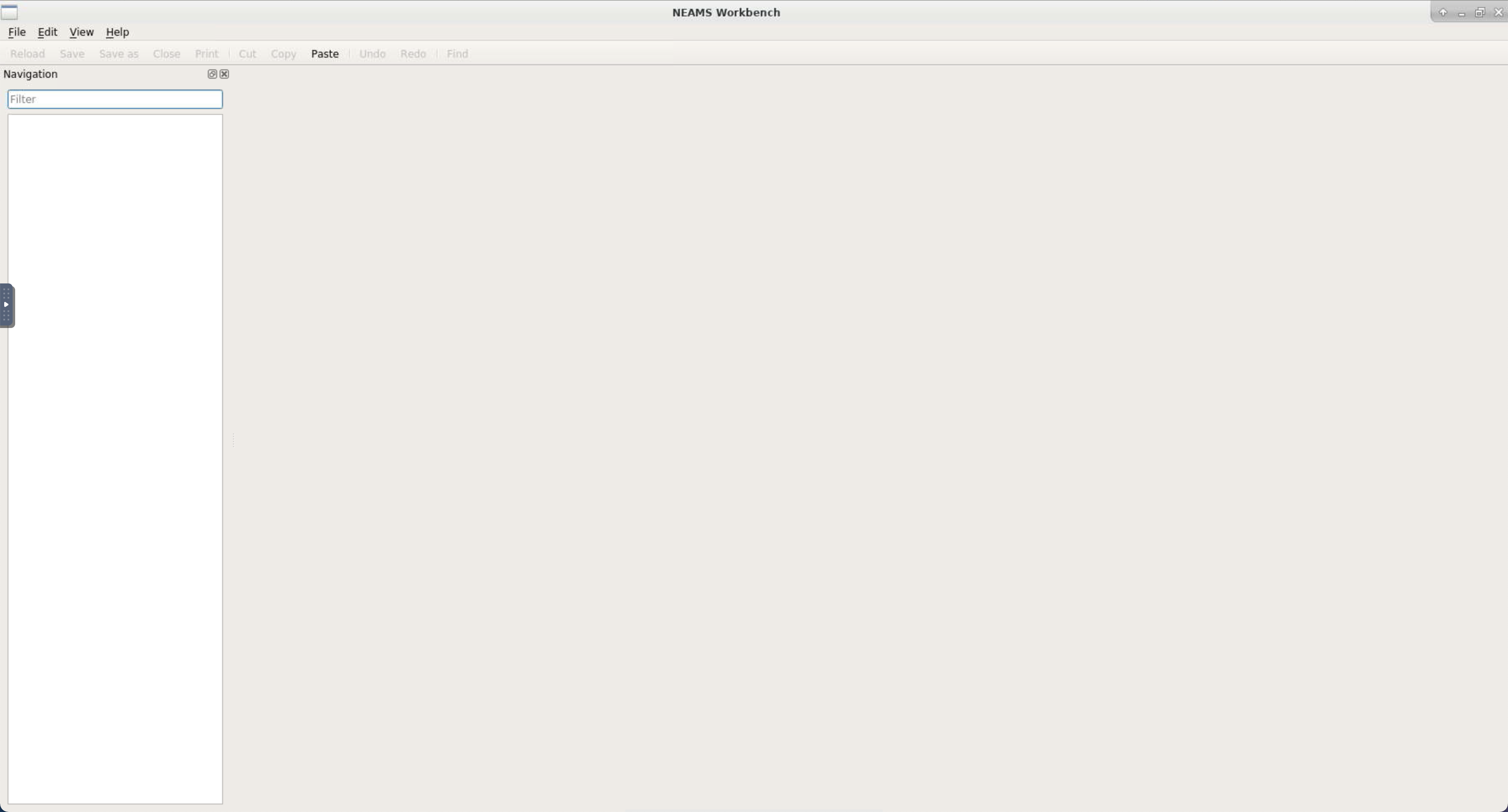
Figure 7: NEAMS Workbench GUI on Sawtooth.

Step 2: enabling the BlueCrab executable and uploading an input file to edit

Once the NEAMS Workbench GUI (see step 1) has been initialized, the user should set the environment for the Blue-Crab application, which consists of loading modules and making the executable available in the path. This is achieved through the NEAMS Workbench GUI by clicking File and Localhost. A widget opens and lists all Moose applications available on Sawtooth. The widget should be enlarged with the mouse cursor. The Blue Crab application or any other MOOSE-based applications to activate is selected by (1) clicking on the number to the left of the application name and (2) Activate. The output of the process is shown in the tab below the list of all MOOSE-based application and is deemed successful once the content {"Completed" : true} is displayed as illustrated in Figure 8. Note that activation process sets up the correct Linux environment for the MOOSE-based application and also loads various files needed by the NEAMS Workbench GUI for auto-completion and validations of the input files.

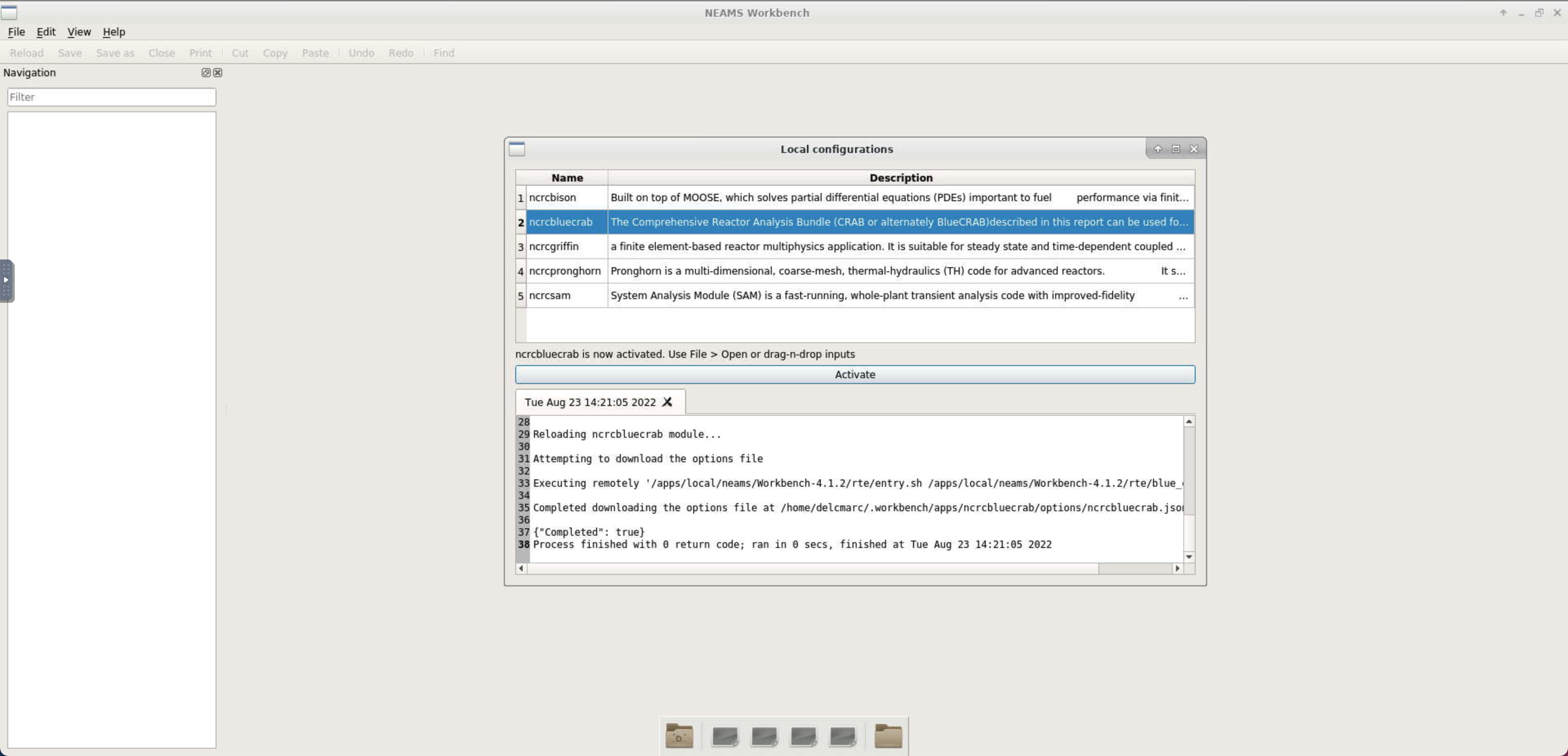
Figure 8: Enabling the BlueCrab environment from the NEAMS Workbench GUI.

The next step consists of opening an input file from the NEAMS Workbench GUI, which is demonstrated with the sodium-cooled fast reactor example (SFR) from the VTB website. Assuming that the VTB repository files were already cloned to the INL HPC filesystem (see here), several input files are available and can be navigated to within Workbench. Users can load the griffin.i input files (main application or main app) for the SFR VTB example by clicking File and then Open File. A window should open and allow the user to navigate through the content of the home directory. Click on virtual_test_bed and then sfr to access the input files (Figure 9).

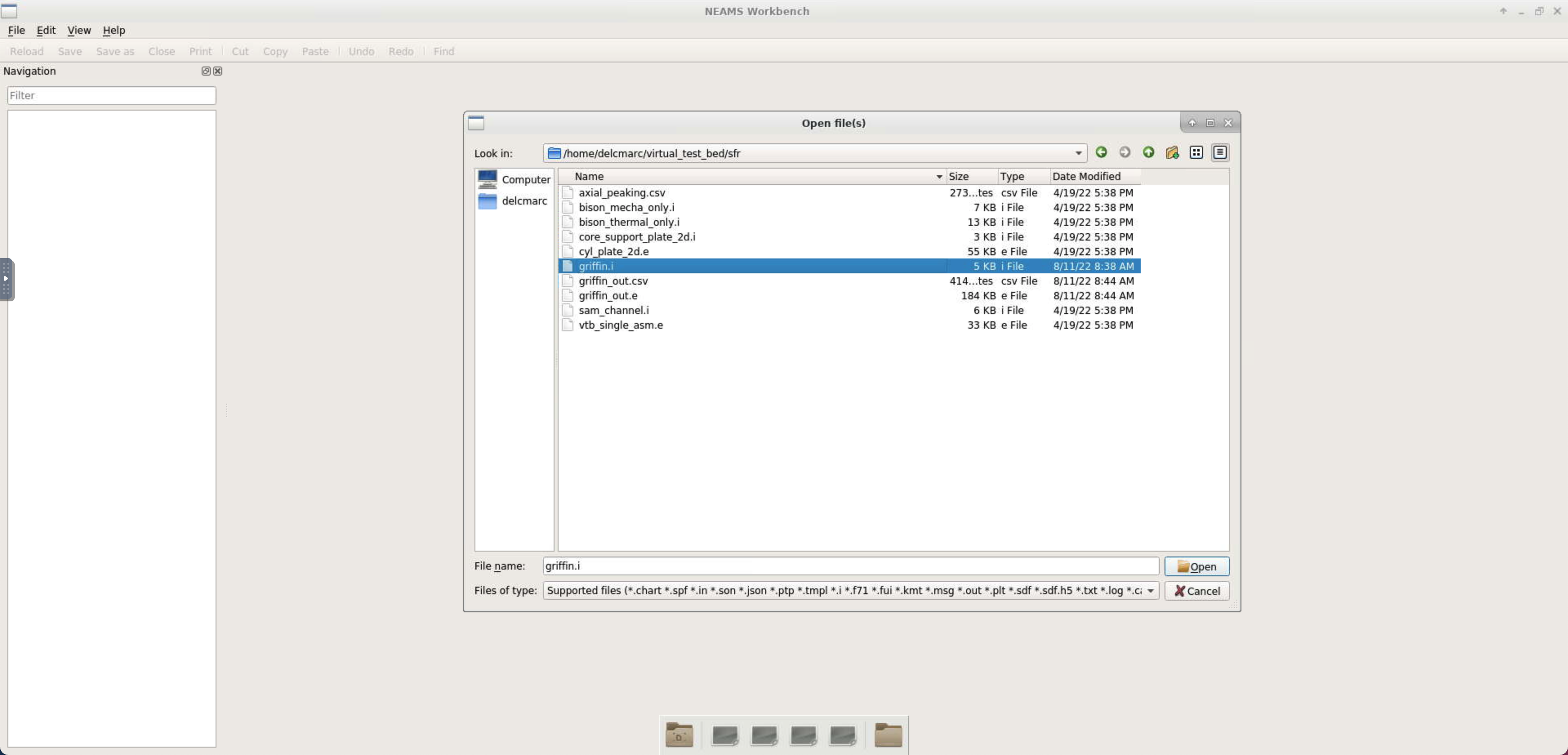
Figure 9: Open griffin.i input file with the NEAMS Workbench.

After opening the input file, the Navigation tab shows all input file blocks, sub-blocks, and their content to ease navigation in the input file. Each block can be extended to show its content. Make sure the NEAMS Workbench automatically updates the correct schema and runtime environment to ncrcbluecrab - ncrcbluecrab (left and right of the dropdown box named document). The Exodus mesh file vtb_single_assembly_asm.e is also opened within the NEAMS Workbench by following the same steps as those for the main app input file. Once opened and after splitting screen (click on the tab name srf:vtb_single_asme.e and drag and drop in the right-hand side of the GUI), users can highlight specific mesh blocks from the input file by right-clicking on the mesh block name and selecting Inspect, as shown for mesh block 2 (line 67) in Figure 10. Users can also easily identify geometry components to assign material properties, kernels, initial conditions, or boundary conditions. The same capabilities are also available for all sub-application (sub-app) input files.

Validation of the input file is automatically handled by the NEAMS Workbench GUI, and validation errors are shown in the Validation tab highlighted in red and located at the bottom right of the GUI, see Figure 10. It should be noted that some of the validation errors are due to some syntax not being supported by the NEAMS Workbench. These issues are being addressed and will be fixed in a future release of the NEAMS Workbench GUI. These particular validation errors can be ignored for now and will not prevent the job from running properly (see this section for further details). By clicking on the validation error message, the user is taken to the line with the syntax error. Auto-completion is also available to help with file editing, which is illustrated at time 1:41 in the demonstration video.

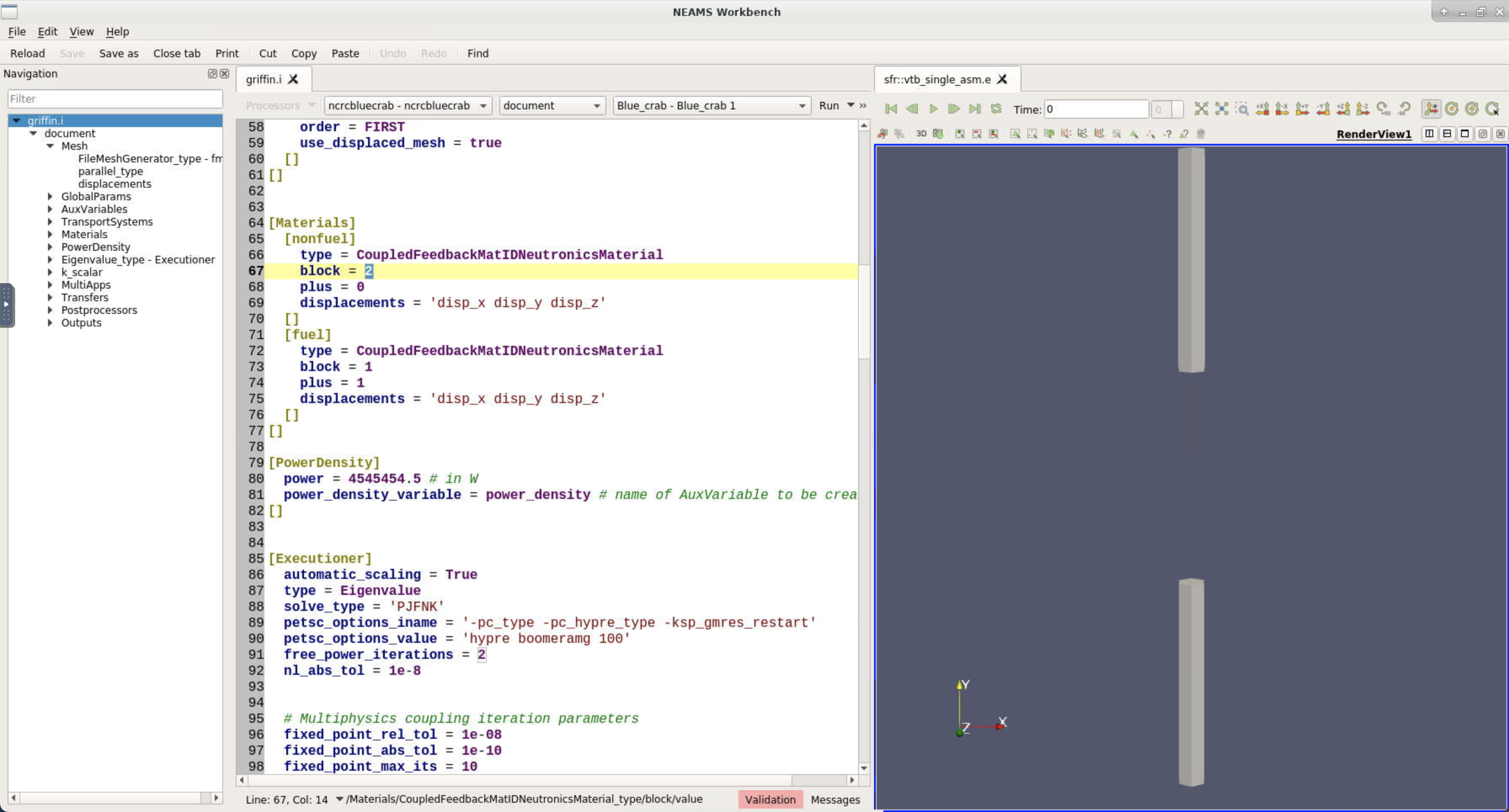
Figure 10: Input file (left) and mesh visualization (right) with the NEAMS Workbench.

Step 3: running a job from the NEAMS Workbench GUI

After editing the input file and making sure that the physics enabled are consistent with the geometry visualized with ParaView, the input file is submitted to the scheduler. The NEAMS Workbench has already been set to run this input file with the _BlueCRAB_ executable (configured in Step 1). To submit the job to Sawtooth, simply type Run, which will create the required job scheduler script behind the scenes and put your job in the queue. To customize your job run options first, click the downward arrow next to Run and select Customize Run Options.... A widget opens that allows users to modify the number of cores and CPU time by scrolling down to Remote: Scheduler Header and modifying the number of nodes (select), numbers of CPUs per node (ncpus) and wall time (wall time), as illustrated in Figure 11. The suggested number of nodes/CPUs and wall time should be given in the VTB documentation for each test case. Progress of the job is displayed in the Message: the NEAMS Workbench checks on the status of the job and tail the output once it starts to run on Sawtooth. Once the job completes, it will display Process Finished.

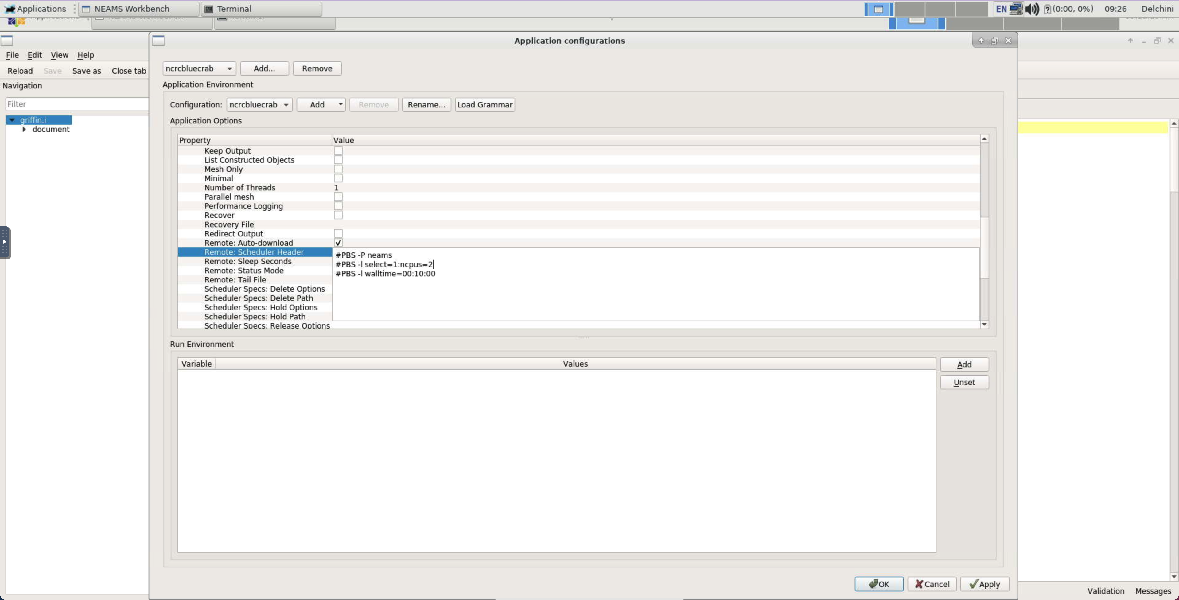
Figure 11: Editing PBS options with the NEAMS Workbench GUI.

Step 4: visualize the numerical solution from the NEAMS Workbench GUI

Visualization of the numerical solution is also achieved within the NEAMS Workbench GUI. Users can refer to the steps below or watch the demonstration video starting at 4:20. As for visualizing the geometry and the mesh described in Step 1, the Exodus file that contains the numerical solution can be visualized with the built-in ParaView, as shown in Figure 16. The same steps as in 4.2.1 can be followed. An alternative way is to right click on the name of the input file in the Navigation tab and select Open working directory. From there, a navigation window opens with all files contained in the working directory. The Exodus file griffin_out.e can be dragged and dropped in the NEAMS Workbench GUI. A visualization tab or render view should automatically open and display the geometry as shown in Figure 12.

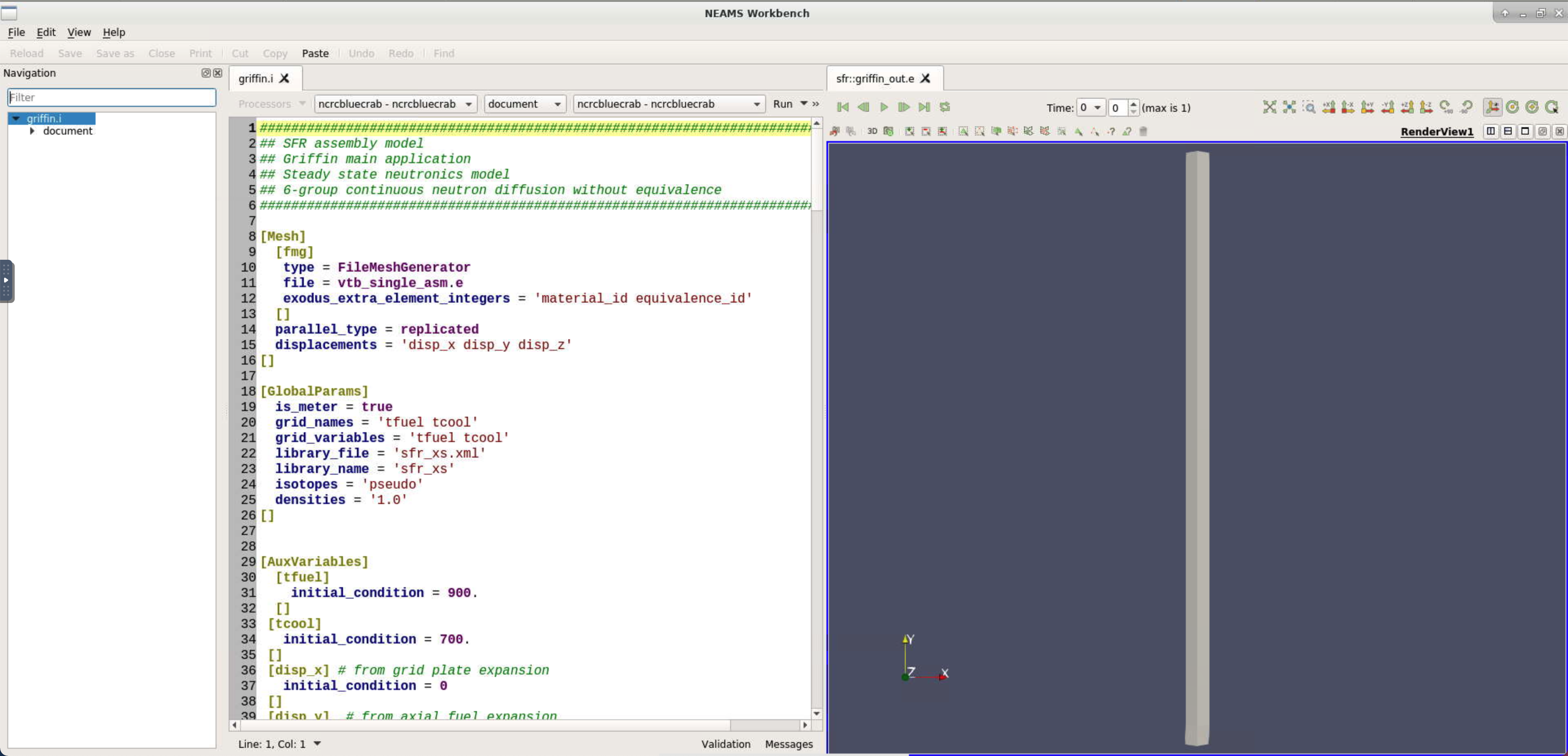
Figure 12: Drag and drop the Exodus solution output file griffin_out.e in the NEAMS Workbench GUI to open a visualization tab or render view.

The ParaView GUI is enabled by clicking on Visualization and checking the box for Visualization GUI. The Visualization GUI appears in the right-hand side of the NEAMS Workbench GUI with ParaView options as seen in Figure 13. After enabling all variables and clicking Apply within the Visualization GUI, a variable can be plotted by right-clicking on the geometry in the visualization tab and selecting Color by and then the name of the variable of interest ( Figure 14 and Figure 15 ). The Visualization tab can also be split to plot multiple variables side-by-side, as seen in Figure 16.

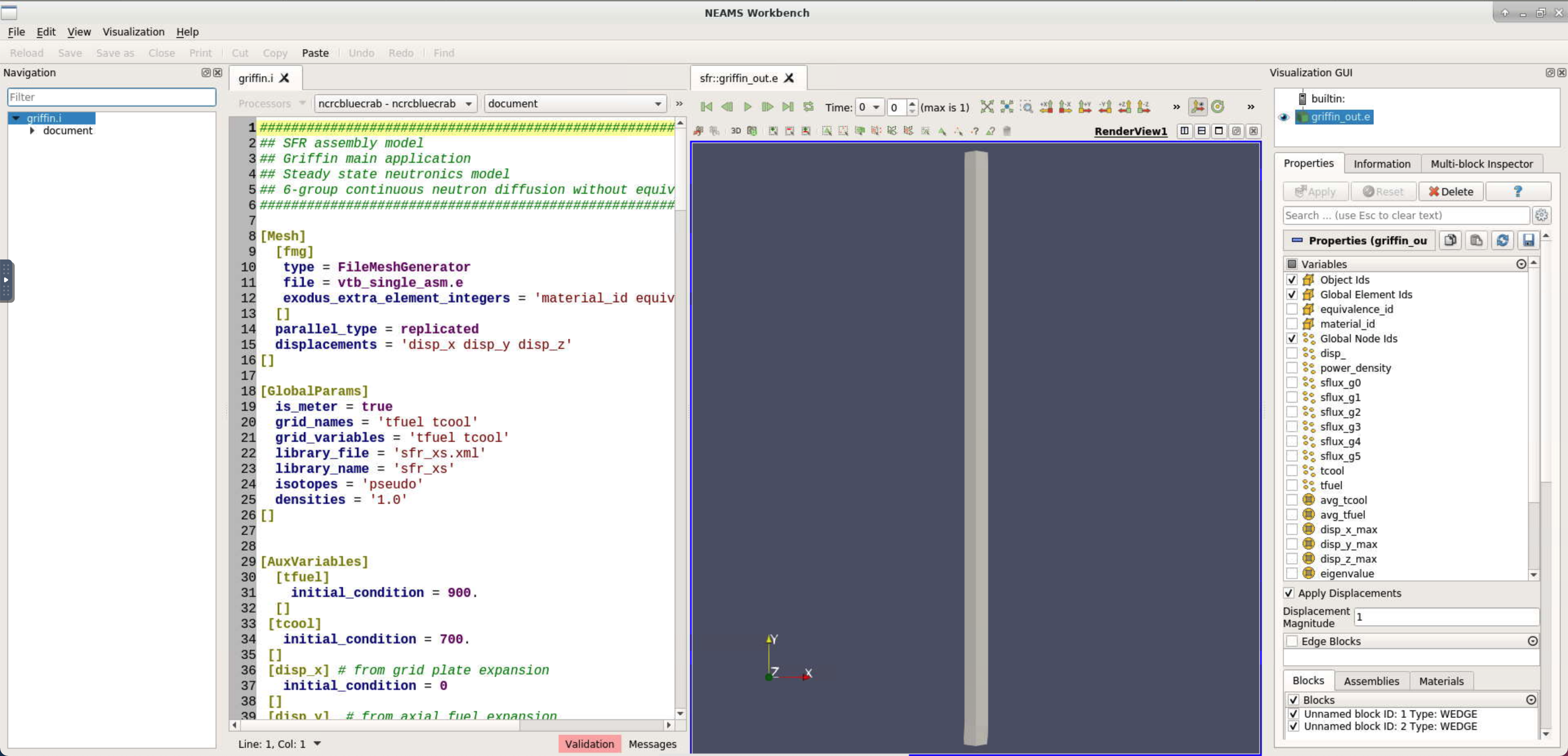
Figure 13: Enabling the Visualization GUI for ParaView.

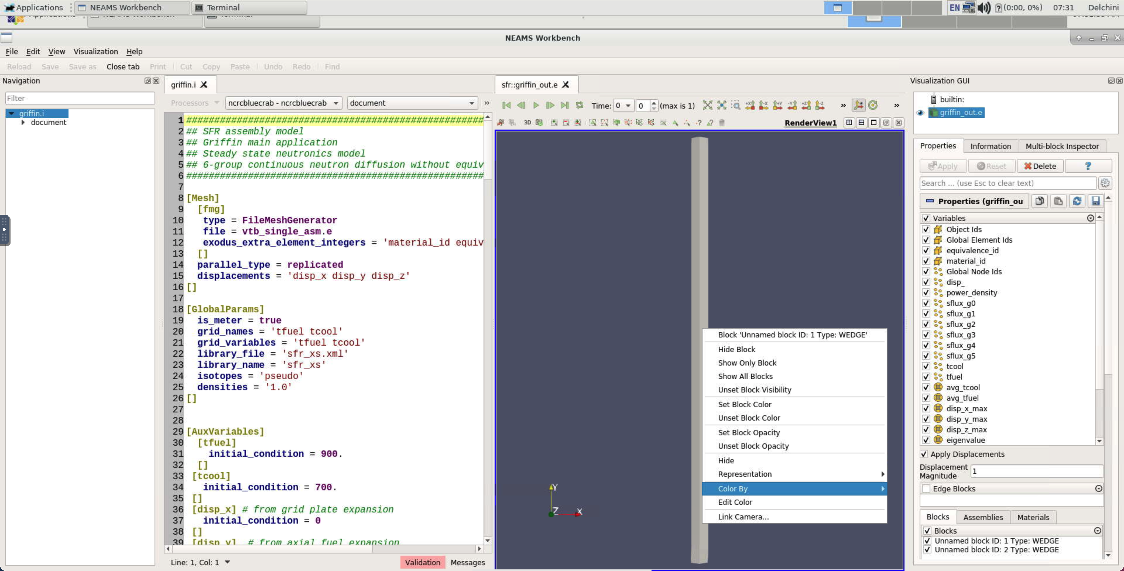
Figure 14: After right-clicking on the geometry in the Visualization tab, select Color by to access all variables to plot.

Figure 15: NEAMS Workbench GUI showing power density profile in the Visualization tab.

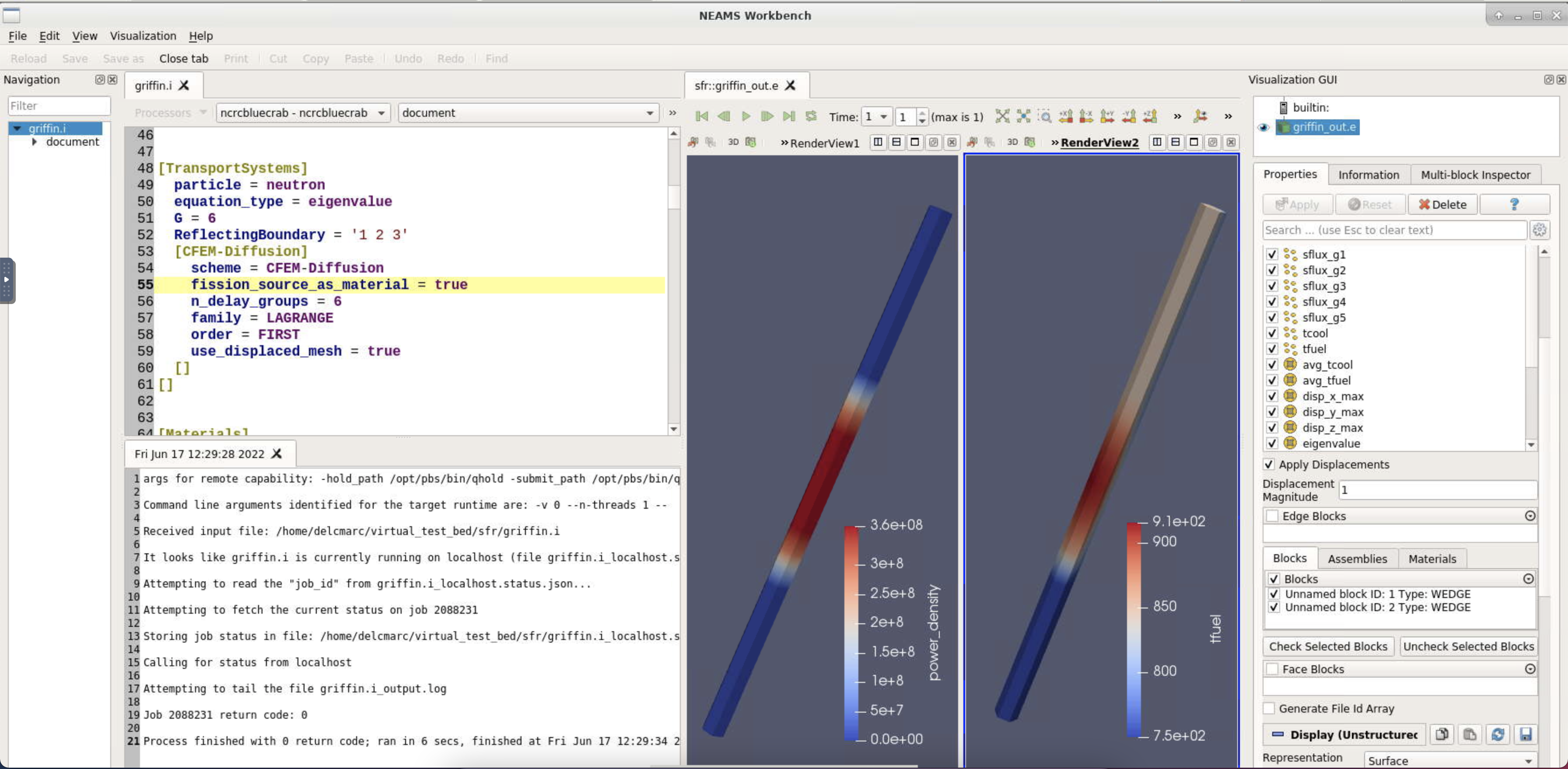
Figure 16: The NEAMS Workbench GUI with griffin.i input file (top left), the output from the scheduler (bottom left), and the numerical solution visualized with ParaView (right).

Exiting and closing the Virtual Desktop

The Virtual Desktop can be exited by closing the browser tab that was opened when creating a NEAMS Workbench session in Step 1. Users have the option of logging back in by clicking Launch the NEAMS Workbench shown in Figure 6. The NEAMS Workbench session can be closed by clicking on Delete, which will terminate the session.