1. Introduction to Multiphysics Coupling with MOOSE
Analysis of nuclear reactor systems often requires multiphysics modeling, e.g. the modeling of multiple sets of governing partial differential equations (PDEs) that solves different "physics" of the system, including
radiation transport
fluid dynamics
heat conduction
structural mechanics
fuel behavior
chemistry
systems behavior
A physics model is "coupled" to another physics model if it has dependencies on variables computed by another system of equations. For example, the neutron transport equation utilizes material cross sections which depend on temperature, but temperature is calculated by other governing equations which require the power distribution from the neutron transport equation. The coupling from one physics to another may be important in some reactor systems and negligible in others.
Several approaches are available to numerically solve coupled physics problems: full, tight, and loose coupling. The MOOSE framework was originally designed to solve coupled PDEs using the fully coupled approach, but tight or loose coupling approaches are also available using the MultiApp System. The MultiApp approach is commonly used for multiphysics reactor analysis, as seen by many examples hosted on this website. Before discussing MultiApps in more detail, we first describe the three coupling approaches and when they are appropriate.
Fully, Tightly, and Loosely Coupled Systems
To illustrate the differences between full, tight, and loose coupling, we introduce a simple example. Eq. (1) consists of two coupled equations for two variables (solution vectors), and (e.g., displacement and temperature in a thermal stress problem).
(1)
If and are both zero matrices, and are independent from each other and no coupling is needed - each equation can be solved independently without consideration to the other equation. Otherwise, the variables can be computed by assembling the two equations into a single matrix system as shown in Eq. (2). Direct solution of Eq. (2) is known as full coupling (see Figure 1).
(2)
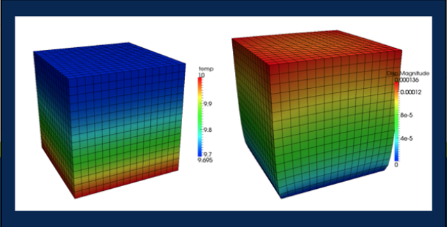
Figure 1: Schematic of a pair of systems solved by full coupling, as represented by the box around both systems (courtesy of Derek Gaston).
Alternatively, the solutions satisfying Eq. (1) can be determined through tight or loose coupling schemes, in which each set of equations is solved separately for one variable while holding the other variable fixed. Eq. (2) can be rewritten as:
(3)
Eq. (3) can then be numerically solved by an iterative approach called Picard iteration illustrated in Eq. (4).
(4)
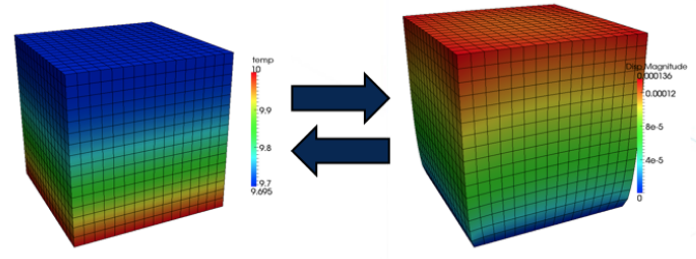
Figure 2: Schematic of a pair of systems solved by tight coupling, as indicated by arrows going both ways between the individual system solves representing information transfer during one time step (courtesy of Derek Gaston).
As shown in Eq. (4), each equation within Eq. (1) is solved individually for only one variable while holding the other variable constant (based on its previous iteration value or initial guess). After each system solve, updated values for the computed variable are provided to the other system, which holds the non-computed variable constant during its solve. If the iterations are repeated for a given timestep until the solutions satisfy a global convergence criteria, the coupling approach is said to be tight (see Figure 2). If only one iteration is performed for a given timestep without consideration of convergence, the coupling is said to be loose (see Figure 3).
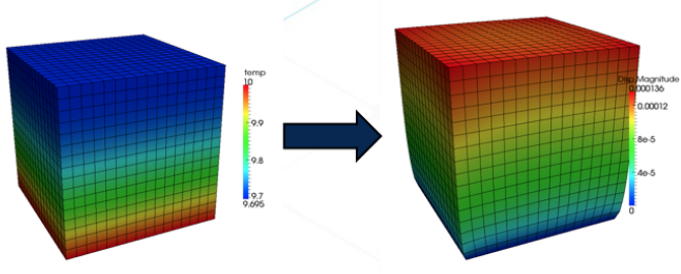
Figure 3: Schematic of a pair of systems solved by loose coupling, as indicated by the single arrow representing information transfer during one timestep. Note that information from the second system can be transferred back to the first system at the beginning of the next timestep. (courtesy of Derek Gaston).
In MOOSE, a fully coupled solve is invoked by adding related PDE terms into a single MOOSE input file Kernels block, whereas the tightly and loosely coupled solution approaches are established through its MultiApp system. MultiApp input blocks may be defined in different application input files to allow the user to simultaneously solve for individual physics systems and to control the communication frequency and type of communicated information between codes. The MultiApp system can be used to connect MOOSE-based and MOOSE-wrapped applications in customized, flexible coupling schemes.
In addition to being used to solve multiphysics problem, the MultiApp system is also capable of handling uncertainty assessment or sensitivity analysis through the MOOSE Stochastic Tools module.
When to Use the MultiApp Coupling Approach
MOOSE was created to solve fully-coupled systems of PDEs with efficient convergence. However, tight or even loose coupling using MultiApps is a better approach in many reactor analysis situations. When the systems of equations involve disparate time scales or space scales, or when the coupling is weak in one direction, full coupling will be computationally burdensome and a tight/loose coupling approach using MultiApps is advised.
Disparate Time Scales
Many coupled physical phenomena involve disparate time scales (one variable changes slowly over time and requires large time steps to capture its transient behavior, while another variable changes rapidly and requires small time steps). Using a fully coupled system to solve coupled phenomena with disparate time scales would waste considerable computational resource because it forces the slowly-evolving variable to use a small time step. Using a tightly or loosely coupled system enabled by the MultiApp system allows the two variables to be solved on different time steps.
Disparate Space Scales
Coupled physical phenomena may involve vastly different space scales (one variable is related to macroscopic phenomenon, while another variable involves localized or microstructure details). Using a fully coupled system on problems with disparate space scales would waste considerable computational resource on solving the macroscopic variables on an unnecessarily fine mesh to accommodate the other variable's meshing needs. The MultiApp system permits the different variables to be solved separately, using their own meshes. In some cases, the meshes may even have different dimensions (1D vs 2D vs 3D).
Weak Coupling or Uni-Directional Coupling
When one physics does not make a large impact on another physics solution, we say the two phenomena are weakly coupled. For example, in reactor designs with small thermal reactivity coefficients, small changes in coolant temperature will cause very small changes in reactivity and power. However, changes in power may still lead to dramatic changes in coolant and fuel temperatures. The MultiApp approach provides a flexible way to solve each physics as often as needed (including potentially only once).