Bypass Flow Reflector Modeling
Contact: April Novak, anovak.at.anl.gov
Model link: FHR Bypass Flow Reflector Model
The meshes for this model are hosted on LFS. Please refer to LFS instructions to download them.
The pebble region in the Pebble Bed Fluoride-Salt-Cooled High-Temperature Reactor (PB-FHR) is enclosed by an outer graphite reflector that constrains the pebble geometry while also serving as a reflector for neutrons and a shield for the reactor barrel and core externals. In order to keep the graphite reflector within allowable design temperatures, the reflector contains several bypass flow paths so that a small percentage of the coolant flow, usually on the order of 5 to 10% of the total flow, can remove heat from the reflector and maintain the graphite within allowable temperature ranges. This bypass flow, so-named because coolant is diverted from the pebble region, is important to quantify during the reactor design process so that accurate estimates of core cooling and reflector temperatures can be obtained.
This page shows an example of using nekRS, a Graphics Processing Unit (GPU) based Computational Fluid Dynamics (CFD) code developed by Argonne National Laboratory, coupled to MOOSE to explore the conjugate heat transfer in a small region of the PB-FHR reflector. With input from a full-core coupled Pronghorn-Griffin model, this example can be used to evaluate hot spots in the reflector and ensure that temperatures remain within allowable limits. The meshes for this example are created with programmable scripts; by running these mesh scripts for a range of bypass gap widths and repeating the flow simulations for a range of Reynolds numbers, this model can be used to provide friction factor and Nusselt number correlations as inputs to a full-core Pronghorn model.
The objectives of the present analysis are to:
Show an example of how non-MOOSE codes can be coupled to MOOSE, and some capabilities in this space for thermal-hydraulics analysis. You should come away with an understanding of what a "MOOSE-wrapped app" looks like and the extent to which MOOSE-wrapped applications behave like other natively-developed MOOSE applications.
Predict the pressure, velocity, and temperature distribution in the PB-FHR outer reflector.
Describe how high-resolution tools such as nekRS can be used to generate closure terms (such as friction factor models) for the coarse-mesh tools in the MOOSE framework, such as Pronghorn.
nekRS uses the Open Concurrent Compute Abstraction (OCCA) Application Programming Interface (API), which allows nekRS to run on both Central Processing Unit (CPU) and GPU systems. However, in this example, nekRS is used with resolved boundary layers, requiring a fine mesh. This analysis therefore requires High-Performance Computing (HPC) resources. If you do not have access to HPC resources, you will still find the analysis procedure useful in understanding the MOOSE-wrapped app concept and opportunities for high-resolution thermal-hydraulics within the MOOSE framework.
Cardinal and MOOSE-Wrapped Apps
The analysis shown here is performed with Cardinal, a MOOSE application that "wraps" nekRS, a CFD code, and OpenMC, a Monte Carlo particle transport code. Cardinal is an open-source application, available on GitHub. As this example focuses on heat transfer modeling, there will be no further discussion of the OpenMC wrapping in Cardinal. "Wrapping" means that, for all intents and purposes, nekRS simulations can be run within the MOOSE framework and interacted with as if the physics and numerical solution performed by nekRS were a native MOOSE application. Cardinal contains source code that facilitates data transfers in and out of nekRS and runs nekRS within a MOOSE-controlled simulation. At a high level, Cardinal's wrapping of nekRS consists of:
Constructing a "mirror" of the nekRS mesh through which data transfers occur with MOOSE. For conjugate heat transfer applications such as those shown here, a MooseMesh is created by copying the nekRS surface mesh into a format that all native MOOSE applications can understand.
Adding MooseVariables to represent the nekRS solution. In other words, if nekRS stores the temperature internally as an
std::vector<double>, with each entry corresponding to a nekRS node, then a MooseVariable is created that represents the same data, but that can be accessed in relation to the MooseMesh mirror.Writing multiphysics feedback fields in/out of nekRS's internal solution and boundary condition arrays. So, if nekRS represents a heat flux boundary condition internally as an
std::vector<double>, this involves reading from a MooseVariable representing heat flux (which can be transferred with any of MOOSE's transfers to the nekRS wrapping) and writing into nekRS's internal vectors.
Accomplishing the above three tasks requires an intimate knowledge of how nekRS stores its solution fields and mesh. But once the wrapping is constructed, nekRS can then communicate with any other MOOSE application via the MultiApp and Transfer systems in MOOSE, enabling complex multiscale thermal-hydraulic analysis and multiphysics feedback. The same wrapping can be used for conjugate heat transfer analysis with any MOOSE application that can compute a heat flux; that is, because a MOOSE-wrapped version of nekRS interacts with the MOOSE framework in a similar manner as natively-developed MOOSE applications, the agnostic formulations of the MultiApps and Transfers can be used to equally extract heat flux from Pronghorn, BISON, the MOOSE heat conduction module, and so on.
Cardinal allows nekRS and OpenMC to couple seamlessly with the MOOSE framework, enabling in-memory coupling, distributed parallel meshes for very large-scale applications, and straightforward multiphysics problem setup. Cardinal has capabilities for conjugate heat transfer coupling of nekRS and MOOSE, concurrent conjugate heat transfer and volumetric heat source coupling of nekRS and MOOSE, and volumetric density, temperature, and heat source coupling of OpenMC to MOOSE. Together, the OpenMC and nekRS wrappings augment MOOSE by expanding the framework to include high-resolution spectral element CFD and Monte Carlo particle transport. For conjugate heat transfer applications in particular, the libMesh-based interpolations of fields between meshes enables fluid-solid heat transfer simulations on meshes that are not necessarily continuous on phase interfaces, allowing mesh resolution to be specified based on the underlying physics, rather than rigid continuity restrictions in single-application heat transfer codes.
The remainder of this page will describe the conjugate heat transfer capabilities of Cardinal.
Geometry and Computational Model
This section describes the PB-FHR reflector geometry and the simplifications made in constructing a computational model of this system.
This computational model is a simplified version of the actual reflector geometry and reactor state. Due to limitations in nekRS's boundary conditions, some geometry approximations will be made. This model is also run independently of Pronghorn and Griffin, so several assumptions are made regarding fluid boundary conditions at the inlet to the reflector and along the reflector-pebble bed interface, even though in reality the flow and heat transfer in the reflector is tightly coupled to the flow and heat transfer in the bed and the neutron transport over the entire reactor. It is important to be aware of these simplifications when assessing the physical predictions of this model. Nevertheless, these simplifications do not detract from the ability to use this model to learn about high-resolution conjugate heat transfer capabilities in the MOOSE framework as long as the simplifications are acknowledged. The details of this model can be refined for follow-on studies as needed.
A top-down view of the PB-FHR reactor vessel is shown below. This geometry is based on the specifications given in Shaver et al. (2019). The center region is the pebble bed core, which has an outer radius of 2.6 m. Surrounding the pebble region are two rings of graphite reflector blocks, staggered with respect to one another in a brick-like fashion. Each ring contains 24 blocks. The inner ring blocks have a width (i.e. radial thickness) of 0.3 m, while the outer ring blocks have a width of 0.4 m. The gaps between the blocks are 0.002 m wide. In black is shown the core barrel, which is 0.022 m thick. The gap between the outer ring of blocks and the barrel is ten times larger than the gap between the inner and outer ring of blocks, or 0.02 m.
 reactor core (only roughly to scale).](../../media/pbfhr/reflector/top_down.png)
Figure 1: Top-down schematic of the PB-FHR reactor core (only roughly to scale).
To ease the difficulty of meshing very narrow slots, as well as to make visualization and model depiction easier, the width of the gap between blocks is increased in this example to 0.006 m. Of course, over the lifetime of the reactor, the gap width changes due to graphite material response to fluence such that the gap width is not a fixed value. Therefore, we take this liberty here to improve visualization of the thin gaps, but allow setting the gap width as an input to the meshing scripts. Gap widths of 0.006 m are not completely without physical basis; for instance, for the Thorium High Temperature Reactor (THTR), a maximum 1% shrinkage of the graphite reflector blocks was assumed Oehme and Schöning (1970). Translating this percentage to the PB-FHR geometry corresponds to gaps of approximately 0.005 m thickness Novak et al. (2021).
To form the entire axial height of the reflector, rings of blocks are stacked vertically; each block is 0.52 m tall. The entire core height is 5.3175 m, or about 10 vertical rings of blocks (additional structures at the core inlet and outlet compose any remaining height not evenly divisible by 0.52 m).
In both the pebble bed region and through the small gaps between the reflector blocks and between the reflector blocks and the barrel, FLiBe coolant flows. This bypass flow path is shown as yellow dashed lines in Figure 1; in these gaps, coolant flows both from the pebble bed and outward in the radial direction, as well as vertically from lower reflector rings. Each ring of blocks is separated from the rings above and below it by very thin horizontal gaps that form as the graphite thermally expands (not shown in Figure 1; these flow paths also contribute to bypass flows, allowing a second radial flow path from the pebble bed towards the barrel. For simplicity, this second radial flow path is neglected here.
The total power of the PB-FHR is 236 MW; any power deposition in the reflector is neglected. The FLiBe inlet temperature to the core is 600°C, while the nominal outlet temperature is 700°C.
To reduce computational cost, the coupled nekRS-MOOSE simulation is conducted for a single ring of reflector blocks (i.e. a height of 0.52 m), with azimuthal symmetry assumed to further reduce the domain to half of an inner ring block, half of an outer ring block, and the vertical and radial bypass flow paths between the blocks and the barrel. This computational domain is shown outlined with a red dotted line in the figure above. As already mentioned, the second radial flow path (along fluid "sheets" between vertically stacked rings of blocks) is not considered. This geometry, as well as the boundary conditions imposed, will be described in much greater detail later when the meshes for the fluid and solid phases are discussed.
Governing Equations
This section describes the physics solved in this coupled conjugate heat transfer problem. Because there are no transient source terms or transient boundary conditions, the MOOSE heat conduction module will solve the steady state energy conservation equation for a solid,
(1)
where is the solid thermal conductivity, is the solid temperature, and is the solid volumetric heat source, which for this application is zero. Solving the steady energy conservation in lieu of the transient equation will accelerate the approach to the coupled pseudo-steady state.
nekRS solves the incompressible Navier-Stokes equations,
(2)
(3)
(4)
where is the fluid velocity, is the fluid density, is the pressure, is the viscous stress tensor, is a source vector, is a volumetric heat source, is the fluid heat capacity, is the fluid temperature, and is the fluid thermal conductivity. In this example, both and are set to zero for simplicity.
Because the expected temperature range is small (on the order of the nominal 100°C temperature rise divided by 10, since the reflector is approximately 10 rings of blocks high), all material properties are taken as constant (though this is not a limitation of nekRS). In addition, the expected flowrate through the reflector block is sufficiently low to be laminar, so the - turbulence model in nekRS is not needed.
nekRS can be solved in either dimensional or non-dimensional form; in the present case, nekRS is solved in non-dimensional form. That is, characteristic scales for velocity, temperature, length, and time are defined and substituted into the governing equations so that all solution fields (velocity, pressure, temperature) are of order unity. A full derivation of the non-dimensional governing equations in nekRS is available here. To summarize, non-dimensional formulations for velocity, pressure, temperature, length, and time are defined as
(5)
(6)
(7)
(8)
(9)
where a superscript indicates a non-dimensional quantity and a "ref" subscript indicates a characteristic scale. A "0" subscript indicates a reference parameter. Inserting these definitions into Eq. (2), Eq. (3), and Eq. (4) gives
(10)
(11)
(12)
Complete definitions of all terms are available here. New terms in these non-dimensional equations are and , the Reynolds and Peclet numbers, respectively:
(13)
(14)
nekRS solves for , , and . Cardinal will handle conversions from a non-dimensional solution to a dimensional MOOSE heat conduction application, but awareness of this non-dimensional formulation will be important for describing the nekRS input files.
In this model, the reference length scale is selected as the block gap width, or . Therefore, to obtain a mesh with a gap width of unity (in non-dimensional units), the entire nekRS mesh must be multiplied by . The characteristic velocity is selected to obtain a Reynolds number of 100, which corresponds to based on the values for density and viscosity for FLiBe evaluated at 650°C. A Reynolds number of 100 corresponds to a bypass fraction of about 7%, considering that can be written equivalent to Eq. (13) as
(15)
where is the mass flowrate (a fraction of the total core mass flowrate, distributed among 48 half-reflector blocks) and is the inlet area. Further parametric studies for other bypass fractions can be performed by varying the fluid Reynolds and Peclet numbers in the nekRS input files.
Finally, is taken equal to the inlet temperature of 923.15 K; the parameter is arbitrary, and does not necessarily need to equal any expected temperature rise in the fluid. So for this example, is simply taken equal to 10 K.
Boundary Conditions
This section describes the boundary conditions imposed on the fluid and solid phases. When the meshes are described in Meshing , descriptive words such as "inlet" and "outlet" will be directly tied to sidesets in the mesh to enhance the verbal description here.
As described earlier, this simulation is performed as a standalone case, independent of Pronghorn and Griffin - despite the fact that the reflector flow and heat transfer is tightly coupled to the core thermal-hydraulics. Two simplifications are made:
The heat flux at the pebble bed-reflector interface is given as a fixed value of 5 kW/m, though this value can also be extracted using a flux postprocessor evaluated over the bed-reflector interface in a full-core Pronghorn model.
The coupled Pronghorn-Griffin PB-FHR model elsewhere in this repository does not model flow through the outer reflector - the reflector is treated as a solid conducting block. Therefore, this particular full-core PB-FHR model cannot directly provide temperature and velocity boundary conditions to the present reflector model. Instead, the inlet boundary conditions are also taken as representing some average conditions in the PB-FHR at an a priori specified bypass fraction and inlet temperature.
Solid Boundary Conditions
For the solid domain, a fixed heat flux of 5 kW/m is imposed on the block surface facing the pebble bed. On the surface of the barrel, a heat convection boundary condition is imposed,
(16)
where is the heat flux, is the convective heat transfer coefficient, and is the far-field ambient temperature.
At fluid-solid interfaces, the solid temperature is imposed as a Dirichlet condition, where nekRS computes the surface temperature. Finally, the top and bottom of the block, as well as all symmetry boundaries, are treated as insulated for simplicity.
Fluid Boundary Conditions
At the inlet, the fluid temperature is taken as 650°C, or the nominal median fluid temperature. The inlet velocity is selected such that the Reynolds number is 100. At the outlet, a zero pressure is imposed. On the boundary (i.e. the boundary), symmetry is imposed such that all derivatives in the direction are zero. All other boundaries are treated as no-slip.
The boundary (i.e. divided by 24 blocks, divided in half because we are modeling only half a block) should also be imposed as a symmetry boundary in the nekRS model. However, nekRS is currently limited to symmetry boundaries only for boundaries aligned with the , , and coordinate axes. Here, a no-slip boundary condition is used instead, so the correspondence of the nekRS computational model to the depiction in Geometry and Computational Model is imperfect.
At fluid-solid interfaces, the heat flux is imposed as a Neumann condition, where MOOSE computes the surface heat flux.
Initial Conditions
Because the nekRS mesh contains very small elements in the fluid phase, fairly small time steps are required to meet Courant-Friedrichs-Lewy (CFL) conditions related to stability. Therefore, the approach to the coupled, pseudo-steady conjugate heat transfer solution can be accelerated by obtaining initial conditions from a pure conduction simulation. Then, the initial conditions for the conjugate heat transfer simulation use the temperature obtained from the conduction simulation, with a uniform axial velocity and zero pressure. The process to run Cardinal in conduction mode is described in Part 1: Initial Conduction Coupling .
Meshing
This section describes how the meshes are generated for MOOSE and nekRS. For both applications, the Cubit meshing software SNL (2012) is used to programmatically create meshes with user-defined geometry and customizable boundary layers. Journal files, or Python-scripted Cubit inputs, are used to create meshes in Exodus II format. The MOOSE framework accepts meshes in a wide range of formats that can be generated with many commercial and free meshing tools; Cubit is used for this example because the content creator is most familiar with this software, though similar meshes can be generated with your preferred meshing tool.
Solid MOOSE Heat Conduction Mesh
The solid.jou file is a Cubit script that is used to generate the solid mesh, shown below:
#!python

# This is a mesh of half of 1/24th of the outer reflector ring in the KP-FHR (there are 24
# blocks per ring), in addition to the barrel. Only the solid phase is modeled.

import math

# multiplicative factor to apply to the gap width; the nominal gap width cited
# in Shaver et. al (2019) corresponds to a gap amplification factor of 1.0.
gap_amplification = 3

# Path to the virtual_test_bed repository on your computer
directory = '/Users/anovak/projects/virtual_test_bed/'

core_radius       = 2.6
layer1_thickness  = 0.3
layer2_thickness  = 0.4
block_gap         = 0.002 * gap_amplification
bypass_gap        = 0.02
height            = 0.502
barrel_thickness  = 0.022
n_blocks_per_ring = 24
angle             = 360 / n_blocks_per_ring

barrel_outer_radius = core_radius + layer1_thickness + block_gap + layer2_thickness +\
                      bypass_gap + barrel_thickness

barrel_inner_radius = barrel_outer_radius - barrel_thickness

layer2_outer_radius = barrel_inner_radius - bypass_gap

layer2_inner_radius = layer2_outer_radius - layer2_thickness

layer1_outer_radius = layer2_inner_radius - block_gap

layer1_inner_radius = layer1_outer_radius - layer1_thickness

cubit.cmd('create cylinder radius ' + str(barrel_outer_radius) + ' height ' + str(height))
cubit.cmd('create cylinder radius ' + str(barrel_inner_radius) + ' height ' + str(height))
cubit.cmd('subtract volume 2 from volume 1')
cubit.cmd('compress all')
cubit.cmd('merge all')

cubit.cmd('create cylinder radius ' + str(layer2_outer_radius) + ' height ' + str(height))
cubit.cmd('create cylinder radius ' + str(layer2_inner_radius) + ' height ' + str(height))
cubit.cmd('subtract volume 3 from volume 2')
cubit.cmd('compress all')
cubit.cmd('merge all')

cubit.cmd('create cylinder radius ' + str(layer1_outer_radius) + ' height ' + str(height))
cubit.cmd('create cylinder radius ' + str(layer1_inner_radius) + ' height ' + str(height))
cubit.cmd('subtract volume 4 from volume 3')
cubit.cmd('compress all')
cubit.cmd('merge all')

l = block_gap / 2.0
cubit.cmd('create brick x ' + str(2.0 * barrel_outer_radius) + ' y ' + str(2.0 * barrel_outer_radius) + ' z ' + str(height))
cubit.cmd('move volume 4 y ' + str(-barrel_outer_radius - l))
cubit.cmd('subtract volume 4 from volume 1 2')
cubit.cmd('compress all')
cubit.cmd('merge all')

cubit.cmd('create brick x ' + str(2.0 * barrel_outer_radius) + ' y ' + str(barrel_outer_radius) + ' z ' + str(height))
cubit.cmd('move volume 4 y ' + str(-barrel_outer_radius / 2.0))
cubit.cmd('subtract volume 4 from volume 3')
cubit.cmd('compress all')
cubit.cmd('merge all')

theta = (90.0 - angle / 2.0) * math.pi / 180.
cubit.cmd('create brick x ' + str(2.0 * barrel_outer_radius) + ' y ' + str(2.0 * barrel_outer_radius) + ' z ' + str(height))
cubit.cmd('move volume 4 y ' + str(barrel_outer_radius))
cubit.cmd('rotate volume 4 angle ' + str(angle / 2.0) + ' about Z include_merged')
cubit.cmd('move volume 4 x ' + str(-l * math.cos(theta)) + ' y ' + str(l * math.sin(theta)) + ' about Z include_merged')
cubit.cmd('subtract volume 4 from volume 3 1')
cubit.cmd('compress all')
cubit.cmd('merge all')

cubit.cmd('create brick x ' + str(2.0 * barrel_outer_radius) + ' y ' + str(barrel_outer_radius) + ' z ' + str(height))
cubit.cmd('move volume 4 y ' + str(barrel_outer_radius / 2.0))
cubit.cmd('rotate volume 4 angle ' + str(angle / 2.0) + ' about Z include_merged')
cubit.cmd('subtract volume 4 from volume 2')
cubit.cmd('compress all')
cubit.cmd('merge all')

cubit.cmd('block 1 volume 1')
cubit.cmd('block 2 volume 2')
cubit.cmd('block 3 volume 3')

# create boundary layers on all the surfaces
cubit.cmd('create boundary_layer 1')
cubit.cmd('modify boundary_layer 1 uniform height 3e-3 growth 1.2 layers 4')
cubit.cmd('modify boundary_layer 1 add surface 1 volume 1 surface 2 volume 2 surface 3 volume 3')

cubit.cmd('create boundary_layer 2')
cubit.cmd('modify boundary_layer 2 uniform height 3e-3 growth 1.2 layers 4')
cubit.cmd('modify boundary_layer 2 add surface 9 volume 1 surface 14 volume 2 surface 4 volume 3')

cubit.cmd('create boundary_layer 3')
cubit.cmd('modify boundary_layer 3 uniform height 2e-3 growth 1.2 layers 8')
cubit.cmd('modify boundary_layer 3 add surface 10 volume 1 surface 15 volume 2 surface 5 volume 3')

cubit.cmd('create boundary_layer 4')
cubit.cmd('modify boundary_layer 4 uniform height 2e-3 growth 1.2 layers 8')
cubit.cmd('modify boundary_layer 4 add surface 13 volume 1 surface 18 volume 2 surface 8 volume 3')

cubit.cmd('create boundary_layer 5')
cubit.cmd('modify boundary_layer 5 uniform height 1.5e-3 growth 1.2 layers 4')
cubit.cmd('modify boundary_layer 5 add surface 12 volume 1 surface 11 volume 1 surface 17 volume 2 surface 16 volume 2 surface 7 volume 3 surface 6 volume 3')

size_division = 50

cubit.cmd('volume 1 2 3 size ' + str(layer1_thickness / size_division))

cubit.cmd('mesh volume 1 2 3')
cubit.cmd('block 1 2 3 element type HEX8')

cubit.cmd('sideset 1 surface 1 2 4 9')
cubit.cmd('sideset 1 name "symmetry"')

cubit.cmd('sideset 3 surface 8 13 18')
cubit.cmd('sideset 3 name "bottom"')

cubit.cmd('sideset 4 surface 5 10 15')
cubit.cmd('sideset 4 name "top"')

cubit.cmd('sideset 5 surface 6')
cubit.cmd('sideset 5 name "inner_surface"')

cubit.cmd('sideset 6 surface 12')
cubit.cmd('sideset 6 name "barrel_surface"')

cubit.cmd('sideset 7 surface 7')
cubit.cmd('sideset 7 name "three_to_two"')

cubit.cmd('sideset 8 surface 16')
cubit.cmd('sideset 8 name "two_to_three"')

cubit.cmd('sideset 9 surface 17')
cubit.cmd('sideset 9 name "two_to_one"')

cubit.cmd('sideset 10 surface 11')
cubit.cmd('sideset 10 name "one_to_two"')

cubit.cmd('sideset 100 surface 3 7 16 14 17 11')
cubit.cmd('sideset 100 name "fluid_solid_interface"')

cubit.cmd('set large exodus file on')
cubit.cmd('export Genesis "' + directory + 'pbfhr/reflector/meshes/solid.e" dimension 3 overwrite')
At the top of this file, is a #!python shebang that allows Python to be used to programmatically create the mesh. Any valid Python code (including imported modules) can be used; the actual commands passed to the Cubit meshing tool are written as cubit.cmd(<string command>), where <string command> is a string containing the Cubit command that, in interactive mode, would be manually typed into the Cubit command line in the GUI. For complex meshes, scripting the mesh process is essential for reproducibility and easing the burden of making modifications to the geometry or mesh.
The complete solid mesh (before a series of refinements) is shown below; the boundary names are illustrated towards the right by showing only the highlighted surface to which each boundary corresponds. Names are shown in Courier font. A unique block ID is used for the set of elements corresponding to the inner ring, outer ring, and barrel. Material properties in MOOSE are typically restricted by block, and setting three separate IDs allows us to set different properties in each of these blocks.
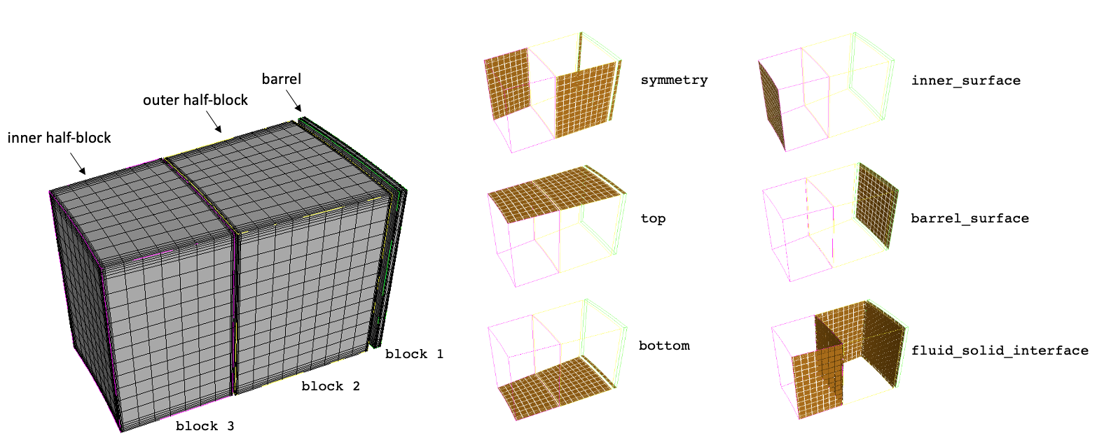
Figure 2: Solid mesh for the reflector blocks and barrel and a subset of the boundary names, before a series of mesh refinements
Unique boundary names are set for each boundary to which we will apply a unique boundary condition; we define the boundaries on the top and bottom of the block, the symmetry boundaries that reflect the fact that we've reduced the full PB-FHR reflector to a half-block domain, and boundaries at the interface between the reflector and the bed and on the barrel surface. The boundary that contains all fluid-solid interfaces through which we will exchange heat flux and temperature is named fluid_solid_interface.
Now that the overall structure of the mesh has been introduced, a brief description of the process of how the mesh was actually constructed is provided. First, the block geometry is formed by creating cylinders and bricks and subtracting them from one another to get angular sectors of cylindrical annuli. Then, the Cubit boundary_layer feature is used to programmatically refine the mesh near surfaces; we perform this refinement because, on some of these surfaces (those exchanging heat with the fluid), we expect to have higher thermal gradients that we would like to resolve with a finer mesh. For each boundary layer, we specify a starting element width perpendicular to the surface, a growth factor, and a number of boundary layers we would like to mesh. Finally, the mesh is saved in Exodus II format to disk.
Fluid nekRS Mesh
The fluid.jou is a Cubit script that is used to generate the fluid mesh, shown below.
#!python

# This is a mesh of 1/24th of the fluid in the outer reflector ring in the KP-FHR (there are 24
# blocks per ring). Only the fluid phase is modeled.

import math

# multiplicative factor to apply to the gap width; the nominal gap width cited
# in Shaver et. al (2019) corresponds to a gap amplification factor of 1.0.
gap_amplification = 3

# Path to the virtual_test_bed repository on your computer
directory = '/Users/anovak/projects/virtual_test_bed/'

core_radius       = 2.6
layer1_thickness  = 0.3
layer2_thickness  = 0.4
block_gap         = 0.002 * gap_amplification
bypass_gap        = 0.02
height            = 0.502
barrel_thickness  = 0.022
n_blocks_per_ring = 24
angle             = 360 / n_blocks_per_ring

barrel_outer_radius = core_radius + layer1_thickness + block_gap + layer2_thickness +\
  bypass_gap + barrel_thickness
barrel_inner_radius = barrel_outer_radius - barrel_thickness

layer2_outer_radius = barrel_inner_radius - bypass_gap
layer2_inner_radius = layer2_outer_radius - layer2_thickness

layer1_outer_radius = layer2_inner_radius - block_gap
layer1_inner_radius = layer1_outer_radius - layer1_thickness

porous_outer_radius = layer1_inner_radius
porous_inner_radius = porous_outer_radius - 3e-2

cubit.cmd('create cylinder radius ' + str(layer2_outer_radius) + ' height ' + str(height))
cubit.cmd('create cylinder radius ' + str(layer2_inner_radius) + ' height ' + str(height))
cubit.cmd('subtract volume 2 from volume 1')
cubit.cmd('compress all')
cubit.cmd('merge all')

cubit.cmd('create cylinder radius ' + str(layer1_outer_radius) + ' height ' + str(height))
cubit.cmd('create cylinder radius ' + str(layer1_inner_radius) + ' height ' + str(height))
cubit.cmd('subtract volume 3 from volume 2 keep')
cubit.cmd('delete volume 2')
cubit.cmd('compress all')
cubit.cmd('merge all')

# create the porous region
cubit.cmd('create cylinder radius ' + str(porous_inner_radius) + ' height ' + str(height))
cubit.cmd('subtract volume 4 from volume 2')
cubit.cmd('compress all')
cubit.cmd('merge all')

cubit.cmd('create brick x ' + str(2.0 * barrel_outer_radius) + ' y ' + str(barrel_outer_radius) + ' z ' + str(height))
cubit.cmd('move volume 4 y ' + str(-barrel_outer_radius / 2.0))
cubit.cmd('subtract volume 4 from volume 1 3')
cubit.cmd('compress all')
cubit.cmd('merge all')

cubit.cmd('create brick x ' + str(2.0 * barrel_outer_radius) + ' y ' + str(barrel_outer_radius) + ' z ' + str(height))
cubit.cmd('move volume 4 y ' + str(barrel_outer_radius / 2.0))
cubit.cmd('rotate volume 4 angle ' + str(angle) + ' about Z include_merged')
cubit.cmd('subtract volume 4 from volume 1 3')
cubit.cmd('compress all')
cubit.cmd('merge all')

cubit.cmd('create cylinder radius ' + str(barrel_outer_radius) + ' height ' + str(height))
cubit.cmd('create cylinder radius ' + str(barrel_inner_radius) + ' height ' + str(height))
cubit.cmd('subtract volume 5 from volume 4')
cubit.cmd('compress all')
cubit.cmd('merge all')

cubit.cmd('rotate Volume 1 angle ' + str(-angle / 2.0) + ' about origin 0 0 0 direction 0 0 1')

# create a block of fluid
cubit.cmd('create cylinder radius ' + str(barrel_outer_radius) + ' height ' + str(height))
cubit.cmd('create cylinder radius ' + str(layer1_inner_radius) + ' height ' + str(height))
cubit.cmd('subtract volume 6 from volume 5')
cubit.cmd('compress all')
cubit.cmd('merge all')

# size of gap between adjacent blocks in this model
l = block_gap / 2.0
cubit.cmd('create brick x ' + str(2.0 * barrel_outer_radius) + ' y ' + str(2.0 * barrel_outer_radius) + ' z ' + str(height))
cubit.cmd('move volume 6 y ' + str(-barrel_outer_radius - l))
cubit.cmd('subtract volume 6 from volume 2 4 5')
cubit.cmd('compress all')
cubit.cmd('merge all')

theta = (90.0 - angle / 2.0) * math.pi / 180.
cubit.cmd('create brick x ' + str(2.0 * barrel_outer_radius) + ' y ' + str(2.0 * barrel_outer_radius) + ' z ' + str(height))
cubit.cmd('move volume 6 y ' + str(barrel_outer_radius))
cubit.cmd('rotate volume 6 angle ' + str(angle / 2.0) + ' about Z include_merged')
cubit.cmd('move volume 6 x ' + str(-l * math.cos(theta)) + ' y ' + str(l * math.sin(theta)) + ' about Z include_merged')
cubit.cmd('subtract volume 6 from volume 2 4 5')
cubit.cmd('compress all')
cubit.cmd('merge all')

cubit.cmd('subtract volume 1 3 4 from volume 5')
cubit.cmd('compress all')
cubit.cmd('merge all')

cubit.cmd('subtract volume 2 from volume 1 imprint keep')
cubit.cmd('merge all')
cubit.cmd('compress all')
cubit.cmd('delete volume 1')
cubit.cmd('merge all')
cubit.cmd('compress all')

# now, create extra volumes just so that I have internal surfaces that I can
# use to control boundary layers
cubit.cmd('create brick x ' + str(2.0 * barrel_outer_radius) + ' y ' + str(2.0 * barrel_outer_radius) + ' z ' + str(height))
cubit.cmd('move volume 3 y ' + str(-barrel_outer_radius))
cubit.cmd('subtract volume 3 from volume 2 keep')
cubit.cmd('delete volume 3')
cubit.cmd('subtract volume 4 from volume 2 keep')
cubit.cmd('delete volume 2')
cubit.cmd('compress all')
cubit.cmd('merge all')

cubit.cmd('create cylinder radius ' + str(layer1_outer_radius) + ' height ' + str(height))
cubit.cmd('create cylinder radius ' + str(layer1_inner_radius) + ' height ' + str(height))
cubit.cmd('subtract volume 5 from volume 4')
cubit.cmd('compress all')
cubit.cmd('merge all')

cubit.cmd('subtract volume 4 from volume 1 imprint keep')
cubit.cmd('delete volume 4')
cubit.cmd('subtract volume 5 from volume 1 imprint keep')
cubit.cmd('delete volume 1')
cubit.cmd('compress all')
cubit.cmd('merge all')
cubit.cmd('imprint volume 1 2 3 4')

cubit.cmd('create cylinder radius ' + str(layer2_outer_radius) + ' height ' + str(height))
cubit.cmd('create cylinder radius ' + str(layer2_inner_radius) + ' height ' + str(height))
cubit.cmd('subtract volume 6 from volume 5')
cubit.cmd('compress all')
cubit.cmd('merge all')
cubit.cmd('subtract volume 5 from volume 3 keep')
cubit.cmd('delete volume 5')
cubit.cmd('split body 6')
cubit.cmd('subtract volume 6 7 from volume 3 keep')
cubit.cmd('delete volume 3')
cubit.cmd('compress all')
cubit.cmd('merge all')
cubit.cmd('imprint volume 1 2 3 4 5 6')

cubit.cmd('create cylinder radius ' + str(layer2_inner_radius) + ' height ' + str(height))
cubit.cmd('create cylinder radius ' + str(layer1_outer_radius) + ' height ' + str(height))
cubit.cmd('subtract volume 8 from volume 7')
cubit.cmd('create brick x ' + str(2.0 * barrel_outer_radius) + ' y ' + str(2.0 * barrel_outer_radius) + ' z ' + str(height))
cubit.cmd('move volume 9 y ' + str(-barrel_outer_radius))
cubit.cmd('subtract volume 9 from volume 7')
cubit.cmd('compress all')
cubit.cmd('merge all')

cubit.cmd('create brick x ' + str(2.0 * barrel_outer_radius) + ' y ' + str(2.0 * barrel_outer_radius) + ' z ' + str(height))
cubit.cmd('move volume 8 y ' + str(barrel_outer_radius))
cubit.cmd('rotate volume 8 angle ' + str(angle / 2.0) + ' about Z include_merged')
cubit.cmd('subtract volume 8 from volume 7 5 keep')
cubit.cmd('delete volume 8')
cubit.cmd('subtract volume 7 from volume 4 keep')
cubit.cmd('delete volume 7')
cubit.cmd('subtract volume 10 from volume 5 keep')
cubit.cmd('subtract volume 9 from volume 4 keep')
cubit.cmd('split body 13')
cubit.cmd('delete volume 4 5 14')
cubit.cmd('compress all')
cubit.cmd('merge all')
cubit.cmd('compress all')

cubit.cmd('delete volume 1 2')
cubit.cmd('merge all')
cubit.cmd('compress all')

cubit.cmd('block 1 volume 1 2 3 4 5 6 7')

surfaces = ''
for i in range(1, 36 + 1):
  surfaces += str(i) + ' '

cubit.cmd('surface ' + surfaces + ' size ' + str(block_gap))

gap_layer1 = 2e-4

# create boundary layers on all the surfaces - first, do the ones that naturally have corners
cubit.cmd('create boundary_layer 1')
cubit.cmd('modify boundary_layer 1 uniform height ' + str(gap_layer1) + ' growth 1.2 layers 4')
cubit.cmd('modify boundary_layer 1 add surface 23 volume 4 surface 30 volume 6')

cubit.cmd('create boundary_layer 2')
cubit.cmd('modify boundary_layer 2 uniform height ' + str(gap_layer1) + ' growth 1.2 layers 4')
cubit.cmd('modify boundary_layer 2 add surface 32 volume 6 surface 9 volume 2 surface 36 volume 7')

cubit.cmd('create boundary_layer 3')
cubit.cmd('modify boundary_layer 3 uniform height ' + str(gap_layer1) + ' growth 1.2 layers 4')
cubit.cmd('modify boundary_layer 3 add surface 28 volume 5 surface 6 volume 1')

# boundary layers on internal solid surfaces
cubit.cmd('create boundary_layer 5')
cubit.cmd('modify boundary_layer 5 uniform height ' + str(gap_layer1) + ' growth 1.2 layers 4')
cubit.cmd('modify boundary_layer 5 add surface 21 volume 4 surface 7 volume 6 surface 19 volume 6 surface 12 volume 2  surface 13 volume 7 surface 10 volume 7 surface 17 volume 3 surface 25 volume 5 surface 33 volume 7 surface 15 volume 3 surface 2 volume 5 surface 16 volume 5 surface 5 volume 1 surface 1 volume 1')

# "approach" boundary layers
cubit.cmd('create boundary_layer 6')
cubit.cmd('modify boundary_layer 6 uniform height ' + str(gap_layer1) + ' growth 1.6 layers ' + str(10 / uniform_refine))
cubit.cmd('modify boundary_layer 6 add surface 19 volume 4 surface 7 volume 2 surface 10 volume 2 surface 13 volume 3 surface 16 volume 3 surface 2 volume 1')

cubit.cmd('create boundary_layer 7')
cubit.cmd('modify boundary_layer 7 uniform height ' + str(gap_layer1 * 2) + ' growth 1.6 layers ' + str(6 / uniform_refine))
cubit.cmd('modify boundary_layer 7 add surface 4 volume 1 surface 11 volume 2 surface 18 volume 3 surface 20 volume 4 surface 26 volume 5 surface 31 volume 6 surface 34 volume 7')

cubit.cmd('create boundary_layer 8')
cubit.cmd('modify boundary_layer 8 uniform height ' + str(gap_layer1 * 2) + ' growth 1.6 layers ' + str(6 / uniform_refine))
cubit.cmd('modify boundary_layer 8 add surface 3 volume 1 surface 8 volume 2 surface 14 volume 3 surface 24 volume 4 surface 27 volume 5 surface 29 volume 6 surface 35 volume 7')

cubit.cmd('mesh volume 1 2 3 4 5 6 7')
cubit.cmd('block 1 element type HEX20')

# unite all the subblocks used just for the sake of controlling boundary layers
cubit.cmd('unite volume 1 2 3 4 5 6 7 include_mesh')
cubit.cmd('compress all')
cubit.cmd('merge all')

cubit.cmd('block 1 volume 1')

cubit.cmd('sideset 1 surface 7 5 9')
cubit.cmd('sideset 1 name "outer_block_surface"')

cubit.cmd('sideset 2 surface 2 6')
cubit.cmd('sideset 2 name "inner_block_surface"')

cubit.cmd('sideset 3 surface 3 10')
cubit.cmd('sideset 3 name "lower_symmetry"')

cubit.cmd('sideset 4 surface 4')
cubit.cmd('sideset 4 name "upper_symmetry"')

cubit.cmd('sideset 5 surface 8')
cubit.cmd('sideset 5 name "bottom_gaps"')

cubit.cmd('sideset 6 surface 12')
cubit.cmd('sideset 6 name "top_gaps"')

cubit.cmd('sideset 7 surface 11')
cubit.cmd('sideset 7 name "barrel_surface"')

cubit.cmd('sideset 8 surface 1')
cubit.cmd('sideset 8 name "porous_inner_surface"')

cubit.cmd('set large exodus file on')
cubit.cmd('export Genesis "' + directory + "pbfhr/reflector/meshes/" + 'fluid.exo" dimension 3 overwrite')
The complete fluid mesh is shown below; the boundary names are illustrated towards the right by showing only the highlighted surface to which each boundary corresponds. Names are shown in Courier font. While the names of the surfaces are shown in Courier font, nekRS does not directly use these names - rather, nekRS assigns boundary conditions based on the numeric value of the boundary name; these are shown as "ID" in the figure. An important restriction in nekRS is that the boundary IDs be ordered sequentially beginning from 1.
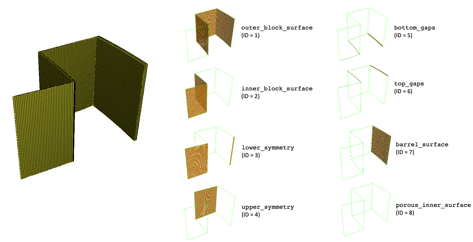
Figure 3: Fluid mesh for the FLiBe flowing around the reflector blocks, along with boundary names and IDs. It is difficult to see, but the porous_inner_surface boundary corresponds to the thin surface at the interface between the reflector region and the pebble bed.
A strength of Cardinal for conjugate heat transfer applications is that the fluid and solid meshes do not need to share nodes on a common surface; libMesh mesh-to-mesh data interpolations apply to surfaces of very different refinement and position in space; meshes may even overlap, such as for curvilinear applications. Figure 4 shows a zoom-in of the two mesh files (for the fluid and solid phases); rather than being limited with a continuous mesh mapping from the fluid phase inwards to the solid phase, each phase can be meshed according to its physics requirements.
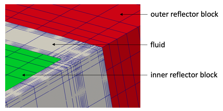
Figure 4: Zoomed-in view of the fluid and solid meshes, overlaid in Paraview. Lines are element boundaries.
Creating the fluid mesh is significantly more involved than creating the solid mesh. First, a series of boolean operations is performed to obtain an un-meshed volume that the fluid will flow through. Rather than create a single volume, the fluid region is created as 7 separate volumes; this allows full customzation of the meshing near the corners where we would like the boundary layer scheme to extend from the interior corners (with angles greater than 180 degrees) across the fluid gaps. Like the solid mesh, boundary layers are applied on all surfaces (even if the particular boundary condition on a surface is not necessarily "no-slip"). Finally, the boundary IDs are created; while names are assigned in the Cubit script, these names are not accessible to nekRS, and the numeric boundary IDs are instead used for designating boundaries.
Because nekRS uses a custom binary mesh format with a .re2 extension, a conversion utility must be used to convert an Exodus II format to nekRS's .re2 nekRS format. This utility, or the exo2nek program, requires the Exodus mesh elements to be type HEX20 (a twenty-node hexahedral element), so we set this element type from Cubit. Instructions for building the exo2nek program are available here. After this script has been compiled, you simply need to run
$ exo2nek
and then follow the prompts for the information that must be added about the mesh to perform the conversion. Above, $ indicates the terminal prompt. For this example, there is no solid mesh, there are no periodic surface pairs, and we want a scaling factor of (for the non-dimensional formulation) and no translation. The last part of the exo2nek program will request a name for the fluid .re2 mesh; providing fluid then will create the nekRS mesh, named fluid.re2.
Part 1: Initial Conduction Coupling
In this section, nekRS and MOOSE are coupled for conduction heat transfer in the solid reflector blocks and barrel, and through a stagnant fluid. The purpose of this stage of the analysis is to obtain a restart file for use as an initial condition in Part 2: Conjugate Heat Transfer Coupling to accelerate the nekRS calculation for conjugate heat transfer, since the energy equation is slowest to converge.
All input files for this stage of the analysis are present in the pbfhr/reflector/conduction directory. The following sub-sections describe these files.
Solid Input Files
The solid phase is solved with the MOOSE heat conduction module, and are described in the solid.i input. At the top of this file, the core heat flux is defined as a variable local to the file.
################################################################################
## FHR bypass flow in outer reflector                                         ##
## Cardinal Main Application                                                  ##
## Heat conduction in solid phase                                             ##
## POC : anovak at anl.gov                                                    ##
################################################################################
# If using or referring to this model, please cite as explained in
# https://mooseframework.inl.gov/virtual_test_bed/citing.html

# core average heat flux from the pebbles to the blocks
core_heat_flux = 5e3

[GlobalParams]
  # Reduces transfers efficiency for now, can be removed once transferred fields are checked
  bbox_factor = 10
[]

# Note: the mesh is stored using git large file system (LFS)The value of this variable can then be used anywhere else in the input file with syntax like ${core_heat_flux}, similar to bash syntax. Next, the solid mesh is specified by pointing to the Exodus mesh generated in Solid MOOSE Heat Conduction Mesh .
[Mesh]
  type = FileMesh
  file = ../meshes/solid.e
[]The heat conduction module will solve for temperature, which is defined as a nonlinear variable.
[Variables]
  [T]
  []
[]The Transfer system in MOOSE is used to communicate auxiliary variables across applications; a boundary heat flux will be computed by MOOSE and applied as a boundary condition in nekRS. In the opposite direction, nekRS will compute a surface temperature that will be applied as a boundary condition in MOOSE. Therefore, both the flux (flux) and surface temperature (nek_temp) are declared as auxiliary variables. The solid app will compute flux, while nek_temp will simply receive a solution from the nekRS sub-application. The flux is computed as a constant monomial field (a single value per element) due to the manner in which material properties are accessible in auxiliary kernels in MOOSE.
[AuxVariables]
  [flux]
    family = MONOMIAL
    order = CONSTANT
  []
  [nek_temp]
  []
[]In this example, the overall calculation workflow is as follows:
Run MOOSE heat conduction with a given surface temperature distribution from nekRS.
Send heat flux to nekRS as a boundary condition.
Run nekRS with a given surface heat flux distribution from MOOSE.
Send surface temperature to MOOSE as a boundary condition.
The above sequence is repeated until convergence of the coupled domain. For the very first time step, an initial condition should be set for nek_temp; this is done using a function with an arbitrary, but not wholly unrealistic, distribution for the fluid temperature. That function is then used as an initial condition with a FunctionIC object.
[Functions]
  [nek_temp_ic]
    type = ParsedFunction
    expression = 923.0-50.0*(r-3.348)
    symbol_names = 'r'
    symbol_values = 'r'
  []
  [r]
    type = ParsedFunction
    expression = sqrt(x*x+y*y)
  []
[]

[ICs]
  [nek_temp]
    type = FunctionIC
    variable = nek_temp
    function = nek_temp_ic
  []
[]Next, the governing equation solved by MOOSE is specified with the Kernels block as the HeatConduction kernel, or . An auxiliary kernel is also specified for the flux variable that specifies that the flux on the fluid_solid_interface boundary should be computed as .
[Kernels]
  [conduction]
    type = HeatConduction
    variable = T
  []
[]

[AuxKernels]
  [flux]
    type = DiffusionFluxAux
    variable = flux
    diffusion_variable = T
    component = normal
    check_boundary_restricted = false
    diffusivity = thermal_conductivity
    boundary = 'fluid_solid_interface'
  []
[]Next, the boundary conditions on the solid are applied. On the fluid-solid interface, a MatchedValueBC applies the value of the nek_temp receiver auxiliary variable to T in a strong Dirichlet sense. Insulated boundary conditions are applied on the symmetry, top, and bottom boundaries. On the boundary at the bed-reflector interface, the core heat flux is specified as a NeumannBC. Finally, on the surface of the barrel, a heat flux of is specified, where both and are specified as material properties.
[BCs]
  [cht_interface]
    type = MatchedValueBC
    variable = T
    v = nek_temp
    boundary = 'fluid_solid_interface'
  []
  [insulated]
    type = NeumannBC
    variable = T
    boundary = 'symmetry top bottom'
    value = 0.0
  []
  [inner_surface]
    type = NeumannBC
    variable = T
    value = ${core_heat_flux}
    boundary = 'inner_surface'
  []
  [outer_surface]
    type = ConvectiveHeatFluxBC
    variable = T
    T_infinity = 'Tinf'
    heat_transfer_coefficient = 'htc'
    boundary = 'barrel_surface'
  []
[]The HeatConduction kernel requires a material property for the thermal conductivity; material properties are also required for the heat transfer coefficient and far-field temperature for the ConvectiveHeatFluxBC. These material properties are specified in the Materials block. Here, different values for thermal conductivity are used in the graphite and steel.
[Materials]
  [k_graphite]
    type = GenericConstantMaterial
    prop_names = 'thermal_conductivity'
    prop_values = '43.73' # evaluated at 650 C
    block = '2 3'
  []
  [k_steel]
    type = GenericConstantMaterial
    prop_names = 'thermal_conductivity'
    prop_values = '23.82' # evaluated at 650 C
    block = '1'
  []
  [htc_and_Tinf]
    type = GenericConstantMaterial
    prop_names = 'htc Tinf'
    prop_values = '10.0 300.0'
  []
[]Next, the MultiApps and Transfers blocks describe the interaction between Cardinal and MOOSE. The MOOSE heat conduction module is here run as the main application, with the nekRS wrapping run as the sub-application. We specify that MOOSE will run first on each time step. Allowing sub-cycling means that, if the MOOSE time step is 0.05 seconds, but the nekRS time step is 0.02 seconds, that for every MOOSE time step, nekRS will perform three time steps, of length 0.02, 0.02, and 0.01 seconds to "catch up" to the MOOSE main application. If sub-cycling is turned off, then the smallest time step among all the various applications is used.
Three transfers are required to couple Cardinal and MOOSE; the first is a transfer of surface temperature from Cardinal to MOOSE. The second is a transfer of heat flux from MOOSE to Cardinal. And the third is a transfer of the total integrated heat flux from MOOSE to Cardinal (computed as a postprocessor), which is then used internally by nekRS to re-normalize the heat flux (after interpolation onto its Gauss-Lobatto-Legendre (GLL) points).
[MultiApps]
  [nek]
    type = TransientMultiApp
    app_type = CardinalApp
    input_files = 'nek.i'
    sub_cycling = true
    execute_on = timestep_end
  []
[]

[Transfers]
  [temperature_from_nek]
    type = MultiAppGeneralFieldNearestLocationTransfer
    source_variable = temp
    from_multi_app = nek
    variable = nek_temp
  []
  [flux_to_nek]
    type = MultiAppGeneralFieldNearestLocationTransfer
    source_variable = flux
    to_multi_app = nek
    variable = avg_flux
    source_boundary = 'fluid_solid_interface'
  []
  [flux_integral_to_nek]
    type = MultiAppPostprocessorTransfer
    to_postprocessor = flux_integral
    from_postprocessor = flux_integral
    to_multi_app = nek
  []
[]For transfers between two native MOOSE applications, you can ensure conservation of a transferred field using the from_postprocessors_to_be_preserved and to_postprocessors_to_be_preserved options available to any class inheriting from MultiAppConservativeTransfer. However, proper conservation of a field within nekRS (which uses a completely different spatial discretization from MOOSE) requires performing such conservations in nekRS itself. Hence, an integral postprocessor must explicitly be passed in this case.
Next, postprocessors are used to compute the integral heat flux as a SideIntegralVariablePostprocessor.
[Postprocessors]
  [flux_integral]
    type = SideIntegralVariablePostprocessor
    variable = flux
    boundary = 'fluid_solid_interface'
  []
[]Next, the solution methodology is specified. Although the solid phase only includes time-independent kernels, the heat conduction is run as a transient because nekRS ultimately must be run as a transient (nekRS lacks a steady solver). A nonlinear tolerance of is used for each solid time step, and the overall coupled simulation is considered converged once the relative change in the solution between steps is less than . Finally, an output format of Exodus II is specified.
[Executioner]
  type = Transient
  dt = 0.005
  nl_abs_tol = 1e-6
  num_steps = 2000

  steady_state_detection = true
  steady_state_tolerance = 5e-4
[]

[Outputs]
  exodus = true
  print_linear_residuals = false
[]Fluid Input Files
The fluid phase is solved with Cardinal, which under-the-hood performs the solution with nekRS. The wrapping of nekRS as a MOOSE application is specified in the nek.i file. Compared to the solid input file, the fluid input file is quite minimal, as the specification of the nekRS problem setup is mostly performed using the nekRS input files that would be required to run nekRS as a standalone application.
First, a local variable, fluid_solid_interface, is used to define all the boundary IDs through which nekRS is coupled via conjugate heat transfer to MOOSE for convenience. Next, a NekRSMesh, a class specific to Cardinal, is used to construct a "mirror" of the surfaces in the nekRS mesh through which boundary condition coupling is performed. In order for MOOSE's MultiAppGeneralFieldNearestLocationTransfer to correctly match nodes in the solid mesh to nodes in this fluid mesh mirror, the entire mesh must be scaled by a factor of to return to dimensional units.
################################################################################
## FHR bypass flow in outer reflector                                         ##
## Cardinal Sub Application to run NekRS                                      ##
## 3D RANS model                                                              ##
## POC : anovak at anl.gov                                                    ##
################################################################################
# If using or referring to this model, please cite as explained in
# https://mooseframework.inl.gov/virtual_test_bed/citing.html

fluid_solid_interface = '1 2 7'

# Note: the mesh is stored using git large file system (LFS)
[Mesh]
  type = NekRSMesh
  boundary = ${fluid_solid_interface}
  scaling = 0.006
[]Next, the Problem block describes all objects necessary for the actual physics solve; for the solid input file, the default of FEProblem was implicitly assumed. However, to replace MOOSE finite element calculations with nekRS spectral element calculations, a Cardinal-specific NekRSProblem class is used. Like all MOOSE-wrapped apps, the problem class that wraps nekRS derives from ExternalProblem. To allow conversion between a non-dimensional nekRS solve and a dimensional MOOSE coupled heat conduction application, the characteristic scales used to establish the non-dimensional problem are provided.
[Problem]
  type = NekRSProblem
  casename = 'fluid'
  n_usrwrk_slots = 1

  [FieldTransfers]
    [avg_flux]
      type = NekBoundaryFlux
      direction = to_nek
      usrwrk_slot = 0
      postprocessor_to_conserve = flux_integral
    []
    [temp]
      type = NekFieldVariable
      direction = from_nek
      field = temperature
    []
  []

  [Dimensionalize]
    L = 0.006
    U = 0.0575
    T = 923.15
    dT = 10.0
    rho = 1962.13
    Cp = 2416.0
  []
[]Next, a Transient executioner is specified. This is the same executioner used for the solid case, except now a Cardinal-specific time stepper, NekTimeStepper is provided. This time stepper simply reads the time step specified in nekRS's .par file (to be described shortly), and converts it to dimensional form if needed. An Exodus II output format is specified. It is important to note that this output file only outputs the temperature and heat flux solutions on the surface mirror mesh; the solution over the entire nekRS domain is output with the usual .fld field file format used by standalone nekRS calculations.
[Executioner]
  type = Transient

  [TimeStepper]
    type = NekTimeStepper
  []
[]

[Outputs]
  exodus = true
[]Finally, several postprocessors are included. A postprocessor named flux_integral is added automatically by NekRSProblem to receive the value of the heat flux integral from MOOSE for internal normalization in nekRS. The other three postprocessors are all Cardinal-specific postprocessors that perform integrals and global min/max calculations over the nekRS domain. Here, the boundary_flux postprocessor computes over a boundary in the nekRS mesh. This value should approximately match the imposed heat flux, flux_integral, though perfect agreement is not to be expected since flux boundary conditions are only weakly imposed in the spectral element method. The max_nek_T and min_nek_T then compute the maximum and minimum temperatures throughout the entire nekRS domain (i.e. not only on the conjugate heat transfer coupling surfaces).
[Postprocessors]
  [boundary_flux]
    type = NekHeatFluxIntegral
    boundary = ${fluid_solid_interface}
  []
  [max_nek_T]
    type = NekVolumeExtremeValue
    field = temperature
    value_type = max
  []
  [min_nek_T]
    type = NekVolumeExtremeValue
    field = temperature
    value_type = min
  []
[]Note that fluid.re2 does not appear anywhere in nek.i - the fluid.re2 file is a mesh used directly by nekRS, while NekRSMesh is a mirror of the boundaries in fluid.re2 through which boundary coupling with MOOSE will be performed.
You will likely notice that many of the almost-always-included MOOSE blocks are absent from the nek.i input file - for instance, there are no nonlinear or auxiliary variables. The NekRSProblem assists in input file setup by declaring many of these coupling fields automatically. For this example, two auxiliary variables named temp and avg_flux are added automatically; these variables receive incoming and outgoing transfers to/from nekRS. You will see both temp and avg_flux referred to in the solid input file Transfers section.
In addition, the nek.i input file only describes how nekRS is wrapped within the MOOSE framework; with the fluid.re2 mesh file, each nekRS simulation requires at least three additional files, that share the same case name fluid but with different extensions. The additional nekRS files are:
fluid.par: High-level settings for the solver, boundary condition mappings to sidesets, and the equations to solve.fluid.udf: User-defined C++ functions for on-line postprocessing and model setupfluid.oudf: User-defined OCCA kernels for boundary conditions and source terms
A detailed description of all of the available parameters, settings, and use cases for these input files is available on the nekRS documentation website. Because the purpose of this analysis is to demonstrate Cardinal's capabilties, only the aspects of nekRS required to understand the present case will be covered. First, begin with the fluid.par file, shown in entirety below.
# Input of solid conduction through FLiBe in the outer reflector block fluid region.
# Material properties are taken for FLiBe at 650 C.

# The problem is run in nondimensional form with the following characteristic scales:
# L_ref  = 0.006    (the width of the smallest block-block gap)
# V_ref  = 0.0575   (velocity needed to get the specified Reynolds number)
# T_ref  = 923.15   (the inlet temperature)
# dT_ref = 10.0     (arbitrary temperature range value)
# t_ref  = 0.1043   (reference time scale)
# rho_0  = 1962.13
# mu_0   = 6.77e-3
# Cp_0   = 2416
# k_0    = 1.09
# Pr     = 15.005

[GENERAL]
  stopAt = numSteps
  numSteps = 2000
  dt = 0.025
  timeStepper = tombo2
  writeControl = steps
  writeInterval = 100
  polynomialOrder = 2

[VELOCITY]
  solver = none

[PRESSURE]

[TEMPERATURE]
  conductivity = -1500.5
  rhoCp = 1.0
  residualTol = 1.0e-8
  boundaryTypeMap = f, f, I, I, t, o, f, I
The input consists of blocks and parameters. The [GENERAL] block describes the time stepping, simulation end control, and the polynomial order. Here, a time step of 0.025 (non-dimensional) is used; a nekRS output file is written every 100 time steps. Because nekRS is run as a sub-application to MOOSE, the stopAt and numSteps fields are actually ignored, so that the steady state tolerance in the MOOSE main application dictates when a simulation terminates. Because the purpose of this simulation is only to obtain a reasonable initial condition, a low polynomial order of 2 is used.
Next, the [VELOCITY] and [PRESSURE] blocks describe the solution of the pressure Poisson equation and velocity Helmholtz equations. In the velocity block, setting solver = none turns off the velocity solution; therefore, none of the parameters specified here are of consequence, so their description will be deferred to Part 2: Conjugate Heat Transfer Coupling . Finally, the [TEMPERATURE] block describes the solution of the temperature passive scalar equation. is set to unity because the solve is conducted in non-dimensional form, such that
(17)
The coefficient on the diffusive equation term, as shown in Eq. (12), is equal to . In nekRS, specifying conductivity = -1500.5 is equivalent to specifying conductivity = 0.00066644 (i.e. ), or a Peclet number of 1500.5.
Next, residualTol specifies the solver tolerance for the temperature equation to . Finally, the boundaryTypeMap is used to specify the mapping of boundary IDs to types of boundary conditions. nekRS uses short character strings to represent the type of boundary condition; boundary conditions used in this example include:
W: no-slip wallsymy: symmetry in the -directionv: user-defined velocityo: zero-gradient outletf: user-defined fluxI: insulatedt: user-defined temperature
Therefore, in reference to Figure 3, boundaries 1, 2, and 7 are flux boundaries (these boundaries will receive a heat flux from MOOSE), boundaries 3, 4, and 8 are insulated, boundary 5 is a specified temperature, and boundary 6 is a zero-gradient outlet. The actual assignment of numeric values to these boundary conditions is then performed in the fluid.oudf file. The fluid.oudf file contains OCCA kernels that will be run on a GPU (if present). Because this case does not have any user-defined source terms in nekRS, these OCCA kernels are only used to apply boundary conditions. The fluid.oudf file is shown below.
void scalarDirichletConditions(bcData * bc)
{
  if (bc->id == 5)
    bc->s = 0.0;
}

void scalarNeumannConditions(bcData * bc)
{
  if (bc->id == 1 || bc->id == 2 || bc->id == 7)
    bc->flux = bc->usrwrk[bc->idM];
}
The names of these functions correspond to the boundary conditions that were applied in the .par file - only the user-defined temperature and flux boundaries require user input in the .oudf file. For each function, the bcData object contains all information about the current boundary that is "calling" the function; bc->id is the boundary ID, bc->s is the scalar (temperature) solution at the present GLL point, and bc->flux is the flux (of temperature) at the present GLL point. The bc->usrwrk array is a scratch space to which the heat flux values coming from MOOSE are written. These OCCA functions then get called directly within nekRS.
Finally, the fluid.udf file contains C++ functions that are user-defined functions through which interaction with the nekRS solution are performed. Here, the UDF_Setup function is called once at the very start of the nekRS simulation, and it is here that initial conditions are applied. The fluid.udf file is shown below.
#include "udf.hpp"

void UDF_LoadKernels(occa::properties & kernelInfo)
{
}

void UDF_Setup(nrs_t *nrs)
{
  mesh_t * mesh = nrs->cds->mesh[0];

  // loop over all the GLL points and assign directly to the solution arrays by
  // indexing according to the field offset necessary to hold the data for each
  // solution component
  int n_gll_points = mesh->Np * mesh->Nelements;
  for (int n = 0; n < n_gll_points; ++n)
    nrs->cds->S[n] = 0;
}
The initial condition is applied manually by looping over all the GLL points and setting zero to each (recall that this is a non-dimensional simulation, such that corresponds to a dimensional temperature of ). Here, nrs->cds->S is the array holding the nekRS passive scalar solutions (of which there is only one for this example; for simulations with a - turbulence model, additional scalars would be present).
Execution and Postprocessing
To run the pseudo-steady conduction model, run the following from a command line or through a job submission script on a HPC system.
$ mpiexec -np 48 cardinal-opt -i solid.i
where mpiexec is an Message Passing Interface (MPI) compiler wrapper, -np 48 indicates that the input should be run with 48 processes, and -i solid.i specifies the input file to run in Cardinal. Both MOOSE and nekRS will be run with 48 processes.
When the simulation has completed, you will have created a number of different output files:
fluid0.f<n>, where<n>is a five-digit number indicating the output file number created by nekRS (a separate output file is written for each time step written to file according to the settings in thefluid.parfile). An extra program is required to visualize nekRS output files in Paraview; see the instructions here.solid_out.e, an Exodus II output file with the solid mesh and solution.solid_out_nek0.e, an Exodus II output file with the fluid mirror mesh and data that was ultimately transferred in/out of nekRS.
After converting the nekRS output files to a format viewable in Paraview, the simulation results can be displayed. The solid temperature, surface heat flux, and fluid temperature are shown below. Note that the fluid temperature is shown in nondimensional form based on the selected characteristic scales. The image of the fluid solution is rotated so as to better display the temperature variation around the inner reflector block. The domain shown in Figure 6 exactly corresponds to the "mirror" mesh constructed by NekRSMesh.
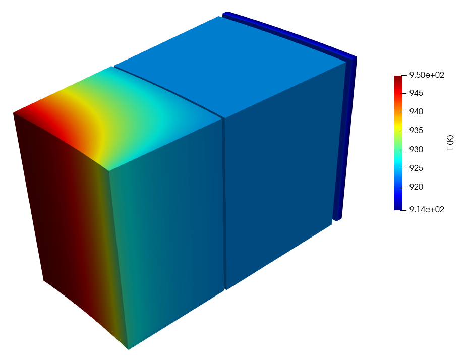
Figure 5: Solid temperature for steady state conduction coupling between MOOSE and nekRS
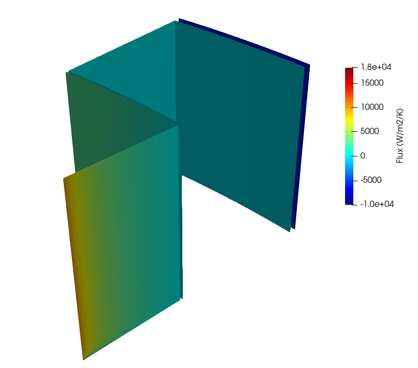
Figure 6: Solid surface heat flux for steady state conduction coupling between MOOSE and nekRS
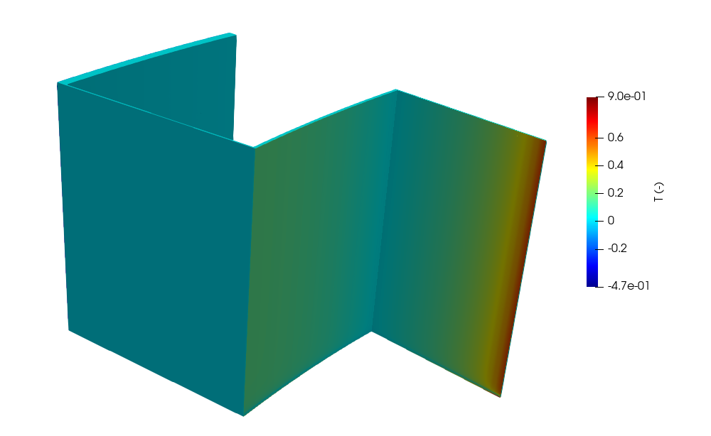
Figure 7: Fluid temperature (nondimensional) for steady state conduction coupling between MOOSE and nekRS
The solid blocks are heated by the pebble bed along the bed-reflector interface, so the temperatures are highest in the inner block. As can be seen in Figure 6, the heat flux into the fluid is in some places positive (such as near the inner reflector block) and is in other places negative (such as near the barrel) where heat leaves the system.
Part 2: Conjugate Heat Transfer Coupling
In this section, nekRS and MOOSE are coupled for conjugate heat transfer between the FLiBe coolant and the reflector blocks and barrel. All input files for this stage of the analysis are present in the pbfhr/reflector/cht directory. The following sub-sections describe all of these files; for brevity, most emphasis will be placed on input file setup that is different or extends the conduction case in Part 1: Initial Conduction Coupling .
Solid Input Files
The solid phase is again solved with the MOOSE heat conduction module. The input file is essentially the same as the conduction case, so is not discussed further.
Fluid Input Files
The fluid phase is again solved with nekRS wrapped as a MOOSE app via Cardinal. The input file is largely the same as the conduction case, except that additional postprocessors are added to query both the thermal and hydraulic aspects of the nekRS solution. The postprocessors used for the nekRS wrapping are shown below.
[Postprocessors]
  [boundary_flux]
    type = NekHeatFluxIntegral
    boundary = ${fluid_solid_interface}
  []
  [max_nek_T]
    type = NekVolumeExtremeValue
    field = temperature
    value_type = max
  []
  [min_nek_T]
    type = NekVolumeExtremeValue
    field = temperature
    value_type = min
  []
  [pressure_in]
    type = NekSideAverage
    field = pressure
    boundary = '5'
  []
  [mdot_in]
    type = NekMassFluxWeightedSideIntegral
    field = unity
    boundary = '5'
  []
  [mdot_out]
    type = NekMassFluxWeightedSideIntegral
    field = unity
    boundary = '6'
  []
[]We have added postprocessors to compute the average inlet pressure, and the average inlet and outlet mass flowrates. Like the NekVolumeExtremeValue, these postprocessors operate directly on nekRS's internal solution arrays to provide diagnostic information. Because the outlet pressure is set to zero, pressure_in corresponds to the pressure drop in the fluid.
As in Part 1: Initial Conduction Coupling , four additional files are required to set up the nekRS simulation - fluid.re2, fluid.par, fluid.udf, and fluid.oudf. These files are largely the same as those used in the steady conduction model, so only the differences will be emphasized here.
The fluid.par file is shown below. Here, startFrom provides a restart file, conduction.fld and specifies that we only want to read temperature from the file (by appending +T to the file name). We increase the polynomial order as well.
# Input of fluid flow of FLiBe in the outer reflector block fluid region.
# Material properties are taken for FLiBe at 650 C.

# The problem is run in nondimensional form with the following characteristic scales:
# L_ref  = 0.006    (the width of the smallest block-block gap)
# V_ref  = 0.0575   (velocity needed to get the specified Reynolds number)
# T_ref  = 923.15   (the inlet temperature)
# dT_ref = 10.0     (arbitrary temperature range value)
# t_ref  = 0.0208   (reference time scale)
# rho_0  = 1962.13
# mu_0   = 6.77e-3
# Cp_0   = 2416
# k_0    = 1.09
# Pr     = 15.005

# polynomialOrder was reduced from 4 to 3 for testing / CI purposes

[GENERAL]
  startFrom = conduction.fld+T
  stopAt = numSteps
  numSteps = 2000
  dt = 0.001
  timeStepper = tombo2
  writeControl = steps
  writeInterval = 100
  polynomialOrder = 3

[VELOCITY]
  viscosity = -100.0
  density = 1.0
  residualTol = 1.0e-8
  boundaryTypeMap = W, W, symy, W, v, o, W, W

[PRESSURE]
  residualTol = 1.0e-8

[TEMPERATURE]
  conductivity = -1500.5
  rhoCp = 1.0
  residualTol = 1.0e-8
  boundaryTypeMap = f, f, I, I, t, o, f, I
In the [VELOCITY] block, the density is set to unity, because the solve is conducted in nondimensional form, such that
(18)
The coefficient on the diffusive term, as shown in Eq. (11), is equal to . In nekRS, specifying diffusivity = -100.0 is equivalent to specifying diffusivity = 0.001 (i.e. ), or a Reynolds number of 100.0. All other parameters have similar interpretations as described in Part 1: Initial Conduction Coupling .
The fluid.udf file is shown below. The UDF_Setup function is again used to apply initial conditions; because temperature is read from the restart file, only initial conditions on velocity and pressure are required. nrs->U is an array storing the three components of velocity (padded with length nrs->fieldOffset), while nrs->P is the array storing the pressure solution. Due to the non-dimensional formulation, all values for the axial velocity are set to unity.
#include "udf.hpp"

void UDF_LoadKernels(occa::properties & kernelInfo)
{
  // Compute the inlet velocity boundary condition and propagate it to a kernel variable
  kernelInfo["defines/Vz"] = 1.0;

  // Compute the inlet temperature and propagate it to a kernel variable
  kernelInfo["defines/inlet_T"] = 0.0;
}

void UDF_Setup(nrs_t *nrs)
{
  mesh_t * mesh = nrs->cds->mesh[0];

  // loop over all the GLL points and assign directly to the solution arrays by
  // indexing according to the field offset necessary to hold the data for each
  // solution component
  int n_gll_points = mesh->Np * mesh->Nelements;
  for (int n = 0; n < n_gll_points; ++n)
  {
    nrs->U[n + 0 * nrs->fieldOffset] = 0.0; // x-velocity
    nrs->U[n + 1 * nrs->fieldOffset] = 0.0; // y-velocity
    nrs->U[n + 2 * nrs->fieldOffset] = 1.0; // z-velocity

    nrs->P[n] = 0.0; // pressure
  }
}
This file also includes the UDF_LoadKernels function, which is used to propagate quantities to variables accessibly through OCCA kernels. The kernelInfo object is used to define two variables - Vz and inlet_T that will be accessible through the GPU kernels, eliminating some burden on the user if the problem setup must be changed in multiple locations throughout the nekRS input files.
Finally, the fluid.oudf file is shown below. Because the velocity is enabled, additional boundary condition functions must be specified in addition to those in Part 1: Initial Conduction Coupling . The velocityDirichletConditions function applies Dirichlet conditions to velocity, where bc->u is the -component of velocity, bc->v is the -component of velocity, and bc->w is the -component of velocity. In this function, the kernel variable Vz that was defined in the fluid.udf file is accessible to simplify the boundary condition setup. The other boundary conditions, the Dirichlet temperature conditions and the Neumann heat flux conditions, are the same as for the steady conduction case.
void velocityDirichletConditions(bcData * bc)
{
  if (bc->id == 5)
  {
    bc->u = 0.0; // x-velocity
    bc->v = 0.0; // y-velocity
    bc->w = Vz;  // z-velocity
  }
}

void scalarDirichletConditions(bcData * bc)
{
  if (bc->id == 5)
    bc->s = inlet_T;
}

void scalarNeumannConditions(bcData * bc)
{
  if (bc->id == 1 || bc->id == 2 | bc->id == 7)
    bc->flux = bc->usrwrk[bc->idM];
}
Execution and Postprocessing
The instructions to run the conjugate heat transfer model are the same as those given in Execution and Postprocessing . The temperature and heat flux distributions are qualitatively quite similar to those in Part 1: Initial Conduction Coupling because temperature differences across the block gaps are not very large. Therefore, only the fluid pressure and velocity distributions are shown below, both in non-dimensional form.
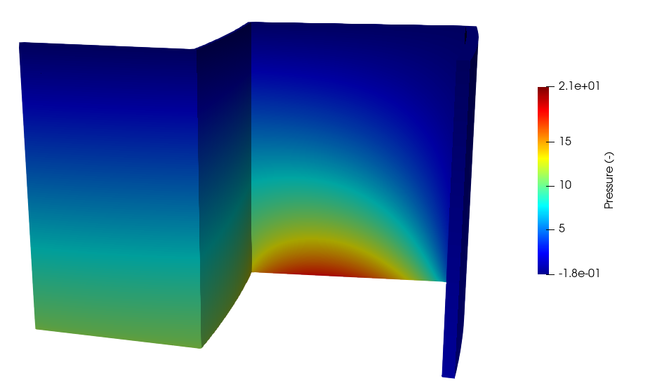
Figure 8: Pressure (nondimensional) for conjugate heat transfer coupling between MOOSE and nekRS
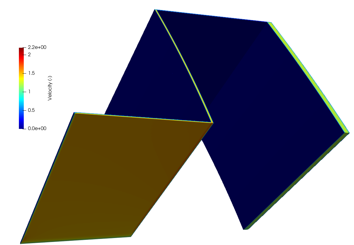
Figure 9: Velocity (nondimensional) for conjugate heat tranfser coupling between MOOSE and nekRS
The no-slip condition on the solid surface, and the symmetry condition on the surface, are clear in Figure 9. The pressure loss is highest in the gap along the boundary due to the imposition of no-slip conditions on both sides of the half-gap width due to limitations in nekRS's boundary conditions. Therefore, these pressure predictions are likely to change once nekRS's symmetry conditions are expanded to non-//-aligned surfaces.
Pronghorn Closures
This analysis has only predicted the conjugate heat transfer solution for a single value of Reynolds number and a single value of gap width. This section briefly describes the procedure necessary to use Cardinal for generating porous media closures for Pronghorn - specifically, the friction coefficient. Pronghorn's momentum conservation equation contains a distributed loss term Novak et al. (2020) that relates the friction pressure drop to a closure, ,
(19)
where is the porosity, is a diagonal tensor that is related to the conventional definition of a friction coefficient, and is the interstitial velocity. The present model can be used to predict as a function of the block geometry and the Reynolds number. The calculation workflow would be as follows:
Re-run the
solid.jouandfluid.jouscripts for a range of block gap widths.Re-run the steady conduction initial condition calculation in Part 1: Initial Conduction Coupling and the conjugate heat transfer calculation in Part 2: Conjugate Heat Transfer Coupling for the range of block gap widths, for a range of Reynolds numbers.
For each individual run, compute the overall porosity of the block-fluid domain, and express in Eq. (19) as , where is the pressure drop given by the
pressure_inpostprocessor in thenek.iinput file, and is the height of the block, or 0.52 m.Correlate the pressure drop results according to Eq. (19) and obtain a functional fit to (with terms linear and quadratic in velocity, according to dimensional considerations for pressure loss).
Use a
FunctionAnisotropicDragCoefficientsfriction factor model in Pronghorn, and provide the functional fit in the Pronghorn input file for the linear and quadratic terms inDarcy_coefficient(the linear proportionality) andForchheimer_coefficient(the quadratic proportionality).
An example showing this workflow for the PB-FHR (albeit with a significantly different reflector block geometry) using COMSOL is available in the literature Novak et al. (2021).
Similar calculation procedures would be used to predict the Nusselt number, or other porous media closures such as effective solid conductivities - parameterize the operating space and geometry that affects the physics of interest, run repeated high-resolution calculations, and correlate the data into a form that can then be inserted into Pronghorn using existing material property classes.
Acknowledgements
The Cardinal project is funded by the Nuclear Energy Advanced Modeling and Simulation (NEAMS) program, while nekRS is primarily funded through the Exascale Computing Project (ECP), with additional contributions from NEAMS.
References
- A.J. Novak, S. Schunert, R.W. Carlsen, P. Balestra, D. Andrs, J. Kelly, R.N. Slaybaugh, and R.C. Martineau.
Pronghorn Theory Manual.
2020.
URL: https://inldigitallibrary.inl.gov/sites/sti/sti/Sort_24425.pdf.[BibTeX]
- A.J. Novak, S. Schunert, R.W. Carlsen, P. Balestra, R.N. Slaybaugh, and R.C. Martineau.
Multiscale thermal-hydraulic modeling of the pebble bed fluoride-salt-cooled high-temperature reactor.
Annals of Nuclear Energy, 2021.
doi:10.1016/j.anucene.2020.107968.[BibTeX]
- H. Oehme and J. Schöning.
Design, Features and Engineering Status of the THTR 300 MWe Prototype Power Station.
Technical Report, Brown Boveri/Krupp Reaktorbau G.m.b.H., 1970.[BibTeX]
- D. Shaver, R. Hu, L. Zou, and E. Merzari.
Initial Industry Collaborations of the Center of Excellence.
Technical Report ANL/NSE-19/15, Argonne National Laboratory, 2019.
URL: https://www.osti.gov/biblio/1556071.[BibTeX]
- SNL.
CUBIT 13.2 User Documentation.
2012.
URL: https://tinyurl.com/rgsbqb7.[BibTeX]