MK1-FHR Plant Model
Contact: Guillaume Giudicelli, guillaume.giudicelli.at.inl.gov
Model link: FHR Plant Model
The multiphysics core model, which uses Griffin for neutronics and Pronghorn for coarse mesh porous media CFD, is coupled with the balance of plant model, which uses SAM for 1D thermal hydraulics of the primary and secondary loops.
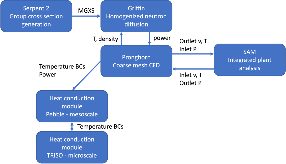
Coupling scheme for the Mk1-FHR plant model
Modifications to the core 2D-RZ model
The connection between the core model and the balance of plant simulation is made through the inlet and outlet of the core in the primary loop. Instead of a fixed inlet mass flow rate and a fixed outlet pressure like in the previous model, those quantities will be provided by the simulation of the rest of the primary loop.
The boundary information, collected in SAM, is passed between the applications using Transfers. In particular, the MultiAppPostprocessorsTransfer from SAM enables the transfer of multiple postprocessors by a single object.
[Transfers]
  [receive_flow_BCs]
    type = MultiAppPostprocessorVectorTransfer
    from_multi_app = primary
    from_postprocessors = 'Core_outlet_p Core_inlet_mdot Core_inlet_T'
    to_postprocessors = 'outlet_pressure inlet_mdot inlet_temp_fluid'
    # Initial execution is important to avoid using a default BC
    execute_on = 'INITIAL TIMESTEP_END'
  []
[]The outlet pressure is passed from SAM to Pronghorn and stored in a Receiver, as are the core inlet mass flow rate and temperature.
[Postprocessors]
  [inlet_mdot]
    type = Receiver
    default = 9.784508e+02 #${mfr}
    execute_on = 'INITIAL TIMESTEP_END TRANSFER'
  []

  [inlet_temp_fluid]
    type = Receiver
    default = 8.741515e+02 #${inlet_T_fluid}
    execute_on = 'INITIAL TIMESTEP_END TRANSFER'
  []

  [outlet_pressure]
    type = Receiver
    default = 1.865956e+05 #${outlet_pressure_val}
    execute_on = 'INITIAL TIMESTEP_END TRANSFER'
  []
[]The boundary conditions are modified appropriately to use the boundary information newly stored in those Postprocessors. Flux boundary conditions are utilized as they are naturally conservative in a finite volume method. The fluxes for the mass, momentum and energy equations are all provided, computed by the boundary conditions based on the mass flow rates, local density and inlet surface area.
    inlet_boundaries = 'bed_horizontal_bottom OR_horizontal_bottom'
    momentum_inlet_types = 'fixed-velocity fixed-velocity'
    momentum_inlet_function = '0 inlet_vel_y_fun; 0 0'
    energy_inlet_types = 'fixed-temperature heatflux'
    energy_inlet_function = 'T_inlet_fun 0'
    # so the flux BCs have to be used consistently across all equations

    # Outlet boundary conditions
    outlet_boundaries = 'bed_horizontal_top plenum_top OR_horizontal_top'
    momentum_outlet_types = 'fixed-pressure fixed-pressure fixed-pressure'
pressure_function = 'pressure_out_fun pressure_out_fun pressure_out_fun'In the other direction of the coupling, the boundary conditions that will be passed to SAM are collected using side integrals and flow rate postprocessors. These are executed at the end of each time step and collect the outlet flow conditions as well as the inlet pressure. The inlet temperature is also computed in case of a flow reversal.
[Postprocessors]
  [pressure_in]
    type = SideAverageValue
    boundary = 'bed_horizontal_bottom'
    variable = pressure
    execute_on = 'INITIAL TIMESTEP_END TRANSFER'
  []

  [mass_flow_out]
    type = VolumetricFlowRate
    boundary = 'bed_horizontal_top plenum_top OR_horizontal_top'
    advected_quantity = ${rho_fluid}
    execute_on = 'INITIAL TIMESTEP_END TRANSFER'
  []

  [T_flow_out]
    type = ParsedPostprocessor
    function = 'e_flow_out / mass_flow_out / cp_fluid'
    pp_names = 'e_flow_out mass_flow_out'
    constant_names = 'cp_fluid'
    constant_expressions = '2416'
    execute_on = 'INITIAL TIMESTEP_END TRANSFER'
  []

  [T_flow_in]
    type = ParsedPostprocessor
    function = '-e_flow_in_m / inlet_mdot / cp_fluid'
    pp_names = 'e_flow_in_m inlet_mdot'
    constant_names = 'cp_fluid'
    constant_expressions = '2416'
    execute_on = 'INITIAL TIMESTEP_END TRANSFER'
  []
[]The Transfer system is once again leveraged, this time to send data to SAM. The modifications to the SAM input are detailed in the next section.
[Transfers]
  [send_flow_BCs]
    type = MultiAppPostprocessorVectorTransfer
    to_multi_app = primary
    from_postprocessors = 'pressure_in mass_flow_out T_flow_out T_flow_in'
    to_postprocessors = 'Core_inlet_pressure Core_outlet_mdot Core_outlet_T Core_inlet_T_reversal'
  []
[]Modifications to the balance of plant 1D model
The initial SAM model of the Mk1-FHR models the entire primary and secondary loop as well as a selection of passive systems. A 1D model of the core is present in the primary loop, providing a heat source as well as estimating the coolant travel time in the core and the pressure drop from friction in the pebble bed. This 1D core component is removed in the coupled model, as it is replaced with a 2D RZ Pronghorn model of the core. The Transfer previously shown populates the following Receiver postprocessors:
[Postprocessors]
  [Core_outlet_mdot]
    type = Receiver
    default = 976
    execute_on = 'INITIAL TIMESTEP_BEGIN TIMESTEP_END TRANSFER'
  []

  [Core_outlet_T]
    type = Receiver
    default = 950
    execute_on = 'INITIAL TIMESTEP_BEGIN TIMESTEP_END TRANSFER'
  []

  [Core_inlet_pressure]
    type = Receiver
    default = 2e5
    execute_on = 'INITIAL TIMESTEP_BEGIN TIMESTEP_END TRANSFER'
  []

  [Core_inlet_T_reversal]
    type = Receiver
    default = 850
    execute_on = 'INITIAL TIMESTEP_BEGIN TIMESTEP_END TRANSFER'
  []
[]SAM uses velocity rather than mass flow rates, so the core outlet velocity is computed from the mass flow rate obtained from Pronghorn.
[Postprocessors]
  [Core_outlet_rho]
    type = ComponentBoundaryVariableValue
    input = 'defueling(in)'
    variable = 'rho'
    execute_on = 'INITIAL TIMESTEP_BEGIN TIMESTEP_END TRANSFER'
  []

  [Core_outlet_v]
    type = ParsedPostprocessor
    expression = 'Core_outlet_mdot / Core_outlet_rho'
    pp_names = 'Core_outlet_mdot Core_outlet_rho'
    execute_on = 'INITIAL TIMESTEP_BEGIN TIMESTEP_END TRANSFER'
  []
[]These Receivers are then fed into dedicated coupling components, placed at the inlet and outlet of the core.
[Components]
  [core_inlet]
    # we pass V and T, we get p and back T
    type = CoupledPPSTDV
    input = 'fueling(out)'
    eos = eos
    postprocessor_pbc = Core_inlet_pressure
    postprocessor_Tbc = Core_inlet_T_reversal
  []

  [core_outlet]
    #we pass p and get v and T
    type = CoupledPPSTDJ
    input = 'defueling(in)'
    eos = eos
    v_bc = 1.86240832931
    T_bc = 9.229715e+02
    postprocessor_vbc = Core_outlet_v
    postprocessor_Tbc = Core_outlet_T
  []
[]These components are connected to the reset of the primary using pipes, which were chosen arbitrarily for this model.
[Components]
  [fueling]
    type = PBOneDFluidComponent
    eos = eos
    position = '0 4.94445 -5.265'
    orientation = '0 0 1'
    A = ${area_inlet}
    Dh = 0.1
    length = 0.3
    n_elems = 2
    initial_T = 885.838
    initial_P = 202912
    initial_V = 2.92686
    WF_user_option = User
    User_defined_WF_parameters = '0.0 0.0 0.1'
  []

  [defueling]
    #Upper Hot salt extraction pipe
    type = PBOneDFluidComponent
    position = '0 4.94445 -0.86'
    orientation = '0 0 -1'
    length = 0.3
    eos = eos
    A = 1
    Dh = 0.1
    n_elems = 11
    initial_V = 0.500611
    initial_T = 950
    initial_P = 188485
  []
[]The core bypass flow is modeled by SAM, with both its inlet and outlet in the primary outside of the core model.
How to run the inputs
The simulation could be run directly in one step as a coupled eigenvalue (neutronics) - relaxation to steady-state transient (fluids) calculation. However this is not efficient as it would require the coupled multiphysics problem to both perform a long transient to heat up the components of the core and to converge the SAM-Pronghorn coupling on every neutronics - thermal fluids coupling iteration.
Instead we suggest to first converge the SAM-Pronghorn primary loop model separately, then converge the full Griffin-Pronghorn-SAM restarting the thermal fluids calculation. We may also initialize the SAM primary loop simulation before coupling it to Pronghorn. To do this, we run:
mpirun -n 8 ~/projects/blue_crab/blue_crab-opt -i ss2_primary.i
mpirun -n 8 ~/projects/blue_crab/blue_crab-opt -i ss1_combined_initial.i
mpirun -n 8 ~/projects/blue_crab/blue_crab-opt -i ss0_neutrons.i
To remove either of the two first steps from the workflow, the restart_file_base [Problem] parameter in the SAM input and the restart_from_file_var [Variables] parameters in the Pronghorn should be commented out.
Relaxation to steady state transient
We present in this section sample results for the coupling of the coupled SAM-Pronghorn plant simulation in a relaxation to steady state transient. Both simulations start reasonably initialized, and come to an equilibrium as the mass flow rates and the pressure drops in the core and in the various 1D components adjust for the head output by the pumps in the SAM model.
The core distributions are overlaid on the 1D results in Paraview. The 1D component widths are artificially inflated in Paraview, for legibility. Both the pressure and salt temperature show continuity at the interface between SAM and Pronghorn, ensured by the boundary conditions.
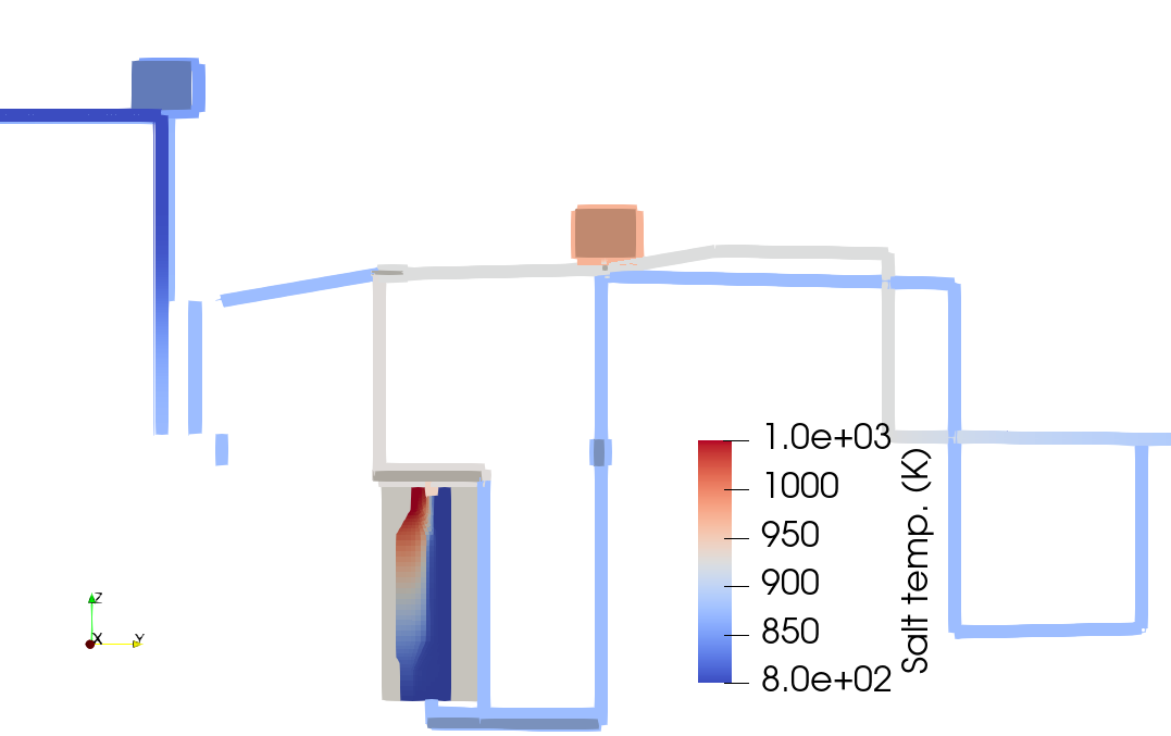
Salt temperature through the Mk1-FHR plant model
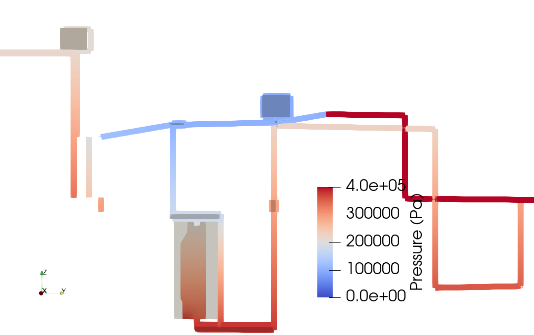
Pressure through the Mk1-FHR plant model
Acknowledgements
The model was created with support from Daniel Nunez at ANL and Cole Mueller at INL.
References
No citations exist within this document.(pbfhr/mark1/plant/ss1_combined.i)
# ==============================================================================
# Model description
# Application : Pronghorn
# ------------------------------------------------------------------------------
# Idaho Falls, INL, August 10, 2020
# Author(s): Dr. Guillaume Giudicelli, Dr. Paolo Balestra, Dr. April Novak
# If using or referring to this model, please cite as explained in
# https://mooseframework.inl.gov/virtual_test_bed/citing.html
# ------------------------------------------------------------------------------
#
# NOTE: This model is deprecated and is scheduled for removal from the VTB
#
# ==============================================================================
# - Coupled fluid-solid thermal hydraulics model of the Mk1-FHR
# ==============================================================================
# - The Model has been built based on [1-2].
# ------------------------------------------------------------------------------
# [1] Multiscale Core Thermal Hydraulics Analysis of the Pebble Bed Fluoride
#     Salt Cooled High Temperature Reactor (PB-FHR), A. Novak et al.
# [2] Technical Description of the “Mark 1” Pebble-Bed Fluoride-Salt-Cooled
#     High-Temperature Reactor (PB-FHR) Power Plant, UC Berkeley report 14-002
# [3] Molten salts database for energy applications, Serrano-Lopez et al.
#     https://arxiv.org/pdf/1307.7343.pdf
# [4] Heat Transfer Salts for Nuclear Reactor Systems - chemistry control,
#     corrosion mitigation and modeling, CFP-10-100, Anderson et al.
#     https://neup.inl.gov/SiteAssets/Final%20%20Reports/FY%202010/
#     10-905%20NEUP%20Final%20Report.pdf
# ==============================================================================
# MODEL PARAMETERS
# ==============================================================================
# Problem Parameters -----------------------------------------------------------

blocks_pebbles = '3 4'
blocks_fluid = '3 4 5 6'
blocks_solid = '1 2 6 7 8 9 10'

# Material compositions
UO2_phase_fraction = 1.20427291e-01
buffer_phase_fraction = 2.86014816e-01
ipyc_phase_fraction = 1.59496539e-01
sic_phase_fraction = 1.96561801e-01
opyc_phase_fraction = 2.37499553e-01
TRISO_phase_fraction = 3.09266232e-01
core_phase_fraction = 5.12000000e-01
fuel_matrix_phase_fraction = 3.01037037e-01
shell_phase_fraction = 1.86962963e-01

# FLiBe properties #TODO: Rely only on PronghornFluidProps
fluid_mu = 7.5e-3 # Pa.s at 900K [3]
# k_fluid =  1.1     # suggested constant [3]
# cp_fluid = 2385    # suggested constant [3]
rho_fluid = 1970.0 # kg/m3 at 900K [3]
alpha_b = 2e-4 # /K from [4]

# Graphite properties
heat_capacity_multiplier = 1e0 # >1 gets faster to steady state
solid_rho = 1780.0
# solid_k = 26.0
solid_cp = '${fparse 1697.0*heat_capacity_multiplier}'

# Core geometry
pebble_diameter = 0.03
bed_porosity = 0.4
IR_porosity = 0
OR_porosity = 0.1123
plenum_porosity = 0.5
model_inlet_rin = 0.45
model_inlet_rout = 0.8574
# model_vol        = 10.4
model_inlet_area = '${fparse 3.14159265 * (model_inlet_rout * model_inlet_rout - model_inlet_rin * model_inlet_rin)}'

# The convention for friction factors changed
darcy_conversion_plenum = '${fparse rho_fluid / plenum_porosity / fluid_mu}'
# The porosity simplfies out from the previous definition of the coefficients
darcy_conversion_or = '${fparse rho_fluid / fluid_mu}'
forchheimer_partial_conversion = 2 # divide further by speed

# Outer reflector drag parameters
# TODO: tune using CFD
# TODO: verify current values (imported from [1])
Ah = '${fparse 1337.76 * darcy_conversion_or}'
Bh = '${fparse 2.58 * forchheimer_partial_conversion}'
Av = '${fparse 599.30 * darcy_conversion_or}'
Bv = '${fparse 0.95 * forchheimer_partial_conversion}'
Dh = 0.02582
Dv = 0.02006

# Plenum drag parameters. The core hot legs cannot be represented in 2D RZ
# accurately, so this should be tuned to obtain the desired mass flow rates
plenum_friction = '${fparse 0.5 * darcy_conversion_plenum}'

# Operating parameters
# mfr = 976.0            # kg/s, from [2]
# total_power = 236.0e6  # W, from [2]
inlet_T_fluid = 873.15 # K, from [2]
# inlet_vel_y_ini = ${fparse mfr / model_inlet_area / rho_fluid} # superficial
# power_density = ${fparse total_power / model_vol / 258 * 236}  # adjusted using power pp
# outlet_pressure_val = 2e5

# ==============================================================================
# GEOMETRY AND MESH
# ==============================================================================

[Mesh]
  coord_type = RZ
  # Mesh should be fairly orthogonal for finite volume fluid flow
  # If you are running this input file for the first time, run core_with_reflectors.py
  # in pbfhr/steady/meshes using Cubit to generate the mesh
  # Modify the parameters (mesh size, refinement areas) for each application
  # neutronics, thermal hydraulics and fuel performance
  uniform_refine = 1
  [fmg]
    type = FileMeshGenerator
    file = '../steady/meshes/core_pronghorn.e'
  []
  [barrel]
    type = SideSetsBetweenSubdomainsGenerator
    primary_block = 6
    paired_block = 7
    input = fmg
    new_boundary = 'barrel_wall'
  []
  [OR_inlet]
    type = ParsedGenerateSideset
    combinatorial_geometry = 'abs(y) < 1e-10'
    new_sideset_name = 'OR_horizontal_bottom'
    included_subdomains = '6'
    input = barrel
  []
  [OR_outlet]
    type = ParsedGenerateSideset
    combinatorial_geometry = 'abs(y - 5.3125) < 1e-10'
    new_sideset_name = 'OR_horizontal_top'
    included_subdomains = '6'
    input = OR_inlet
  []
  [add_bed_right]
    type = SideSetsBetweenSubdomainsGenerator
    input = OR_outlet
    new_boundary = 'bed_right'
    primary_block = '6'
    paired_block = '4 5'
  []
  [remove_bad_sideset]
    type = BoundaryDeletionGenerator
    input = add_bed_right
    boundary_names = bed_left
  []
  [add_sideset_again]
    type = SideSetsBetweenSubdomainsGenerator
    input = remove_bad_sideset
    new_boundary = 'bed_left'
    primary_block = '3'
    paired_block = '1 2'
  []
[]

[Problem]
  # We use a restart file to heat up the reflector beforehand, to get SAM and Pgh in agreement
  restart_file_base = ss1_combined_initial_checkpoint_cp/LATEST
  force_restart = true
[]

[GlobalParams]
  rho = 'rho'
  porosity = porosity_viz
  characteristic_length = 0.03
  pebble_diameter = ${pebble_diameter}
  speed = 'speed'

  fp = fp
  T_solid = T_solid
  T_fluid = T_fluid
  pressure = pressure

  vel_x = 'superficial_vel_x'
  vel_y = 'superficial_vel_y'

  fv = true
  rhie_chow_user_object = 'pins_rhie_chow_interpolator'
[]

# ==============================================================================
# VARIABLES AND KERNELS
# ==============================================================================

[Problem]
  kernel_coverage_check = false
[]

[Modules]
  [NavierStokesFV]
    # General parameters
    compressibility = 'incompressible'
    porous_medium_treatment = true
    add_energy_equation = true
    boussinesq_approximation = true
    block = ${blocks_fluid}

    # Variables
    velocity_variable = 'superficial_vel_x superficial_vel_y'
    pressure_variable = 'pressure'
    fluid_temperature_variable = 'T_fluid'

    # Material properties
    density = ${rho_fluid}
    dynamic_viscosity = 'mu'
    thermal_conductivity = 'kappa'
    specific_heat = 'cp'
    thermal_expansion = 'alpha_b'
    porosity = 'porosity'

    # Boussinesq parameters
    gravity = '0 -9.81 0'
    ref_temperature = ${inlet_T_fluid}

    # Wall boundary conditions
    wall_boundaries = 'bed_left barrel_wall'
    momentum_wall_types = 'slip slip'
    energy_wall_types = 'heatflux heatflux'
    energy_wall_function = '0 0'

    # Inlet boundary conditions
    inlet_boundaries = 'bed_horizontal_bottom OR_horizontal_bottom'
    momentum_inlet_types = 'fixed-velocity fixed-velocity'
    momentum_inlet_function = '0 inlet_vel_y_fun; 0 0'
    energy_inlet_types = 'fixed-temperature heatflux'
    energy_inlet_function = 'T_inlet_fun 0'
    # so the flux BCs have to be used consistently across all equations

    # Outlet boundary conditions
    outlet_boundaries = 'bed_horizontal_top plenum_top OR_horizontal_top'
    momentum_outlet_types = 'fixed-pressure fixed-pressure fixed-pressure'
    pressure_function = 'pressure_out_fun pressure_out_fun pressure_out_fun'

    # Porous flow parameters
    ambient_convection_blocks = ${blocks_pebbles}
    ambient_convection_alpha = 'alpha'
    ambient_temperature = 'T_solid'

    # Friction in porous media
    friction_types = 'darcy forchheimer'
    friction_coeffs = 'Darcy_coefficient Forchheimer_coefficient'

    # Numerical scheme
    momentum_advection_interpolation = 'upwind'
    mass_advection_interpolation = 'upwind'
    energy_advection_interpolation = 'upwind'
  []
[]

[Variables]
  [superficial_vel_x]
    type = PINSFVSuperficialVelocityVariable
    block = ${blocks_fluid}
  []
  [superficial_vel_y]
    type = PINSFVSuperficialVelocityVariable
    block = ${blocks_fluid}
  []
  [pressure]
    type = INSFVPressureVariable
    block = ${blocks_fluid}
  []
  [T_fluid]
    type = INSFVEnergyVariable
    block = ${blocks_fluid}
  []
  [T_solid]
    type = INSFVEnergyVariable
  []
[]

[FVKernels]
  # Solid Energy equation.
  [temp_solid_time_core]
    type = PINSFVEnergyTimeDerivative
    variable = T_solid
    cp = 'cp_s'
    rho = ${solid_rho}
    is_solid = true
    block = ${blocks_fluid}
  []
  [temp_solid_time]
    type = PINSFVEnergyTimeDerivative
    variable = T_solid
    cp = 'cp_s'
    rho = 'rho_s'
    porosity = 0
    is_solid = true
    block = ${blocks_solid}
  []
  [temp_solid_conduction_core]
    type = FVDiffusion
    variable = T_solid
    coeff = 'kappa_s'
    block = ${blocks_fluid}
    # For backwards compatibility of testing. Please use harmonic (default)
    coeff_interp_method = 'average'
  []
  [temp_solid_conduction]
    type = FVDiffusion
    variable = T_solid
    coeff = 'k_s'
    block = ${blocks_solid}
    # For backwards compatibility of testing. Please use harmonic (default)
    coeff_interp_method = 'average'
  []
  [temp_solid_source]
    type = FVCoupledForce
    variable = T_solid
    v = power_distribution
    block = '3'
  []
  [temp_fluid_to_solid]
    type = PINSFVEnergyAmbientConvection
    variable = T_solid
    is_solid = true
    h_solid_fluid = 'alpha'
    block = ${blocks_fluid}
  []
[]

[FVInterfaceKernels]
  [diffusion_interface]
    type = FVDiffusionInterface
    boundary = 'bed_left'
    subdomain1 = '3 4 5'
    subdomain2 = '1 2 6'
    coeff1 = 'kappa_s'
    coeff2 = 'k_s'
    variable1 = 'T_solid'
    variable2 = 'T_solid'
    # For backwards compatibility of testing. Please use harmonic (default)
    coeff_interp_method = 'average'
  []
[]

# ==============================================================================
# AUXVARIABLES AND AUXKERNELS
# ==============================================================================
[AuxVariables]
  [power_distribution]
    type = MooseVariableFVReal
    block = '3'
  []
  [porosity_viz]
    type = MooseVariableFVReal
    block = ${blocks_fluid}
  []
[]

[AuxKernels]
  [eps]
    type = FunctorAux
    variable = porosity_viz
    functor = porosity
    block = ${blocks_fluid}
    execute_on = 'INITIAL'
  []
[]

# ==============================================================================
# INITIAL CONDITIONS AND FUNCTIONS
# ==============================================================================
[ICs]
  # No need for initial conditions for a restart simulation
[]

[Functions]
  # Convert postprocessor inputs to functions
  [inlet_vel_y_fun]
    type = ParsedFunction
    expression = 'inlet_vel_y_pp'
    symbol_names = 'inlet_vel_y_pp'
    symbol_values = 'inlet_vel_y_pp'
  []
  [pressure_out_fun]
    type = ParsedFunction
    expression = 'outlet_pressure'
    symbol_names = 'outlet_pressure'
    symbol_values = 'outlet_pressure'
  []
  [T_inlet_fun]
    type = ParsedFunction
    expression = 'inlet_temp_fluid'
    symbol_names = 'inlet_temp_fluid'
    symbol_values = 'inlet_temp_fluid'
  []
[]

# ==============================================================================
# BOUNDARY CONDITIONS
# ==============================================================================
[FVBCs]
  [outer]
    type = FVDirichletBC
    variable = T_solid
    boundary = 'brick_surface'
    value = '${fparse 35 + 273.15}'
  []
[]

# ==============================================================================
# FLUID PROPERTIES, MATERIALS AND USER OBJECTS
# ==============================================================================
[FluidProperties]
  [fp]
    type = FlibeFluidProperties
  []
[]

[FunctorMaterials]
  # solid material properties
  [solid_fuel_pebbles]
    type = PronghornSolidFunctorMaterialPT
    solid = pebble
    block = '3'
  []
  [solid_blanket_pebbles]
    type = PronghornSolidFunctorMaterialPT
    solid = graphite
    block = '4'
  []
  [plenum_and_OR]
    type = PronghornSolidFunctorMaterialPT
    solid = graphite
    block = '5 6 8'
  []
  [IR]
    type = PronghornSolidFunctorMaterialPT
    solid = inner_reflector
    block = '1 2'
  []
  [barrel_and_vessel]
    type = PronghornSolidFunctorMaterialPT
    solid = stainless_steel
    block = '7 9'
  []
  [firebrick_properties]
    type = ADGenericFunctorMaterial
    prop_names = 'rho_s         cp_s        k_s'
    prop_values = '${solid_rho} ${solid_cp} 0.26'
    block = '10'
  []

  # FLUID
  [alpha_boussinesq]
    type = ADGenericFunctorMaterial
    prop_names = 'alpha_b rho'
    prop_values = '${alpha_b} ${rho_fluid}'
    block = ${blocks_fluid}
    define_dot_functors = false
  []
  [fluidprops]
    type = GeneralFunctorFluidProps
    block = ${blocks_fluid}
    mu_rampdown = 1
  []

  # closures in the pebble bed
  [alpha]
    type = FunctorWakaoPebbleBedHTC
    block = ${blocks_pebbles}
  []
  [drag]
    type = FunctorKTADragCoefficients
    block = ${blocks_pebbles}
  []
  [kappa]
    type = FunctorLinearPecletKappaFluid
    block = ${blocks_pebbles}
  []
  [kappa_s]
    type = FunctorPebbleBedKappaSolid
    emissivity = 0.8
    Youngs_modulus = 9e9
    Poisson_ratio = 0.136
    wall_distance = wall_dist
    block = ${blocks_pebbles}
    T_solid = T_solid
    acceleration = '0 -9.81 0'
  []

  # closures in the outer reflector and the plenum
  [Fh]
    type = ADParsedFunctorMaterial
    property_name = Fh
    expression = 'Bh / Dh / speed'
    functor_symbols = 'Bh Dh speed'
    functor_names = '${Bh} ${Dh} speed'
  []
  [Fv]
    type = ADParsedFunctorMaterial
    property_name = Fv
    expression = 'Bv / Dv / speed'
    functor_symbols = 'Bv Dv speed'
    functor_names = '${Bv} ${Dv} speed'
  []
  [drag_OR]
    type = FunctorAnisotropicFunctorDragCoefficients
    Darcy_coefficient = '${fparse Ah / Dh / Dh} ${fparse Av / Dv / Dv} ${fparse Av / Dv / Dv}'
    Forchheimer_coefficient = 'Fh Fv Fv'
    block = '6'
  []
  [drag_plenum]
    type = ADGenericVectorFunctorMaterial
    prop_names = 'Darcy_coefficient Forchheimer_coefficient'
    prop_values = '${plenum_friction} ${plenum_friction} ${plenum_friction}
                   0 0 0'
    block = '5'
  []
  [alpha_OR_plenum]
    type = ADGenericFunctorMaterial
    prop_names = 'alpha'
    prop_values = '0.0'
    block = '5 6'
  []
  [kappa_OR_plenum]
    type = FunctorKappaFluid
    block = '5 6'
  []
  [kappa_s_OR_plenum]
    type = FunctorVolumeAverageKappaSolid
    block = '5 6'
  []

  # porosity
  [porosity]
    type = ADPiecewiseByBlockFunctorMaterial
    prop_name = 'porosity'
    subdomain_to_prop_value = '3 ${bed_porosity}
                               4 ${bed_porosity}
                               5 ${plenum_porosity}
                               6 ${OR_porosity}
                               7 ${OR_porosity}' # !!!
  []
[]

[UserObjects]
  [graphite]
    type = FunctionSolidProperties
    rho_s = 1780
    cp_s = '${fparse 1800.0 * heat_capacity_multiplier}'
    k_s = 26.0
  []
  [pebble_graphite]
    type = FunctionSolidProperties
    rho_s = 1600.0
    cp_s = 1800.0
    k_s = 15.0
  []
  [pebble_core]
    type = FunctionSolidProperties
    rho_s = 1450.0
    cp_s = 1800.0
    k_s = 15.0
  []
  [UO2]
    type = FunctionSolidProperties
    rho_s = 11000.0
    cp_s = 400.0
    k_s = 3.5
  []
  [pyc]
    type = PyroliticGraphite # (constant)
  []
  [buffer]
    type = PorousGraphite # (constant)
  []
  [SiC]
    type = FunctionSolidProperties
    rho_s = 3180.0
    cp_s = 1300.0
    k_s = 13.9
  []
  [TRISO]
    type = CompositeSolidProperties
    materials = 'UO2 buffer pyc SiC pyc'
    fractions = '${UO2_phase_fraction} ${buffer_phase_fraction} ${ipyc_phase_fraction} ${sic_phase_fraction} ${opyc_phase_fraction}'
  []
  [fuel_matrix]
    type = CompositeSolidProperties
    materials = 'TRISO pebble_graphite'
    fractions = '${TRISO_phase_fraction} ${fparse 1.0 - TRISO_phase_fraction}'
    k_mixing = 'chiew'
  []
  [pebble]
    type = CompositeSolidProperties
    materials = 'pebble_core fuel_matrix pebble_graphite'
    fractions = '${core_phase_fraction} ${fuel_matrix_phase_fraction} ${shell_phase_fraction}'
  []
  [stainless_steel]
    type = StainlessSteel
  []
  [solid_flibe]
    type = FunctionSolidProperties
    rho_s = 1986.62668
    cp_s = 2416.0
    k_s = 1.0665
  []
  [inner_reflector]
    type = CompositeSolidProperties
    materials = 'solid_flibe graphite'
    fractions = '${IR_porosity} ${fparse 1.0 - IR_porosity}'
  []
  [wall_dist]
    type = WallDistanceAngledCylindricalBed
    outer_radius_x = '0.8574 0.8574 1.25 1.25 0.89 0.89'
    outer_radius_y = '0.0 0.709 1.389 3.889 4.5125 5.3125'
    inner_radius_x = '0.45 0.45 0.35 0.35 0.71 0.71'
    inner_radius_y = '0.0 0.859 1.0322 3.889 4.5125 5.3125'
  []
[]

# ==============================================================================
# EXECUTION PARAMETERS
# ==============================================================================
[Executioner]
  type = Transient

  solve_type = 'NEWTON'
  petsc_options_iname = '-pc_type -sub_pc_type -sub_pc_factor_shift_type -ksp_gmres_restart'
  petsc_options_value = 'asm      lu           NONZERO                   200'
  line_search = 'none'

  # Iterations parameters
  l_max_its = 500
  l_tol = 1e-8
  nl_max_its = 25
  nl_rel_tol = 5e-7
  nl_abs_tol = 5e-7

  # Automatic scaling
  automatic_scaling = true

  # Problem time parameters
  dtmin = 0.1
  dtmax = 2e4

  # To run a 100s transient
  start_time = 0
  end_time = 100

  [TimeStepper]
    type = IterationAdaptiveDT
    dt = 1
    cutback_factor = 0.5
    growth_factor = 2.0
  []

  # Time integration scheme
  scheme = 'implicit-euler'

  # Fixed point iterations with SAM
  fixed_point_max_its = 10
  fixed_point_abs_tol = 1e-5
  accept_on_max_fixed_point_iteration = true

  # Steady state detection.
  steady_state_detection = true
  steady_state_tolerance = 1e-8
  steady_state_start_time = 200000
[]

# ==============================================================================
# MULTIAPPS FOR PEBBLE MODEL AND PRIMARY LOOP
# ==============================================================================
[MultiApps]
  [pebble_mesh]
    type = TransientMultiApp
    execute_on = 'FINAL'
    # This must be set so that the default SAM executioner parameters are used
    app_type = 'SamApp'
    input_files = 'ss3_coarse_pebble_mesh.i'
    cli_args = 'Outputs/console=false'
  []

  [primary]
    type = TransientMultiApp
    app_type = 'SamApp'
    input_files = ss2_primary.i
    max_procs_per_app = 1
    execute_on = 'timestep_end'

    # Parameters if Pronghorn takes larger steps than SAM
    # sub_cycling = true
    # print_sub_cycles = false

    # Parameters if Pronghorn and SAM steps match
    # catch_up = true
    # keep_solution_during_restore = true
  []
[]

[Transfers]
  # Pebble simulations
  [fuel_matrix_heat_source]
    type = MultiAppProjectionTransfer
    to_multi_app = pebble_mesh
    source_variable = power_distribution
    variable = power_distribution
  []
  [pebble_surface_temp]
    type = MultiAppProjectionTransfer
    to_multi_app = pebble_mesh
    source_variable = T_solid
    variable = temp_solid
  []

  # Primary and secondary loops
  [send_flow_BCs]
    type = MultiAppPostprocessorVectorTransfer
    to_multi_app = primary
    from_postprocessors = 'pressure_in mass_flow_out T_flow_out T_flow_in'
    to_postprocessors = 'Core_inlet_pressure Core_outlet_mdot Core_outlet_T Core_inlet_T_reversal'
  []
  [receive_flow_BCs]
    type = MultiAppPostprocessorVectorTransfer
    from_multi_app = primary
    from_postprocessors = 'Core_outlet_p Core_inlet_mdot Core_inlet_T'
    to_postprocessors = 'outlet_pressure inlet_mdot inlet_temp_fluid'
    # Initial execution is important to avoid using a default BC
    execute_on = 'INITIAL TIMESTEP_END'
  []
[]

# ==============================================================================
# POSTPROCESSORS DEBUG AND OUTPUTS
# ==============================================================================
[Postprocessors]
  # Received from SAM for primary loop coupling
  [inlet_mdot]
    type = Receiver
    default = 9.784508e+02 #${mfr}
    execute_on = 'INITIAL TIMESTEP_END TRANSFER'
  []
  [inlet_vel_y_pp]
    type = ParsedPostprocessor
    function = 'inlet_mdot / model_inlet_area / rho_fluid'
    pp_names = 'inlet_mdot'
    constant_names = 'model_inlet_area rho_fluid'
    constant_expressions = '${model_inlet_area} ${rho_fluid}'
    execute_on = 'INITIAL TIMESTEP_END TRANSFER'
  []
  [inlet_temp_fluid]
    type = Receiver
    default = 8.741515e+02 #${inlet_T_fluid}
    execute_on = 'INITIAL TIMESTEP_END TRANSFER'
  []
  [outlet_pressure]
    type = Receiver
    default = 1.865956e+05 #${outlet_pressure_val}
    execute_on = 'INITIAL TIMESTEP_END TRANSFER'
  []

  # Transfered to SAM for primary loop coupling
  [pressure_in]
    type = SideAverageValue
    boundary = 'bed_horizontal_bottom'
    variable = pressure
    execute_on = 'INITIAL TIMESTEP_END TRANSFER'
  []
  [mass_flow_out]
    type = VolumetricFlowRate
    boundary = 'bed_horizontal_top plenum_top OR_horizontal_top'
    advected_quantity = ${rho_fluid}
    execute_on = 'INITIAL TIMESTEP_END TRANSFER'
  []
  [T_flow_in]
    type = ParsedPostprocessor
    function = '-e_flow_in_m / inlet_mdot / cp_fluid'
    pp_names = 'e_flow_in_m inlet_mdot'
    constant_names = 'cp_fluid'
    constant_expressions = '2416'
    execute_on = 'INITIAL TIMESTEP_END TRANSFER'
  []
  [T_flow_out]
    type = ParsedPostprocessor
    function = 'e_flow_out / mass_flow_out / cp_fluid'
    pp_names = 'e_flow_out mass_flow_out'
    constant_names = 'cp_fluid'
    constant_expressions = '2416'
    execute_on = 'INITIAL TIMESTEP_END TRANSFER'
  []

  # Solution Analysis
  [max_Tf]
    type = ElementExtremeValue
    variable = T_fluid
    block = ${blocks_fluid}
  []
  [max_vy]
    type = ElementExtremeValue
    variable = superficial_vel_y
    block = ${blocks_fluid}
  []
  [power]
    type = ElementIntegralVariablePostprocessor
    variable = power_distribution
    block = '3'
    execute_on = 'INITIAL TIMESTEP_BEGIN TRANSFER TIMESTEP_END'
  []
  [pressure_drop]
    type = DifferencePostprocessor
    value1 = outlet_pressure
    value2 = pressure_in
  []

  # Energy balance
  # Energy balance will be shown once #18119 #18123 are merged in MOOSE
  # [outer_heat_loss]
  #   type = ADSideDiffusiveFluxIntegral
  #   boundary = 'brick_surface'
  #   variable = T_solid
  #   diffusivity = 'k_s'
  #   execute_on = 'INITIAL TIMESTEP_END'
  # []
  [e_flow_in_m]
    type = VolumetricFlowRate
    boundary = 'bed_horizontal_bottom OR_horizontal_bottom'
    advected_quantity = 'rho_cp_temp'
  []
  # [diffusion_in]
  #   type = ADSideVectorDiffusivityFluxIntegral
  #   variable = T_fluid
  #   boundary = 'bed_horizontal_bottom OR_horizontal_bottom'
  #   diffusivity = 'kappa'
  # []
  # diffusion at the top is 0 because of the fully developped flow assumption
  [e_flow_out]
    type = VolumetricFlowRate
    boundary = 'bed_horizontal_top plenum_top OR_horizontal_top'
    advected_quantity = 'rho_cp_temp'
  []
  [core_balance]
    type = ParsedPostprocessor
    pp_names = 'power e_flow_in_m e_flow_out' #diffusion_in  outer_heat_loss'
    function = 'power - e_flow_in_m - e_flow_out' # + diffusion_in + outer_heat_loss'
  []

  # Bypass
  [mass_flow_OR]
    type = VolumetricFlowRate
    boundary = 'OR_horizontal_top'
    advected_quantity = 'rho'
    execute_on = 'INITIAL TIMESTEP_END'
  []
  [mass_flow_plenum]
    type = VolumetricFlowRate
    boundary = 'plenum_top'
    advected_quantity = 'rho'
    execute_on = 'INITIAL TIMESTEP_END'
  []
  [bypass_fraction]
    type = ParsedPostprocessor
    pp_names = 'mass_flow_OR mass_flow_out'
    function = 'mass_flow_OR / mass_flow_out'
  []
  [plenum_fraction]
    type = ParsedPostprocessor
    pp_names = 'mass_flow_plenum mass_flow_out'
    function = 'mass_flow_plenum / mass_flow_out'
  []

  # Miscellaneous
  [h]
    type = AverageElementSize
    outputs = 'console csv'
    execute_on = 'timestep_end'
  []
  [coupling_its_primary]
    type = NumFixedPointIterations
  []
  [num_fixed_point]
    type = Receiver
    default = 0
  []
[]

[Outputs]
  csv = true
  [console]
    type = Console
    show = 'T_flow_in inlet_temp_fluid T_flow_out pressure_in outlet_pressure inlet_mdot mass_flow_out'
  []
  [exodus]
    type = Exodus
  []
  [checkpoint]
    type = Checkpoint
    num_files = 2
  []
  # Reduce base output
  print_linear_converged_reason = false
  print_linear_residuals = false
  print_nonlinear_converged_reason = false
[]
(pbfhr/mark1/plant/ss1_combined.i)
# ==============================================================================
# Model description
# Application : Pronghorn
# ------------------------------------------------------------------------------
# Idaho Falls, INL, August 10, 2020
# Author(s): Dr. Guillaume Giudicelli, Dr. Paolo Balestra, Dr. April Novak
# If using or referring to this model, please cite as explained in
# https://mooseframework.inl.gov/virtual_test_bed/citing.html
# ------------------------------------------------------------------------------
#
# NOTE: This model is deprecated and is scheduled for removal from the VTB
#
# ==============================================================================
# - Coupled fluid-solid thermal hydraulics model of the Mk1-FHR
# ==============================================================================
# - The Model has been built based on [1-2].
# ------------------------------------------------------------------------------
# [1] Multiscale Core Thermal Hydraulics Analysis of the Pebble Bed Fluoride
#     Salt Cooled High Temperature Reactor (PB-FHR), A. Novak et al.
# [2] Technical Description of the “Mark 1” Pebble-Bed Fluoride-Salt-Cooled
#     High-Temperature Reactor (PB-FHR) Power Plant, UC Berkeley report 14-002
# [3] Molten salts database for energy applications, Serrano-Lopez et al.
#     https://arxiv.org/pdf/1307.7343.pdf
# [4] Heat Transfer Salts for Nuclear Reactor Systems - chemistry control,
#     corrosion mitigation and modeling, CFP-10-100, Anderson et al.
#     https://neup.inl.gov/SiteAssets/Final%20%20Reports/FY%202010/
#     10-905%20NEUP%20Final%20Report.pdf
# ==============================================================================
# MODEL PARAMETERS
# ==============================================================================
# Problem Parameters -----------------------------------------------------------

blocks_pebbles = '3 4'
blocks_fluid = '3 4 5 6'
blocks_solid = '1 2 6 7 8 9 10'

# Material compositions
UO2_phase_fraction = 1.20427291e-01
buffer_phase_fraction = 2.86014816e-01
ipyc_phase_fraction = 1.59496539e-01
sic_phase_fraction = 1.96561801e-01
opyc_phase_fraction = 2.37499553e-01
TRISO_phase_fraction = 3.09266232e-01
core_phase_fraction = 5.12000000e-01
fuel_matrix_phase_fraction = 3.01037037e-01
shell_phase_fraction = 1.86962963e-01

# FLiBe properties #TODO: Rely only on PronghornFluidProps
fluid_mu = 7.5e-3 # Pa.s at 900K [3]
# k_fluid =  1.1     # suggested constant [3]
# cp_fluid = 2385    # suggested constant [3]
rho_fluid = 1970.0 # kg/m3 at 900K [3]
alpha_b = 2e-4 # /K from [4]

# Graphite properties
heat_capacity_multiplier = 1e0 # >1 gets faster to steady state
solid_rho = 1780.0
# solid_k = 26.0
solid_cp = '${fparse 1697.0*heat_capacity_multiplier}'

# Core geometry
pebble_diameter = 0.03
bed_porosity = 0.4
IR_porosity = 0
OR_porosity = 0.1123
plenum_porosity = 0.5
model_inlet_rin = 0.45
model_inlet_rout = 0.8574
# model_vol        = 10.4
model_inlet_area = '${fparse 3.14159265 * (model_inlet_rout * model_inlet_rout - model_inlet_rin * model_inlet_rin)}'

# The convention for friction factors changed
darcy_conversion_plenum = '${fparse rho_fluid / plenum_porosity / fluid_mu}'
# The porosity simplfies out from the previous definition of the coefficients
darcy_conversion_or = '${fparse rho_fluid / fluid_mu}'
forchheimer_partial_conversion = 2 # divide further by speed

# Outer reflector drag parameters
# TODO: tune using CFD
# TODO: verify current values (imported from [1])
Ah = '${fparse 1337.76 * darcy_conversion_or}'
Bh = '${fparse 2.58 * forchheimer_partial_conversion}'
Av = '${fparse 599.30 * darcy_conversion_or}'
Bv = '${fparse 0.95 * forchheimer_partial_conversion}'
Dh = 0.02582
Dv = 0.02006

# Plenum drag parameters. The core hot legs cannot be represented in 2D RZ
# accurately, so this should be tuned to obtain the desired mass flow rates
plenum_friction = '${fparse 0.5 * darcy_conversion_plenum}'

# Operating parameters
# mfr = 976.0            # kg/s, from [2]
# total_power = 236.0e6  # W, from [2]
inlet_T_fluid = 873.15 # K, from [2]
# inlet_vel_y_ini = ${fparse mfr / model_inlet_area / rho_fluid} # superficial
# power_density = ${fparse total_power / model_vol / 258 * 236}  # adjusted using power pp
# outlet_pressure_val = 2e5

# ==============================================================================
# GEOMETRY AND MESH
# ==============================================================================

[Mesh]
  coord_type = RZ
  # Mesh should be fairly orthogonal for finite volume fluid flow
  # If you are running this input file for the first time, run core_with_reflectors.py
  # in pbfhr/steady/meshes using Cubit to generate the mesh
  # Modify the parameters (mesh size, refinement areas) for each application
  # neutronics, thermal hydraulics and fuel performance
  uniform_refine = 1
  [fmg]
    type = FileMeshGenerator
    file = '../steady/meshes/core_pronghorn.e'
  []
  [barrel]
    type = SideSetsBetweenSubdomainsGenerator
    primary_block = 6
    paired_block = 7
    input = fmg
    new_boundary = 'barrel_wall'
  []
  [OR_inlet]
    type = ParsedGenerateSideset
    combinatorial_geometry = 'abs(y) < 1e-10'
    new_sideset_name = 'OR_horizontal_bottom'
    included_subdomains = '6'
    input = barrel
  []
  [OR_outlet]
    type = ParsedGenerateSideset
    combinatorial_geometry = 'abs(y - 5.3125) < 1e-10'
    new_sideset_name = 'OR_horizontal_top'
    included_subdomains = '6'
    input = OR_inlet
  []
  [add_bed_right]
    type = SideSetsBetweenSubdomainsGenerator
    input = OR_outlet
    new_boundary = 'bed_right'
    primary_block = '6'
    paired_block = '4 5'
  []
  [remove_bad_sideset]
    type = BoundaryDeletionGenerator
    input = add_bed_right
    boundary_names = bed_left
  []
  [add_sideset_again]
    type = SideSetsBetweenSubdomainsGenerator
    input = remove_bad_sideset
    new_boundary = 'bed_left'
    primary_block = '3'
    paired_block = '1 2'
  []
[]

[Problem]
  # We use a restart file to heat up the reflector beforehand, to get SAM and Pgh in agreement
  restart_file_base = ss1_combined_initial_checkpoint_cp/LATEST
  force_restart = true
[]

[GlobalParams]
  rho = 'rho'
  porosity = porosity_viz
  characteristic_length = 0.03
  pebble_diameter = ${pebble_diameter}
  speed = 'speed'

  fp = fp
  T_solid = T_solid
  T_fluid = T_fluid
  pressure = pressure

  vel_x = 'superficial_vel_x'
  vel_y = 'superficial_vel_y'

  fv = true
  rhie_chow_user_object = 'pins_rhie_chow_interpolator'
[]

# ==============================================================================
# VARIABLES AND KERNELS
# ==============================================================================

[Problem]
  kernel_coverage_check = false
[]

[Modules]
  [NavierStokesFV]
    # General parameters
    compressibility = 'incompressible'
    porous_medium_treatment = true
    add_energy_equation = true
    boussinesq_approximation = true
    block = ${blocks_fluid}

    # Variables
    velocity_variable = 'superficial_vel_x superficial_vel_y'
    pressure_variable = 'pressure'
    fluid_temperature_variable = 'T_fluid'

    # Material properties
    density = ${rho_fluid}
    dynamic_viscosity = 'mu'
    thermal_conductivity = 'kappa'
    specific_heat = 'cp'
    thermal_expansion = 'alpha_b'
    porosity = 'porosity'

    # Boussinesq parameters
    gravity = '0 -9.81 0'
    ref_temperature = ${inlet_T_fluid}

    # Wall boundary conditions
    wall_boundaries = 'bed_left barrel_wall'
    momentum_wall_types = 'slip slip'
    energy_wall_types = 'heatflux heatflux'
    energy_wall_function = '0 0'

    # Inlet boundary conditions
    inlet_boundaries = 'bed_horizontal_bottom OR_horizontal_bottom'
    momentum_inlet_types = 'fixed-velocity fixed-velocity'
    momentum_inlet_function = '0 inlet_vel_y_fun; 0 0'
    energy_inlet_types = 'fixed-temperature heatflux'
    energy_inlet_function = 'T_inlet_fun 0'
    # so the flux BCs have to be used consistently across all equations

    # Outlet boundary conditions
    outlet_boundaries = 'bed_horizontal_top plenum_top OR_horizontal_top'
    momentum_outlet_types = 'fixed-pressure fixed-pressure fixed-pressure'
    pressure_function = 'pressure_out_fun pressure_out_fun pressure_out_fun'

    # Porous flow parameters
    ambient_convection_blocks = ${blocks_pebbles}
    ambient_convection_alpha = 'alpha'
    ambient_temperature = 'T_solid'

    # Friction in porous media
    friction_types = 'darcy forchheimer'
    friction_coeffs = 'Darcy_coefficient Forchheimer_coefficient'

    # Numerical scheme
    momentum_advection_interpolation = 'upwind'
    mass_advection_interpolation = 'upwind'
    energy_advection_interpolation = 'upwind'
  []
[]

[Variables]
  [superficial_vel_x]
    type = PINSFVSuperficialVelocityVariable
    block = ${blocks_fluid}
  []
  [superficial_vel_y]
    type = PINSFVSuperficialVelocityVariable
    block = ${blocks_fluid}
  []
  [pressure]
    type = INSFVPressureVariable
    block = ${blocks_fluid}
  []
  [T_fluid]
    type = INSFVEnergyVariable
    block = ${blocks_fluid}
  []
  [T_solid]
    type = INSFVEnergyVariable
  []
[]

[FVKernels]
  # Solid Energy equation.
  [temp_solid_time_core]
    type = PINSFVEnergyTimeDerivative
    variable = T_solid
    cp = 'cp_s'
    rho = ${solid_rho}
    is_solid = true
    block = ${blocks_fluid}
  []
  [temp_solid_time]
    type = PINSFVEnergyTimeDerivative
    variable = T_solid
    cp = 'cp_s'
    rho = 'rho_s'
    porosity = 0
    is_solid = true
    block = ${blocks_solid}
  []
  [temp_solid_conduction_core]
    type = FVDiffusion
    variable = T_solid
    coeff = 'kappa_s'
    block = ${blocks_fluid}
    # For backwards compatibility of testing. Please use harmonic (default)
    coeff_interp_method = 'average'
  []
  [temp_solid_conduction]
    type = FVDiffusion
    variable = T_solid
    coeff = 'k_s'
    block = ${blocks_solid}
    # For backwards compatibility of testing. Please use harmonic (default)
    coeff_interp_method = 'average'
  []
  [temp_solid_source]
    type = FVCoupledForce
    variable = T_solid
    v = power_distribution
    block = '3'
  []
  [temp_fluid_to_solid]
    type = PINSFVEnergyAmbientConvection
    variable = T_solid
    is_solid = true
    h_solid_fluid = 'alpha'
    block = ${blocks_fluid}
  []
[]

[FVInterfaceKernels]
  [diffusion_interface]
    type = FVDiffusionInterface
    boundary = 'bed_left'
    subdomain1 = '3 4 5'
    subdomain2 = '1 2 6'
    coeff1 = 'kappa_s'
    coeff2 = 'k_s'
    variable1 = 'T_solid'
    variable2 = 'T_solid'
    # For backwards compatibility of testing. Please use harmonic (default)
    coeff_interp_method = 'average'
  []
[]

# ==============================================================================
# AUXVARIABLES AND AUXKERNELS
# ==============================================================================
[AuxVariables]
  [power_distribution]
    type = MooseVariableFVReal
    block = '3'
  []
  [porosity_viz]
    type = MooseVariableFVReal
    block = ${blocks_fluid}
  []
[]

[AuxKernels]
  [eps]
    type = FunctorAux
    variable = porosity_viz
    functor = porosity
    block = ${blocks_fluid}
    execute_on = 'INITIAL'
  []
[]

# ==============================================================================
# INITIAL CONDITIONS AND FUNCTIONS
# ==============================================================================
[ICs]
  # No need for initial conditions for a restart simulation
[]

[Functions]
  # Convert postprocessor inputs to functions
  [inlet_vel_y_fun]
    type = ParsedFunction
    expression = 'inlet_vel_y_pp'
    symbol_names = 'inlet_vel_y_pp'
    symbol_values = 'inlet_vel_y_pp'
  []
  [pressure_out_fun]
    type = ParsedFunction
    expression = 'outlet_pressure'
    symbol_names = 'outlet_pressure'
    symbol_values = 'outlet_pressure'
  []
  [T_inlet_fun]
    type = ParsedFunction
    expression = 'inlet_temp_fluid'
    symbol_names = 'inlet_temp_fluid'
    symbol_values = 'inlet_temp_fluid'
  []
[]

# ==============================================================================
# BOUNDARY CONDITIONS
# ==============================================================================
[FVBCs]
  [outer]
    type = FVDirichletBC
    variable = T_solid
    boundary = 'brick_surface'
    value = '${fparse 35 + 273.15}'
  []
[]

# ==============================================================================
# FLUID PROPERTIES, MATERIALS AND USER OBJECTS
# ==============================================================================
[FluidProperties]
  [fp]
    type = FlibeFluidProperties
  []
[]

[FunctorMaterials]
  # solid material properties
  [solid_fuel_pebbles]
    type = PronghornSolidFunctorMaterialPT
    solid = pebble
    block = '3'
  []
  [solid_blanket_pebbles]
    type = PronghornSolidFunctorMaterialPT
    solid = graphite
    block = '4'
  []
  [plenum_and_OR]
    type = PronghornSolidFunctorMaterialPT
    solid = graphite
    block = '5 6 8'
  []
  [IR]
    type = PronghornSolidFunctorMaterialPT
    solid = inner_reflector
    block = '1 2'
  []
  [barrel_and_vessel]
    type = PronghornSolidFunctorMaterialPT
    solid = stainless_steel
    block = '7 9'
  []
  [firebrick_properties]
    type = ADGenericFunctorMaterial
    prop_names = 'rho_s         cp_s        k_s'
    prop_values = '${solid_rho} ${solid_cp} 0.26'
    block = '10'
  []

  # FLUID
  [alpha_boussinesq]
    type = ADGenericFunctorMaterial
    prop_names = 'alpha_b rho'
    prop_values = '${alpha_b} ${rho_fluid}'
    block = ${blocks_fluid}
    define_dot_functors = false
  []
  [fluidprops]
    type = GeneralFunctorFluidProps
    block = ${blocks_fluid}
    mu_rampdown = 1
  []

  # closures in the pebble bed
  [alpha]
    type = FunctorWakaoPebbleBedHTC
    block = ${blocks_pebbles}
  []
  [drag]
    type = FunctorKTADragCoefficients
    block = ${blocks_pebbles}
  []
  [kappa]
    type = FunctorLinearPecletKappaFluid
    block = ${blocks_pebbles}
  []
  [kappa_s]
    type = FunctorPebbleBedKappaSolid
    emissivity = 0.8
    Youngs_modulus = 9e9
    Poisson_ratio = 0.136
    wall_distance = wall_dist
    block = ${blocks_pebbles}
    T_solid = T_solid
    acceleration = '0 -9.81 0'
  []

  # closures in the outer reflector and the plenum
  [Fh]
    type = ADParsedFunctorMaterial
    property_name = Fh
    expression = 'Bh / Dh / speed'
    functor_symbols = 'Bh Dh speed'
    functor_names = '${Bh} ${Dh} speed'
  []
  [Fv]
    type = ADParsedFunctorMaterial
    property_name = Fv
    expression = 'Bv / Dv / speed'
    functor_symbols = 'Bv Dv speed'
    functor_names = '${Bv} ${Dv} speed'
  []
  [drag_OR]
    type = FunctorAnisotropicFunctorDragCoefficients
    Darcy_coefficient = '${fparse Ah / Dh / Dh} ${fparse Av / Dv / Dv} ${fparse Av / Dv / Dv}'
    Forchheimer_coefficient = 'Fh Fv Fv'
    block = '6'
  []
  [drag_plenum]
    type = ADGenericVectorFunctorMaterial
    prop_names = 'Darcy_coefficient Forchheimer_coefficient'
    prop_values = '${plenum_friction} ${plenum_friction} ${plenum_friction}
                   0 0 0'
    block = '5'
  []
  [alpha_OR_plenum]
    type = ADGenericFunctorMaterial
    prop_names = 'alpha'
    prop_values = '0.0'
    block = '5 6'
  []
  [kappa_OR_plenum]
    type = FunctorKappaFluid
    block = '5 6'
  []
  [kappa_s_OR_plenum]
    type = FunctorVolumeAverageKappaSolid
    block = '5 6'
  []

  # porosity
  [porosity]
    type = ADPiecewiseByBlockFunctorMaterial
    prop_name = 'porosity'
    subdomain_to_prop_value = '3 ${bed_porosity}
                               4 ${bed_porosity}
                               5 ${plenum_porosity}
                               6 ${OR_porosity}
                               7 ${OR_porosity}' # !!!
  []
[]

[UserObjects]
  [graphite]
    type = FunctionSolidProperties
    rho_s = 1780
    cp_s = '${fparse 1800.0 * heat_capacity_multiplier}'
    k_s = 26.0
  []
  [pebble_graphite]
    type = FunctionSolidProperties
    rho_s = 1600.0
    cp_s = 1800.0
    k_s = 15.0
  []
  [pebble_core]
    type = FunctionSolidProperties
    rho_s = 1450.0
    cp_s = 1800.0
    k_s = 15.0
  []
  [UO2]
    type = FunctionSolidProperties
    rho_s = 11000.0
    cp_s = 400.0
    k_s = 3.5
  []
  [pyc]
    type = PyroliticGraphite # (constant)
  []
  [buffer]
    type = PorousGraphite # (constant)
  []
  [SiC]
    type = FunctionSolidProperties
    rho_s = 3180.0
    cp_s = 1300.0
    k_s = 13.9
  []
  [TRISO]
    type = CompositeSolidProperties
    materials = 'UO2 buffer pyc SiC pyc'
    fractions = '${UO2_phase_fraction} ${buffer_phase_fraction} ${ipyc_phase_fraction} ${sic_phase_fraction} ${opyc_phase_fraction}'
  []
  [fuel_matrix]
    type = CompositeSolidProperties
    materials = 'TRISO pebble_graphite'
    fractions = '${TRISO_phase_fraction} ${fparse 1.0 - TRISO_phase_fraction}'
    k_mixing = 'chiew'
  []
  [pebble]
    type = CompositeSolidProperties
    materials = 'pebble_core fuel_matrix pebble_graphite'
    fractions = '${core_phase_fraction} ${fuel_matrix_phase_fraction} ${shell_phase_fraction}'
  []
  [stainless_steel]
    type = StainlessSteel
  []
  [solid_flibe]
    type = FunctionSolidProperties
    rho_s = 1986.62668
    cp_s = 2416.0
    k_s = 1.0665
  []
  [inner_reflector]
    type = CompositeSolidProperties
    materials = 'solid_flibe graphite'
    fractions = '${IR_porosity} ${fparse 1.0 - IR_porosity}'
  []
  [wall_dist]
    type = WallDistanceAngledCylindricalBed
    outer_radius_x = '0.8574 0.8574 1.25 1.25 0.89 0.89'
    outer_radius_y = '0.0 0.709 1.389 3.889 4.5125 5.3125'
    inner_radius_x = '0.45 0.45 0.35 0.35 0.71 0.71'
    inner_radius_y = '0.0 0.859 1.0322 3.889 4.5125 5.3125'
  []
[]

# ==============================================================================
# EXECUTION PARAMETERS
# ==============================================================================
[Executioner]
  type = Transient

  solve_type = 'NEWTON'
  petsc_options_iname = '-pc_type -sub_pc_type -sub_pc_factor_shift_type -ksp_gmres_restart'
  petsc_options_value = 'asm      lu           NONZERO                   200'
  line_search = 'none'

  # Iterations parameters
  l_max_its = 500
  l_tol = 1e-8
  nl_max_its = 25
  nl_rel_tol = 5e-7
  nl_abs_tol = 5e-7

  # Automatic scaling
  automatic_scaling = true

  # Problem time parameters
  dtmin = 0.1
  dtmax = 2e4

  # To run a 100s transient
  start_time = 0
  end_time = 100

  [TimeStepper]
    type = IterationAdaptiveDT
    dt = 1
    cutback_factor = 0.5
    growth_factor = 2.0
  []

  # Time integration scheme
  scheme = 'implicit-euler'

  # Fixed point iterations with SAM
  fixed_point_max_its = 10
  fixed_point_abs_tol = 1e-5
  accept_on_max_fixed_point_iteration = true

  # Steady state detection.
  steady_state_detection = true
  steady_state_tolerance = 1e-8
  steady_state_start_time = 200000
[]

# ==============================================================================
# MULTIAPPS FOR PEBBLE MODEL AND PRIMARY LOOP
# ==============================================================================
[MultiApps]
  [pebble_mesh]
    type = TransientMultiApp
    execute_on = 'FINAL'
    # This must be set so that the default SAM executioner parameters are used
    app_type = 'SamApp'
    input_files = 'ss3_coarse_pebble_mesh.i'
    cli_args = 'Outputs/console=false'
  []

  [primary]
    type = TransientMultiApp
    app_type = 'SamApp'
    input_files = ss2_primary.i
    max_procs_per_app = 1
    execute_on = 'timestep_end'

    # Parameters if Pronghorn takes larger steps than SAM
    # sub_cycling = true
    # print_sub_cycles = false

    # Parameters if Pronghorn and SAM steps match
    # catch_up = true
    # keep_solution_during_restore = true
  []
[]

[Transfers]
  # Pebble simulations
  [fuel_matrix_heat_source]
    type = MultiAppProjectionTransfer
    to_multi_app = pebble_mesh
    source_variable = power_distribution
    variable = power_distribution
  []
  [pebble_surface_temp]
    type = MultiAppProjectionTransfer
    to_multi_app = pebble_mesh
    source_variable = T_solid
    variable = temp_solid
  []

  # Primary and secondary loops
  [send_flow_BCs]
    type = MultiAppPostprocessorVectorTransfer
    to_multi_app = primary
    from_postprocessors = 'pressure_in mass_flow_out T_flow_out T_flow_in'
    to_postprocessors = 'Core_inlet_pressure Core_outlet_mdot Core_outlet_T Core_inlet_T_reversal'
  []
  [receive_flow_BCs]
    type = MultiAppPostprocessorVectorTransfer
    from_multi_app = primary
    from_postprocessors = 'Core_outlet_p Core_inlet_mdot Core_inlet_T'
    to_postprocessors = 'outlet_pressure inlet_mdot inlet_temp_fluid'
    # Initial execution is important to avoid using a default BC
    execute_on = 'INITIAL TIMESTEP_END'
  []
[]

# ==============================================================================
# POSTPROCESSORS DEBUG AND OUTPUTS
# ==============================================================================
[Postprocessors]
  # Received from SAM for primary loop coupling
  [inlet_mdot]
    type = Receiver
    default = 9.784508e+02 #${mfr}
    execute_on = 'INITIAL TIMESTEP_END TRANSFER'
  []
  [inlet_vel_y_pp]
    type = ParsedPostprocessor
    function = 'inlet_mdot / model_inlet_area / rho_fluid'
    pp_names = 'inlet_mdot'
    constant_names = 'model_inlet_area rho_fluid'
    constant_expressions = '${model_inlet_area} ${rho_fluid}'
    execute_on = 'INITIAL TIMESTEP_END TRANSFER'
  []
  [inlet_temp_fluid]
    type = Receiver
    default = 8.741515e+02 #${inlet_T_fluid}
    execute_on = 'INITIAL TIMESTEP_END TRANSFER'
  []
  [outlet_pressure]
    type = Receiver
    default = 1.865956e+05 #${outlet_pressure_val}
    execute_on = 'INITIAL TIMESTEP_END TRANSFER'
  []

  # Transfered to SAM for primary loop coupling
  [pressure_in]
    type = SideAverageValue
    boundary = 'bed_horizontal_bottom'
    variable = pressure
    execute_on = 'INITIAL TIMESTEP_END TRANSFER'
  []
  [mass_flow_out]
    type = VolumetricFlowRate
    boundary = 'bed_horizontal_top plenum_top OR_horizontal_top'
    advected_quantity = ${rho_fluid}
    execute_on = 'INITIAL TIMESTEP_END TRANSFER'
  []
  [T_flow_in]
    type = ParsedPostprocessor
    function = '-e_flow_in_m / inlet_mdot / cp_fluid'
    pp_names = 'e_flow_in_m inlet_mdot'
    constant_names = 'cp_fluid'
    constant_expressions = '2416'
    execute_on = 'INITIAL TIMESTEP_END TRANSFER'
  []
  [T_flow_out]
    type = ParsedPostprocessor
    function = 'e_flow_out / mass_flow_out / cp_fluid'
    pp_names = 'e_flow_out mass_flow_out'
    constant_names = 'cp_fluid'
    constant_expressions = '2416'
    execute_on = 'INITIAL TIMESTEP_END TRANSFER'
  []

  # Solution Analysis
  [max_Tf]
    type = ElementExtremeValue
    variable = T_fluid
    block = ${blocks_fluid}
  []
  [max_vy]
    type = ElementExtremeValue
    variable = superficial_vel_y
    block = ${blocks_fluid}
  []
  [power]
    type = ElementIntegralVariablePostprocessor
    variable = power_distribution
    block = '3'
    execute_on = 'INITIAL TIMESTEP_BEGIN TRANSFER TIMESTEP_END'
  []
  [pressure_drop]
    type = DifferencePostprocessor
    value1 = outlet_pressure
    value2 = pressure_in
  []

  # Energy balance
  # Energy balance will be shown once #18119 #18123 are merged in MOOSE
  # [outer_heat_loss]
  #   type = ADSideDiffusiveFluxIntegral
  #   boundary = 'brick_surface'
  #   variable = T_solid
  #   diffusivity = 'k_s'
  #   execute_on = 'INITIAL TIMESTEP_END'
  # []
  [e_flow_in_m]
    type = VolumetricFlowRate
    boundary = 'bed_horizontal_bottom OR_horizontal_bottom'
    advected_quantity = 'rho_cp_temp'
  []
  # [diffusion_in]
  #   type = ADSideVectorDiffusivityFluxIntegral
  #   variable = T_fluid
  #   boundary = 'bed_horizontal_bottom OR_horizontal_bottom'
  #   diffusivity = 'kappa'
  # []
  # diffusion at the top is 0 because of the fully developped flow assumption
  [e_flow_out]
    type = VolumetricFlowRate
    boundary = 'bed_horizontal_top plenum_top OR_horizontal_top'
    advected_quantity = 'rho_cp_temp'
  []
  [core_balance]
    type = ParsedPostprocessor
    pp_names = 'power e_flow_in_m e_flow_out' #diffusion_in  outer_heat_loss'
    function = 'power - e_flow_in_m - e_flow_out' # + diffusion_in + outer_heat_loss'
  []

  # Bypass
  [mass_flow_OR]
    type = VolumetricFlowRate
    boundary = 'OR_horizontal_top'
    advected_quantity = 'rho'
    execute_on = 'INITIAL TIMESTEP_END'
  []
  [mass_flow_plenum]
    type = VolumetricFlowRate
    boundary = 'plenum_top'
    advected_quantity = 'rho'
    execute_on = 'INITIAL TIMESTEP_END'
  []
  [bypass_fraction]
    type = ParsedPostprocessor
    pp_names = 'mass_flow_OR mass_flow_out'
    function = 'mass_flow_OR / mass_flow_out'
  []
  [plenum_fraction]
    type = ParsedPostprocessor
    pp_names = 'mass_flow_plenum mass_flow_out'
    function = 'mass_flow_plenum / mass_flow_out'
  []

  # Miscellaneous
  [h]
    type = AverageElementSize
    outputs = 'console csv'
    execute_on = 'timestep_end'
  []
  [coupling_its_primary]
    type = NumFixedPointIterations
  []
  [num_fixed_point]
    type = Receiver
    default = 0
  []
[]

[Outputs]
  csv = true
  [console]
    type = Console
    show = 'T_flow_in inlet_temp_fluid T_flow_out pressure_in outlet_pressure inlet_mdot mass_flow_out'
  []
  [exodus]
    type = Exodus
  []
  [checkpoint]
    type = Checkpoint
    num_files = 2
  []
  # Reduce base output
  print_linear_converged_reason = false
  print_linear_residuals = false
  print_nonlinear_converged_reason = false
[]
(pbfhr/mark1/plant/ss2_primary.i)
# Modeling the UC Berkerkey Mk-1 pebble bed FHR conceptual design
# Includes DRACS loop for emergency heat removal
# Steady state and transient simulation (loss of forced flow with SCRAM)
# Work supported under the DOE NEAMS program
# Application : SAM
# If using or referring to this model, please cite as explained in
# https://mooseframework.inl.gov/virtual_test_bed/citing.html

############################
# Tuned to get 976 kg/s mdot
# with SAM core
# pump_head = 4.89e5
# with SAM uncoupled PP boundaries
# pump_head = 2e4  #roughly, 1140 kg/s
# with Pronghorn core
pump_head = 4.62e5
#############################

# Adjust 'fueling' component initial velocity if adjusting inlet area
area_inlet = 0.33911699112746213

[Application]
  type = SamApp
[]

[GlobalParams] # global parameters initialization
  global_init_P = 1.0e5
  global_init_V = 1.796
  global_init_T = 873.15
  Tsolid_sf = 1e-3
  scaling_factor_var = '1 1e-2 1e-6' # fluid model solver parameters
  p_order = 2
[]

[EOS]
  [eos]
    type = SaltEquationOfState # use built-in equation of state of Flibe
    salt_type = Flibe
  []
[]

[MaterialProperties]
  [ss-mat]
    type = SolidMaterialProps
    k = 40
    Cp = 583.333
    rho = 6e3
  []
  [h451]
    type = SolidMaterialProps
    k = 173.49544
    Cp = 1323.92
    rho = 4914.2582
  []
  [fuel]
    type = SolidMaterialProps
    k = 32.5304 #15
    Cp = 1323.92
    rho = 4914.2582
  []
[]

[Functions]

  [Paxial] # used to describe axial power shape
    type = PiecewiseConstant # function type
    axis = x # x-co-ordinate is used for x
    direction = right
    xy_data = '0.176153846153846 0.0939862040
  0.352307692307692 0.2648701900
  0.528461538461539 0.4186657800
  0.704615384615385 0.5895497920
  0.880769230769231 0.7689779760
  1.056923076923080 0.9056851700
  1.233076923076920 0.9825829780
  1.409230769230770 1.0082155720
  1.585384615384620 1.0167597700
  1.761538461538460 1.0167597700
  1.937692307692310 1.0509365880
  2.113846153846150 1.1363785680
  2.290000000000000 1.2047321780
  2.466153846153850 1.2218205740
  2.642307692307690 1.2303647720
  2.818461538461540 1.2559973660
  2.994615384615380 1.2389089700
  3.170769230769230 1.1961879800
  3.346923076923080 1.1278343700
  3.523076923076920 1.0509365880
  3.699230769230770 1.0851133800
  3.875384615384620 1.1192901720
  4.051538461538460 1.1876437820
  4.227692307692310 1.2645415640
  4.403846153846150 1.3499835700
  4.580000000000000 1.2132763760'
  []

  [Phead]
    type = PiecewiseLinear
    x = '0 400'
    y = '${pump_head} ${pump_head}'
  []

  [shutdownPower]
    type = PiecewiseLinear
    x = '0    100    101    102    104    108    116    124    132    140    148    160    220    340    580    1060    1540    2020    2500    2980    3460    3700    12300'
    y = '1.0000    1.0000    0.0530    0.0508    0.0479    0.0441    0.0403    0.0378    0.0361    0.0347    0.0336    0.0322    0.0279    0.0242    0.0210    0.0179    0.0161    0.0148    0.0138    0.0130    0.0124    0.0121    0.0081'
  []

[]

[Components]

  [fueling]
    type = PBOneDFluidComponent
    eos = eos
    position = '0 4.94445 -5.265'
    orientation = '0 0 1'
    A = ${area_inlet}
    Dh = 0.1
    length = 0.3
    n_elems = 2
    initial_T = 885.838
    initial_P = 202912
    initial_V = 2.92686
    WF_user_option = User
    User_defined_WF_parameters = '0.0 0.0 0.1'
  []

  [core_inlet] # we pass V and T, we get p and back T
    type = CoupledPPSTDV
    input = 'fueling(out)'
    eos = eos
    postprocessor_pbc = Core_inlet_pressure
    postprocessor_Tbc = Core_inlet_T_reversal
  []

  [core_outlet] #we pass p and get v and T
    type = CoupledPPSTDJ
    input = 'defueling(in)'
    eos = eos
    v_bc = 1.86240832931
    T_bc = 9.229715e+02
    postprocessor_vbc = Core_outlet_v
    postprocessor_Tbc = Core_outlet_T
  []

  [defueling] #Upper Hot salt extraction pipe
    type = PBOneDFluidComponent
    position = '0 4.94445 -0.86'
    orientation = '0 0 -1'
    length = 0.3
    eos = eos
    A = 1
    Dh = 0.1
    n_elems = 11
    initial_V = 0.500611
    initial_T = 950
    initial_P = 188485
  []

  # [pipe010]                           #Active core region (1)
  #   type = PBCoreChannel
  #   eos = eos
  #   position = '0 4.94445 -5.34'
  #   orientation = '0 0 1'
  #   roughness = 0.000015
  #   A = 1.327511
  #   Dh = 0.03
  #   length = 4.58
  #   n_elems = 13 #26
  #   initial_V = 0.290
  #   initial_T = 920
  #   initial_P = 2.6e5
  #
  #   WF_user_option = User
  #   User_defined_WF_parameters = '5.467 847.17 -1.0'
  #
  #   HT_surface_area_density = 133.33  #Preserves surface area
  #   Ts_init = 950
  #   elem_number_of_hs = '5 5 2'
  #   material_hs = 'h451 fuel h451'
  #   n_heatstruct = 3
  #   fuel_type = cylinder
  #   name_of_hs = 'inner fuel outer'
  #   width_of_hs = '0.007896334 0.001463164 0.001020503'
  #
  #   power_fraction = '0 1 0'
  #   power_shape_function = Paxial
  #   HTC_geometry_type = Bundle
  #   PoD = 1.1
  #   dim_hs = 2
  # []

  [pipe020] #Core bypass (2)
    type = PBOneDFluidComponent
    eos = eos
    position = '0 5.92445 -5.34'
    orientation = '0 0 1'
    roughness = 0.000015
    A = 0.065
    Dh = 0.01
    length = 4.58
    n_elems = 13 #26
    initial_V = 1.993
    initial_P = 2.6e5
  []

  [Branch030] #Outlet plenum (3)
    type = PBVolumeBranch
    inputs = 'defueling(out) pipe020(out)' # A = 1.327511 (0.2524495) A = 0.065
    outputs = 'pipe040(in)' # A = 0.2512732
    center = '0 4.94445 -0.76'
    volume = 0.99970002
    K = '0.3668 0.35336 0.0006' # loss coefficients
    Area = 0.2524495 # L = 3.96
    eos = eos
    initial_V = 2.040
    initial_T = 970
    initial_P = 1.7e5
    width = 2
    height = 0.2
    nodal_Tbc = true
  []

  [pipe040] #Hot salt extraction pipe (4)
    type = PBOneDFluidComponent
    eos = eos
    position = '0 3.96445 -0.76'
    orientation = '0 0 1'
    roughness = 0.000015
    A = 0.2512732
    Dh = 0.5656244
    length = 3.77
    n_elems = 11 #21
    initial_V = 2.050
    initial_T = 970
    initial_P = 1.3e5
  []

  [pipe050] #Reactor vessel to hot salt well (5)
    type = PBOneDFluidComponent
    eos = eos
    position = '0 4.46445 3.01'
    orientation = '0 3.72912 0.081'
    roughness = 0.000015
    A = 0.264208
    Dh = 0.58
    length = 3.73
    n_elems = 11 #21
    initial_V = 2.05
    initial_T = 970
  []

  [pipe060] #Hot well (6)
    type = PBOneDFluidComponent
    eos = eos
    position = '0 8.30 3.09' #'0 8.19357 3.091'
    orientation = '0 1.970888 0.34'
    roughness = 0.000015
    A = 3.3145
    Dh = 1.452610
    length = 2.00
    n_elems = 6 #11
    initial_V = 0.164
    initial_T = 970
  []

  [pipe070] #Hot salt well to CTAH (7)
    type = PBOneDFluidComponent
    eos = eos
    position = '0 10.271 3.43'
    orientation = '0 3.22967 -0.046'
    roughness = 0.000015
    A = 0.3041
    Dh = 0.4399955
    length = 3.23
    n_elems = 9 #18
    initial_V = 1.783
    initial_T = 970
    initial_P = 4.6e5
  []

  [pipe080] #CTAH hot manifold (8)
    type = PBOneDFluidComponent
    eos = eos
    position = '0 13.5 3.384'
    orientation = '0 0 -1'
    roughness = 0.000015
    A = 0.4926017
    Dh = 0.28
    length = 3.418
    n_elems = 10 #19
    initial_V = 1.100
    initial_T = 970
    initial_P = 4.9e5
  []

  [pipe090] #CTAH tubes (salt side) (9)
    type = PBPipe
    eos = eos
    position = '0 13.5 -0.034'
    orientation = '0 18.4692719 -0.164'
    roughness = 0.000015
    A = 0.4491779
    Dh = 0.004572
    length = 18.47
    n_elems = 50 #99
    initial_V = 1.207
    initial_T = 920
    initial_P = 4.1e5

    HS_BC_type = Temperature
    Hw = 2000 #cut for transient
    Ph = 392.9818537
    T_wall = 873.15
    Twall_init = 900
    hs_type = cylinder
    material_wall = ss-mat
    dim_wall = 2
    n_wall_elems = 4
    radius_i = 0.002286
    wall_thickness = 0.000889
  []

  [pipe100] #CTAH cold manifold (10)
    type = PBOneDFluidComponent
    eos = eos
    position = '0 18.2055 -0.197'
    orientation = '0 0 -1'
    roughness = 0.000015
    A = 0.1924226
    Dh = 0.175
    length = 3.418
    n_elems = 10 #19
    initial_V = 2.818
    initial_P = 2.8e5
  []

  [pipe110] #CTAH to drain tank (11)
    type = PBOneDFluidComponent
    eos = eos
    position = '0 18.2055 -3.615'
    orientation = '0 -3.4791917 -0.075'
    roughness = 0.000015
    A = 0.3019068
    Dh = 0.438406
    length = 3.48
    n_elems = 10 #20
    initial_P = 3.1e5
  []

  [pipe120] #Stand pipe (12)
    type = PBOneDFluidComponent
    eos = eos
    position = '0 14.7263 -3.69'
    orientation = '0 0 1'
    roughness = 0.000015
    A = 0.3019068
    Dh = 0.438406
    length = 6.51
    n_elems = 19 #37
    initial_P = 2.5e5
  []

  [pipe130] #Stand pipe to reactor vessel (13)
    type = PBOneDFluidComponent
    eos = eos
    position = '0 14.7263 2.82'
    orientation = '0 -6.6018536 0.14'
    roughness = 0.000015
    A = 0.3019068
    Dh = 0.438406
    length = 6.6033378
    n_elems = 19 #37
    initial_P = 1.8e5
  []

  [pipe140] #Injection plenum (14)
    type = PBOneDFluidComponent
    eos = eos
    position = '0 8.12445 2.96'
    orientation = '0 0 -1'
    roughness = 0.000015
    A = 0.3019068
    Dh = 0.438406
    length = 3.04
    n_elems = 9 #17
    initial_P = 2.1e5
  []

  [pipe150] #Downcomer (15)
    type = PBOneDFluidComponent
    eos = eos
    position = '0 8.12445 -0.58'
    orientation = '0 0 -1'
    roughness = 0.000015
    A = 0.3038791
    Dh = 0.0560284
    length = 4.76
    n_elems = 14 #27
    initial_V = 1.695
    initial_P = 2.9e5
  []

  [pipe160] #Downcomer to DHX (16)
    type = PBOneDFluidComponent
    eos = eos
    position = '0 1 -0.58'
    orientation = '0 0 1'
    roughness = 0.000015
    A = 0.03534292
    Dh = 0.15
    length = 0.58
    n_elems = 3 #3
    initial_V = 0.767
    initial_P = 2.5e5
  []

  [DHX] # DHX shell side (17), DHX tube side (19), DHX tubes structure
    type = PBHeatExchanger
    eos = eos
    eos_secondary = eos
    hs_type = cylinder

    radius_i = 0.00545
    position = '0 0.5 0'
    orientation = '0 0 1'
    A = 0.2224163
    Dh = 0.01085449
    A_secondary = 0.1836403
    Dh_secondary = 0.0109
    roughness = 0.000015
    roughness_secondary = 0.000015
    length = 2.5
    n_elems = 7 #14

    initial_V = 0.122 #0.11969487
    initial_V_secondary = 0.029349731
    initial_T = 870
    initial_T_secondary = 830
    initial_P = 1.9e5
    initial_P_secondary = 2.0e5

    HT_surface_area_density = 441.287971
    HT_surface_area_density_secondary = 458.715596
    #Hw = 526.266
    #Hw_secondary = 440
    HTC_geometry_type = Pipe
    HTC_geometry_type_secondary = Pipe
    PoD = 1.1

    Twall_init = 900
    wall_thickness = 0.0009
    dim_wall = 2
    material_wall = ss-mat
    n_wall_elems = 4
  []

  [pipe180] #DHX to hot leg (18)
    type = PBOneDFluidComponent
    eos = eos
    position = '0 1 2.5'
    orientation = '0 2.96445 .51'
    roughness = 0.000015
    A = 0.03534292
    Dh = 0.15
    length = 3.008
    n_elems = 9 #17
    initial_V = 0.767
    initial_T = 860
    initial_P = 2.6e5
  []

  [pipe200] #DRACS hot leg 1 (20)
    type = PBOneDFluidComponent
    eos = eos
    position = '0 0 2.5'
    orientation = '0 0 1'
    roughness = 0.000015
    A = 0.03534292
    Dh = 0.15
    length = 3.45
    n_elems = 10 #20
  []

  [pipe210] #DRACS hot leg 2 (21)
    type = PBOneDFluidComponent
    eos = eos
    position = '0 -0.2 5.95'
    orientation = '0 -1 0'
    roughness = 0.000015
    A = 0.03534292
    Dh = 0.15
    length = 3.67
    n_elems = 11 #21
  []

  [pipe220] #TCHX Manifold (22)
    type = PBOneDFluidComponent
    eos = eos
    position = '0 -3.87 5.95'
    orientation = '0 0 1'
    roughness = 0.000015
    A = 0.03534292
    Dh = 0.15
    length = 2.60
    n_elems = 8 #15
  []

  [pipe230] #TCHX salt tube (23)
    type = PBPipe
    eos = eos
    position = '0 -3.87 8.55'
    orientation = '0 -5.407402334 -2.6'
    roughness = 0.000015
    A = 0.1746822
    Dh = 0.0109
    length = 6.0
    n_elems = 17 #34
    initial_V = 0.04855862

    HS_BC_type = Temperature
    Hw = 1000
    #Ph = 64.10356978
    HT_surface_area_density = 366.972535
    T_wall = 799.15
    Twall_init = 800
    hs_type = cylinder
    material_wall = ss-mat
    dim_wall = 2
    n_wall_elems = 4
    radius_i = 0.00545
    wall_thickness = 0.0009
  []

  [pipe240] #DRACS cold leg 1 (24)
    type = PBOneDFluidComponent
    eos = eos
    position = '1 -4.43 5.95'
    orientation = '0 1 0'
    roughness = 0.000015
    A = 0.03534292
    Dh = 0.15
    length = 4.43
    n_elems = 13 #25
  []

  [pipe250] #DRACS cold leg 2 (25)
    type = PBOneDFluidComponent
    eos = eos
    position = '1 0 5.95'
    orientation = '0 0 -1'
    roughness = 0.000015
    A = 0.03534292
    Dh = 0.15
    length = 5.95
    n_elems = 17 #34
  []

  [Branch260] #Top branch (26)
    type = PBVolumeBranch
    inputs = 'pipe180(out) pipe040(out)' # A = 0.03534292 A = 0.2512732
    outputs = 'pipe050(in)' # A = 0.264208
    center = '0 4.21445 3.01'
    volume = 0.132104
    K = '0.3713 0.00636 0.0' # loss coefficients
    Area = 0.264208 # L = 0.5
    eos = eos
    initial_V = 2.052
    initial_T = 970
    height = 0.1
    nodal_Tbc = true
  []

  [Branch270] #Middle branch (27)
    type = PBVolumeBranch
    inputs = 'pipe140(out)' # A = 0.3019068
    outputs = 'pipe150(in) pipe160(in)' # A = 0.3038791 A = 0.03534292
    center = '0 8.12445 -0.33'
    volume = 0.15193955
    K = '0.0 0.0 0.3727'
    Area = 0.3038791 # L = 0.5
    eos = eos
    initial_V = 1.784
    initial_P = 2.5e5
    width = 0.2
  []

  [Branch280] #Bottom branch (28)
    type = PBVolumeBranch
    inputs = 'pipe150(out)' # A = 0.3038791
    outputs = 'fueling(in) pipe020(in)' # A = 1.327511  A = 0.065
    center = '0 6.53445 -5.34'
    volume = 0.2655022
    #K = '0.35964 0.0 0.3750'
    K = '0.35964 0.0 0.6000'
    Area = 1.327511 # L = 0.2
    eos = eos
    initial_V = 0.388
    initial_P = 3.4e5
    width = 3.18
    height = 0.2
  []

  [pipe2] #Pipe to primary tank
    type = PBOneDFluidComponent
    eos = eos #eos3
    position = '0 8.25 3.19'
    orientation = '0 0 1'
    A = 1
    Dh = 1.12838
    length = 0.1
    n_elems = 1
    initial_V = 0.0
    initial_T = 970
  []

  [pool2] #Primary Loop Expansion Tank
    type = PBLiquidVolume
    center = '0 8.25 3.74'
    inputs = 'pipe2(out)'
    Steady = 1
    K = '0.0'
    Area = 1
    volume = 0.9
    initial_level = 0.4
    initial_T = 970
    initial_V = 0.0
    covergas_component = 'cover_gas2'
    eos = eos
  []

  [cover_gas2]
    type = CoverGas
    name_of_liquidvolume = 'pool2'
    initial_P = 9e4
    initial_Vol = 0.5
    initial_T = 970
  []

  [Branch501] #Primary tank branch
    type = PBVolumeBranch
    inputs = 'pipe050(out)' # A = 0.264208
    outputs = 'pipe060(in) pipe2(in)' # A = 3.3145 (0.264208) A = 1 (0.264208)
    center = '0 8.25 3.09'
    volume = 0.0264208
    K = '0 0.3744 0.35187'
    Area = 0.264208 # L = 0.2
    eos = eos
    initial_V = 2.052
    initial_T = 970
    width = 0.1
  []

  [pipe1] #Pipe to DRACS tank
    type = PBOneDFluidComponent
    eos = eos #eos3
    position = '0 0 5.95'
    orientation = '0 0 1'
    A = 1
    Dh = 1.12838
    length = 0.1
    n_elems = 1
    initial_T = 852.7
  []

  [pool1] #DRACS tank
    type = PBLiquidVolume
    center = '0 0 6.5'
    inputs = 'pipe1(out)'
    Steady = 1
    K = '0.0'
    Area = 1
    volume = 0.9
    initial_level = 0.4
    initial_T = 852.7
    initial_V = 0.0
    covergas_component = 'cover_gas1'
    eos = eos #eos3
  []

  [cover_gas1]
    type = CoverGas
    name_of_liquidvolume = 'pool1'
    initial_P = 2e5
    initial_Vol = 0.5
    initial_T = 852.7
  []

  [Branch502] #DRACS tank branch
    type = PBVolumeBranch
    inputs = 'pipe200(out)' # A = 0.1836403
    outputs = 'pipe210(in) pipe1(in)' # A = 0.1836403 A = 1
    center = '0 -0.1 5.95'
    volume = 0.003534292
    K = '0.0 0.0 0.3673'
    Area = 0.03534292
    eos = eos
  []

  [Branch601] # In to hot manifold
    type = PBBranch
    inputs = 'pipe070(out)' # A = 0.3041
    outputs = 'pipe080(in)' # A = 0.4926017
    eos = eos
    K = '0.16804 0.16804'
    Area = 0.3041
    initial_V = 1.783
    initial_T = 970
    initial_P = 4.6e5
  []

  [Branch602] # In to CTAH salt side
    type = PBBranch
    inputs = 'pipe080(out)' # A = 0.4926017
    outputs = 'pipe090(in)' # A = 0.4491779
    eos = eos
    K = '0.01146 0.01146'
    Area = 0.4491779
    initial_V = 1.207
    initial_T = 970
    initial_P = 5.2e5
  []

  [Branch603] # In to cold manifold
    type = PBBranch
    inputs = 'pipe090(out)' # A = 0.4491779
    outputs = 'pipe100(in)' # A = 0.1924226
    eos = eos
    K = '0.28882 0.28882'
    Area = 0.1924226
    initial_V = 2.818
    initial_P = 2.5e5
  []

  [Branch604] # In to pipe to drain tank
    type = PBBranch
    inputs = 'pipe100(out)' # A = 0.1924226
    outputs = 'pipe110(in)' # A = 0.3019068
    eos = eos
    K = '0.15422 0.15422'
    K_reverse = '2000000 2000000'
    Area = 0.1924226
    initial_P = 3.1e5
  []

  [Branch605] # In to stand pipe
    type = PBSingleJunction
    inputs = 'pipe110(out)'
    outputs = 'pipe120(in)'
    eos = eos
    initial_P = 3.1e5
  []

  [Branch606] # In to pipe to reactor vessel
    type = PBSingleJunction
    inputs = 'pipe120(out)'
    outputs = 'pipe130(in)'
    eos = eos
    initial_P = 1.9e5
  []

  [Branch607] # In to injection plenum
    type = PBSingleJunction
    inputs = 'pipe130(out)'
    outputs = 'pipe140(in)'
    eos = eos
    initial_P = 1.8e5
  []

  [Diode608] # Fluidic diode
    type = PBBranch
    inputs = 'pipe160(out)' # A = 0.03534292
    outputs = 'DHX(primary_in)' # A = 0.2224163
    eos = eos
    K = '50.0 50.0'
    K_reverse = '1.0 1.0'
    Area = 0.03534292
    initial_V = 0.767
    initial_P = 2.3e5
  []

  [Branch609] # Out of DHX
    type = PBBranch
    inputs = 'DHX(primary_out)' # A = 0.2224163
    outputs = 'pipe180(in)' # A = 0.03534292
    eos = eos
    K = '94.8693 94.8693'
    Area = 0.03534292
    initial_V = 0.767
    initial_P = 1.3e5
  []

  [Branch610] #In to DRACS hot leg 1
    type = PBBranch
    inputs = 'DHX(secondary_in)' # A = 0.1836403
    outputs = 'pipe200(in)' # A = 0.03534292
    eos = eos
    K = '56.3666 56.3666'
    Area = 0.03534292
  []

  [Branch611] #In to TCHX manifold
    type = PBSingleJunction
    inputs = 'pipe210(out)'
    outputs = 'pipe220(in)'
    eos = eos
  []

  [Branch612] #In to TCHX salt tube
    type = PBBranch
    inputs = 'pipe220(out)' # A = 0.03534292
    outputs = 'pipe230(in)' # A = 0.1746822
    eos = eos
    K = '0.3655 0.3655'
    #K = '0.0 0.3655'
    Area = 0.03534292
  []

  [Branch613] #In to DRACS cold leg 1
    type = PBBranch
    inputs = 'pipe230(out)' # A = 0.1746822
    outputs = 'pipe240(in)' # A = 0.03534292
    eos = eos
    K = '0.3655 0.3655'
    #K = '0.3655 0.0'
    Area = 0.03534292
  []

  [Branch614] #In to DRACS cold leg 2
    type = PBSingleJunction
    inputs = 'pipe240(out)'
    outputs = 'pipe250(in)'
    eos = eos
  []

  [Branch615] #In to DHX tube side
    type = PBBranch
    inputs = 'pipe250(out)' # A = 0.03534292
    outputs = 'DHX(secondary_out)' # A = 0.1836403
    eos = eos
    K = '0.3666 0.3666'
    #K = '0.0 0.3666'
    Area = 0.03534292
  []

  [Pump]
    type = PBPump
    inputs = 'pipe060(out)'
    outputs = 'pipe070(in)'
    eos = eos
    K = '0 0'
    K_reverse = '2000000 2000000'
    Area = 0.3041
    Head = Phead
    # Desired_mass_flow_rate = 976
    initial_V = 1.783
    initial_T = 970
    initial_P = 2.7e5
  []

[]

[Postprocessors]
  [DHX_flow]
    type = ComponentBoundaryFlow
    input = DHX(primary_out)
    execute_on = timestep_end
  []
  [DHX_q]
    type = HeatExchangerHeatRemovalRate
    heated_perimeter = 78.51971015
    block = 'DHX:primary_pipe'
    execute_on = timestep_end
  []
  [DHXshellBot]
    type = ComponentBoundaryVariableValue
    input = 'DHX:primary_pipe(in)'
    variable = 'temperature'
  []
  [DHXshellTop]
    type = ComponentBoundaryVariableValue
    input = 'DHX:primary_pipe(out)'
    variable = 'temperature'
  []
  [DHXTubeBot]
    type = ComponentBoundaryVariableValue
    input = 'DHX:secondary_pipe(in)'
    variable = 'temperature'
  []
  [DHXTubeTop]
    type = ComponentBoundaryVariableValue
    input = 'DHX:secondary_pipe(out)'
    variable = 'temperature'
  []

  # Boundary conditions to send to Pronghorn
  [Core_inlet_v]
    type = ComponentBoundaryVariableValue
    input = 'fueling(out)'
    variable = 'velocity'
    execute_on = 'INITIAL TIMESTEP_BEGIN TIMESTEP_END TRANSFER'
  []
  [Core_inlet_rho]
    type = ComponentBoundaryVariableValue
    input = 'fueling(out)'
    variable = 'rho'
    execute_on = 'INITIAL TIMESTEP_BEGIN TIMESTEP_END TRANSFER'
  []
  [Core_inlet_mdot]
    type = ParsedPostprocessor
    expression =  'Core_inlet_rho * Core_inlet_v * ${area_inlet}'
    pp_names = 'Core_inlet_rho Core_inlet_v'
    execute_on = 'INITIAL TIMESTEP_BEGIN TIMESTEP_END TRANSFER'
  []
  [Core_inlet_T]
    type = ComponentBoundaryVariableValue
    input = 'fueling(out)'
    variable = 'temperature'
    execute_on = 'INITIAL TIMESTEP_BEGIN TIMESTEP_END TRANSFER'
  []
  [Core_outlet_p]
    type = ComponentBoundaryVariableValue
    input = 'defueling(in)'
    variable = 'pressure'
    execute_on = 'INITIAL TIMESTEP_BEGIN TIMESTEP_END TRANSFER'
  []

  # Boundary conditions received from Pronghorn
  [Core_outlet_mdot]
    type = Receiver
    default = 976
    execute_on = 'INITIAL TIMESTEP_BEGIN TIMESTEP_END TRANSFER'
  []
  [Core_outlet_rho]
    type = ComponentBoundaryVariableValue
    input = 'defueling(in)'
    variable = 'rho'
    execute_on = 'INITIAL TIMESTEP_BEGIN TIMESTEP_END TRANSFER'
  []
  [Core_outlet_v]
    type = ParsedPostprocessor
    expression =  'Core_outlet_mdot / Core_outlet_rho'
    pp_names = 'Core_outlet_mdot Core_outlet_rho'
    execute_on = 'INITIAL TIMESTEP_BEGIN TIMESTEP_END TRANSFER'
  []
  [Core_inlet_T_reversal]
    type = Receiver
    default = 850
    execute_on = 'INITIAL TIMESTEP_BEGIN TIMESTEP_END TRANSFER'
  []
  [Core_outlet_T]
    type = Receiver
    default = 950
    execute_on = 'INITIAL TIMESTEP_BEGIN TIMESTEP_END TRANSFER'
  []
  [Core_inlet_pressure]
    type = Receiver
    default = 2e5
    execute_on = 'INITIAL TIMESTEP_BEGIN TIMESTEP_END TRANSFER'
  []

  # Bypass flow analysis
  [Bypassv]
    type = ComponentBoundaryVariableValue
    input = 'pipe020(in)'
    variable = 'velocity'
  []
  [Bypassrho]
    type = ComponentBoundaryVariableValue
    input = 'pipe020(in)'
    variable = 'rho'
  []
[]

[Preconditioning]
  active = 'SMP_PJFNK'
  [SMP_PJFNK]
    type = SMP
    full = true
    solve_type = 'PJFNK'
    petsc_options_iname = '-pc_type'
    petsc_options_value = 'lu'
  []
[]

[Executioner]
  type = Transient

  petsc_options_iname = '-ksp_gmres_restart -pc_factor_shift_type -pc_factor_shift_amount'
  petsc_options_value = '300 NONZERO 1e-9'

  dt = 1
  dtmin = 1e-3

  [TimeStepper]
    type = FunctionDT
    function = 'dts'
  []

  nl_rel_tol = 1e-6
  nl_abs_tol = 1e-5
  nl_max_its = 15

  start_time = 0
  end_time = 100

  l_tol = 1e-5 # Relative linear tolerance for each Krylov solve
  l_max_its = 200 # Number of linear iterations for each Krylov solve

  # Time integration scheme
  scheme = 'bdf2'

  [Quadrature]
    type = GAUSS # SIMPSON
    order = SECOND
  []
[]

[Functions]
  [dts]
    type = PiecewiseConstant
    x = '   0   400 401 998  999   1250  1251  1500 1501 4000 4001 1e5'
    y = '   1   1   5   5    0.2   0.2   0.5   0.5  1    1     5    5'
    direction = 'LEFT_INCLUSIVE'
  []
[]

[Outputs]
  [console]
    type = Console
    # time_step_interval = 20
    show = 'Core_inlet_T Core_outlet_T Core_inlet_pressure Core_outlet_p Core_inlet_mdot Core_outlet_mdot'
    execute_scalars_on = NONE
  []
  [exodus]
    type = Exodus
    use_displaced = true
    execute_on = 'initial timestep_end'
    time_step_interval = 5
    sequence = false
  []
  [csv]
    type = CSV
    time_step_interval = 5
  []
  [out]
    type = Checkpoint
    num_files = 2
  []

  # Reduce base output
  print_linear_converged_reason = false
  print_linear_residuals = false
  print_nonlinear_converged_reason = false
[]