Introduction
Contact: Jun Fang, fangj.at.anl.gov
Model link: FHR SAM Model
The SAM (Hu, 2017) input files (PBFHR-SS.i for steady state and PBFHR-TR.i for loss of flow transient) were built to model the Mark 1 pebble-bed fluoride-salt-cooled high temperature reactor (FHR) which was developed by the University of California Berkeley (Andreades et al., 2014). A schematic of the reactor is shown in Figure 1. FHRs exhibit different thermal hydraulic phenomenon compared to conventional advanced nuclear reactor concepts, such as decay heat removal through natural circulation using Direct Reactor Auxiliary Cooling System (DRACS) loops. Therefore, there is a need for modeling and simulation tools to accurately predict the thermal response of FHRs for a range of postulated transient events. This study focuses on modeling the FHR core under normal operation and a loss of forced flow with SCRAM event (Ahmed et al., 2017).
The output files consist of: (1) a csv file that writes all user-specified variables at each time step; (2) a checkpoint folder that saves the snapshots of the simulation data including all meshes, solutions, and stateful object data. They are saved for restarting the run if needed; and (3) a ExodusII file that also has all mesh and solution data. Users can use Paraview to visualize the solution and analyze the data. This tutorial describes the content of the input file, the output files and how the model can be run using the SAM code.
).](../../../media/pbfhr/pbfhr_system.png)
Figure 1: Mk-1 PB-FHR schematic (used with permission, Andreades et al. (2014)).
Input File Description
SAM uses a block-structured input syntax. Each block begins with square brackets which contain the type of input and ends with empty square brackets. Each block may contain sub-blocks. The blocks in the input file are described in the order as they appear in the input file.
Global Parameters
This block contains the parameters such as global initial pressure, velocity, and temperature conditions, the scaling factors for primary variable residuals, etc. For example, to specify global pressure of 1.e5 Pa, the user can input
global_init_P = 1.e5
This block also contains a sub-block PBModelParams which specifies the modeling parameters associated with the primitive-variable based fluid model. New users should leave this sub-block unchanged.
EOS
This block specifies the Equation(s) of State. The user can choose from built-in fluid libraries for common fluids like air, nitrogen, helium, sodium, molten salts, etc. The user can also input the properties of the fluid as constants or function of temperature. For example, the built-in eos for FLIBE can be input as
[EOS]
  [eos]
    type = SaltEquationOfState # use built-in equation of state of Flibe
    salt_type = Flibe
  []
[]
MaterialProperties
Material properties are input in this block. The values can be constants or temperature dependent as defined in the Functions block. For example, the properties of stainless steel are input as
[MaterialProperties]
  [ss-mat]
    type = SolidMaterialProps
    k = 40
    Cp = 583.333
    rho = 6e3
  []
[]
Note that all units are in SI by default.
Functions
Users can define functions for parameters used in the model. These include temporal, spatial, and temperature dependent functions. For example, users can input enthalpy as a function of temperature, power history as a function of time, or power profile as a function of position. The input below specifies decay heat as a function of time
[Functions]
  [shutdownPower]
    type = PiecewiseLinear
    x = '0    100    101    102    104    108    116    124    132    140    148    160    220    340    580    1060    1540    2020    2500    2980    3460    3700    12300'
    y = '1.0000    1.0000    0.0530    0.0508    0.0479    0.0441    0.0403    0.0378    0.0361    0.0347    0.0336    0.0322    0.0279    0.0242    0.0210    0.0179    0.0161    0.0148    0.0138    0.0130    0.0124    0.0121    0.0081'
  []
[]
Components
This is the main block in the input file. It provides the specifications for all components that make up the DRACS and primary loops. The primary loop, shown schematically in Figure 2, consists of three branches: core, DRACS heat exchanger (DHX), and coiled tube air heater (CTAH). The components and their nodalization IDs in each branch are listed in Table 1. The nodalization IDs are also specified in the input file. The main components in the primary loop are a reactor, the core channel, a heat exchanger, pump, plena, tank, and piping. The reactor power and decay heat profile are user-input
[Components]
  [reactor]
    type = ReactorPower
    initial_power = 2.36e8 # Initial total reactor power
  []
[]
The core channel is modeled using PBCoreChannel in which the cylindrical fuel elements are modeled as three heat structures: fuel sandwiched between an inner and outer material (h451). The thickness of each structure is specified by the user and because power is generated only in the fuel, the power fraction in the three structures are input as ‘0 1 0’. The power distribution in the axial direction is defined by the user in the Paxial function. Explanation for other input variables can be found in the user manual.
)](../../../media/pbfhr/pbfhr_nodalization.png)
Figure 2: Nodalization of the primary loop model in SAM model (used with permission, Zweibaum (2015))
Table 1: Components in Mk-1 PB-FHR Primary and DRACS loops.
| Components | Details | |||
|---|---|---|---|---|
| Core branch | ||||
| Pebble bed | 1 | 4.58 | 0.03 | 1.33 |
| Core bypass | 2 | 4.58 | 0.01 | 0.133 |
| Hot salt collection ring | 3 | 3.96 | 0.567 | 0.252 |
| Hot salt extraction pipe | 4 | 3.77 | 0.566 | 0.251 |
| Branch | 26 | 0.5 | 0.58 | 0.264 |
| CTAH branch | ||||
| Reactor vessel to hot salt well | 5 | 3.73 | 0.58 | 0.264 |
| Hot salt well | 6 | 2 | 1.45 | 3.31 |
| Hot salt well to CTAH | 7 | 3.23 | 0.44 | 0.304 |
| CTAH hot manifold | 8 | 3.418 | 0.28 | 0.493 |
| CTAH salt side | 9 | 18.47 | 0.00457 | 0.449 |
| CTAH cold manifold | 10 | 3.418 | 0.175 | 0.192 |
| CTAH to drain tank | 11 | 3.48 | 0.438 | 0.302 |
| Standpipe | 12 | 6.51 | 0.438 | 0.302 |
| Standpipe to reactor vessel | 13 | 6.603 | 0.438 | 0.302 |
| Injection plenum | 14 | 3.04 | 0.438 | 0.302 |
| Downcomer | 15 | 4.76 | 0.056 | 0.304 |
| Branch | 27 | 0.5 | 0.056 | 0.304 |
| Inlet plenum | 28 | 0.2 | 0.03 | 1.33 |
| DHX branch | ||||
| Downcomer to DHX | 16 | 0.58 | 0.15 | 0.0353 |
| DHX shell side | 17 | 2.5 | 0.0109 | 0.222 |
| DHX to hot leg | 18 | 3.008 | 0.15 | 0.0353 |
| DRACS loop | ||||
| DHX tube side | 19 | 2.5 | 0.0109 | 0.184 |
| DRACS hot leg 1 | 20 | 3.45 | 0.15 | 0.0353 |
| DRACS hot leg 2 | 21 | 3.67 | 0.15 | 0.0353 |
| TCHX manifold | 22 | 2.6 | 0.15 | 0.0353 |
| TCHX salt tube | 23 | 6 | 0.0109 | 0.175 |
| DRACS cold leg 1 | 24 | 4.43 | 0.15 | 0.0353 |
| DRACS cold leg 2 | 25 | 5.95 | 0.15 | 0.0353 |
Pipings are modeled as one-dimensional fluid flow component, PBOneDFluidComponent. Their locations are specified with variables position and orientation. Flow area, hydraulic diameter, and pipe length are the main variables that define the element. An example of piping is as follows
[Components]
  [pipe040]
    #Hot salt extraction pipe (4)
    type = PBOneDFluidComponent
    eos = eos
    position = '0 3.96445 -0.76'
    orientation = '0 0 1'
    roughness = 0.000015
    A = 0.2512732
    Dh = 0.5656244
    length = 3.77
    n_elems = 11 #21
    initial_V = 2.050
    initial_T = 970
    initial_P = 1.3e5
  []
[]
Components are connected using PBSingleJunction, or PBBranch. For example
[Components]
  [Branch611]
    #In to TCHX manifold
    type = PBSingleJunction
    inputs = 'pipe210(out)'
    outputs = 'pipe220(in)'
    eos = eos
  []
[]
The DHX is modeled using the PBHeatExchanger component which models a shell-and-tube heat exchanger including the fluid flow in the primary and secondary sides, convective heat transfer, and heat conduction in tube wall. Either co-current or counter-current configuration can be modeled. Care should be taken when specifying the heat transfer surface area density (HT_surface_area_density). The user is advised to consult the SAM manual for further explanation. The heat transfer coefficients for both the shell side and tube side are calculated internally. However, users can override them using variables Hw and Hw_secondary (commented out in the input file)
[Components]
  [DHX]
    # DHX shell side (17), DHX tube side (19), DHX tubes structure
    type = PBHeatExchanger
    eos = eos
    eos_secondary = eos
    hs_type = cylinder

    radius_i = 0.00545
    position = '0 0.5 0'
    orientation = '0 0 1'
    A = 0.2224163
    Dh = 0.01085449
    A_secondary = 0.1836403
    Dh_secondary = 0.0109
    roughness = 0.000015
    roughness_secondary = 0.000015
    length = 2.5
    n_elems = 7 #14

    initial_V = 0.122 #0.11969487
    initial_V_secondary = 0.029349731
    initial_T = 870
    initial_T_secondary = 830
    initial_P = 1.9e5
    initial_P_secondary = 2.0e5

    HT_surface_area_density = 441.287971
    HT_surface_area_density_secondary = 458.715596
    #Hw = 526.266
    #Hw_secondary = 440
    HTC_geometry_type = Pipe
    HTC_geometry_type_secondary = Pipe
    PoD = 1.1

    Twall_init = 900
    wall_thickness = 0.0009
    dim_wall = 2
    material_wall = ss-mat
    n_wall_elems = 4
  []
[]
The salt pump is modeled using the PBPump component. The user specifies a constant pump head or pump head function (Phead) which is time dependent. Large reverse pump loss coefficients are input to prevent reverse flow.
[Components]
  [Pump]
    type = PBPump
    inputs = 'pipe060(out)'
    outputs = 'pipe070(in)'
    eos = eos
    K = '0 0'
    K_reverse = '2000000 2000000'
    Area = 0.3041
    Head = Phead
    initial_V = 1.783
    initial_T = 970
    initial_P = 2.7e5
  []
[]
The DRACS loop, shown schematically in Figure 3, consists of the tube side of the DHX heat exchanger, manifold and piping. The nodalization of the components are included in Table 1.
).](../../../media/pbfhr/pbfhr_dracs.png)
Figure 3: Nodalization of the DRACS loop model in SAM model (used with permission, Zweibaum (2015)).
Postprocessors
This block is used to specify the output variables written to a csv file that can be further processed in Excel. For example, to output the exit temperature on the secondary side of the DHX:
[Postprocessors]
  [DHXTubeTop]
    type = ComponentBoundaryVariableValue
    input = 'DHX:secondary_pipe(out)'
    variable = 'temperature'
  []
[]
To output the velocity and density of the flow exiting the core:
  [Corev]
    type = ComponentBoundaryVariableValue
    input = 'pipe010(in)'
    variable = 'velocity'
  []
  [Corerho]
    type = ComponentBoundaryVariableValue
    input = 'pipe010(in)'
    variable = 'rho'
  []
Preconditioning
This block describes the preconditioner used by the solver. New users can leave this block unchanged.
Executioner
This block describes the calculation process flow. The user can specify the start time, end time, time step size for the simulation. Other inputs in this block include PETSc solver options, convergence tolerance, quadrature for elements, etc. which can be left unchanged.
Restart
A new run can be restarted from a previous run. For example, input file PBFHR-TR.i simulates a transient that starts from the steady state results after running PBFHR-SS.i.
[Problem]
  restart_file_base = 'pbfhr-ss_out_cp/0402'
[]
Output Files Description and Results
There are three types of output files:
PBFHR-SS.csv: this is a
csvfile that writes the user-specified scalar and vector variables to a comma-separated-values file. The data can be imported toExcelfor further processing.PBFHR-SS_checkpoint_cp: this is a sub-folder that save snapshots of the simulation data including all meshes, solutions. Users can restart the run from where it ended using the file in the checkpoint folder.
PBFHR-SS_out.displaced.e: this is an
EXodusIIfile that has all mesh and solution data. Users can use Paraview to open this .e file to visualize, plot, and analyze the data.
Figure 4 shows the Paraview output for the primary loop temperature profile during normal operation and the salt flow pattern is indicated by green arrows. A companion plot of elevation vs. temperature traversing a closed loop of part of the system is also shown. In this regime, the DHX operates as a co-current heat exchanger. The area enclosed in the elevation-temperature plot shows that significant buoyancy force exists to drive natural circulation, since density is a linear function of temperature. This is important after transient initiation, when rapid flow reversal and establishment of natural circulation cooling is essential to minimize the maximum temperatures achieved by the system.
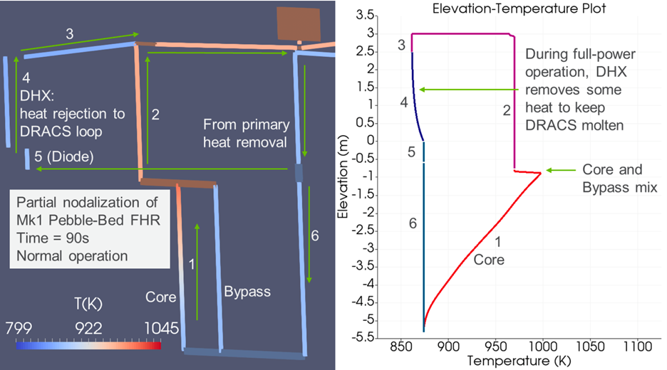
Figure 4: Coolant temperature during steady state (t = 90s).
In this simulation, a protected loss of forced flow occurs at t = 100 s. The power drops immediately to about 5% of nominal power and decay heat is the sole heat source in the core. Figure 5 shows the temperature profile and flow pattern at t=1400 s. Natural circulation is established in the primary-to-DHX loop as indicated by the area enclosed in the elevation-temperature plot. The flow driven upward by the core through pipe 2 then enters path 3-4-5, so that DHX behaves as a countercurrent heat exchanger.
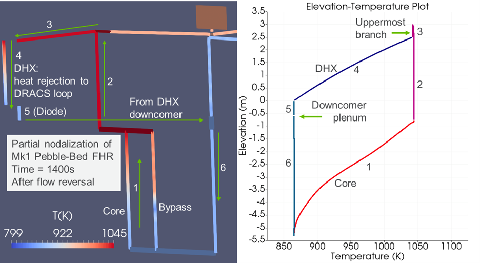
Figure 5: Coolant temperature during loss of forced flow transient (at t = 1400s).
Running the Input File
SAM can be run in Linux, Unix, and MacOS. Due to its dependence on MOOSE, SAM is not compatible with Windows machine. SAM can be run from the shell prompt as shown below
sam-opt -I pbfhr-ss.i
References
- K K Ahmed, R O Scarlat, and R Hu.
Benchmark Simulation of Natural Circulation Cooling System with Salt Working Fluid Using SAM.
In 17th International Topical Meeting on Nuclear Reactor Thermal Hydraulics (NURETH-17). Xi'an, China, 2017. American Nuclear Society.
URL: https://www.osti.gov/biblio/1392061.[BibTeX]
@inproceedings{Ahmed2017, author = "Ahmed, K K and Scarlat, R O and Hu, R", address = "Xi'an, China", booktitle = "17th International Topical Meeting on Nuclear Reactor Thermal Hydraulics (NURETH-17)", language = "English", publisher = "American Nuclear Society", title = "{Benchmark Simulation of Natural Circulation Cooling System with Salt Working Fluid Using SAM}", url = "https://www.osti.gov/biblio/1392061", year = "2017" } - Charalampos “Harry” Andreades, Anselmo T. Cisneros, Jae Keun Choi, Alexandre Y.K. Chong, Massimiliano Fratoni, Sea Hong, Lakshana R. Huddar, Kathryn D. Huff, David L. Krumwiede, Michael R. Laufer, Madicken Munk, Raluca O. Scarlat, Nicolas Zweibaum, Ehud Greenspan, and Per F. Peterson.
Technical Description of the “Mark 1” Pebble-Bed Flouride-Salt-Cooled High Temperature Reactor (PB-FHR) Power plant.
Technical Report, University of California, Berkeley, Berkeley, CA, 2014.[BibTeX]
@techreport{Andreades2014, author = "Andreades, Charalampos “Harry” and Cisneros, Anselmo T. and Choi, Jae Keun and Chong, Alexandre Y.K. and Fratoni, Massimiliano and Hong, Sea and Huddar, Lakshana R. and Huff, Kathryn D. and Krumwiede, David L. and Laufer, Michael R. and Munk, Madicken and Scarlat, Raluca O. and Zweibaum, Nicolas and Greenspan, Ehud and Peterson, Per F.", address = "Berkeley, CA", institution = "University of California, Berkeley", title = "{Technical Description of the “Mark 1” Pebble-Bed Flouride-Salt-Cooled High Temperature Reactor (PB-FHR) Power plant}", year = "2014" } - Rui Hu.
SAM Theory Manual.
Technical Report ANL/NE-17/4, Argonne National Laboratory, Lemont, IL, 2017.[BibTeX]
@techreport{Hu2017, author = "Hu, Rui", address = "Lemont, IL", number = "ANL/NE-17/4", mendeley-tags = "ANL/NE-17/4", institution = "Argonne National Laboratory", title = "{SAM Theory Manual}", year = "2017" } - Nicolas Zweibaum.
Experimental Validation of Passive Safety System Models: Application to Design and Optimization of Fluoride-Salt-Cooled, High-Temperature Reactors.
PhD thesis, UC Berkeley, 2015.[BibTeX]
@phdthesis{Zweibaum2015,
    author = "Zweibaum, Nicolas",
    publisher = "UC Berkeley",
    school = "UC Berkeley",
    title = "{Experimental Validation of Passive Safety System Models: Application to Design and Optimization of Fluoride-Salt-Cooled, High-Temperature Reactors}",
    year = "2015"
}
(pbfhr/mark1/sam_model/pbfhr-ss.i)
# Modeling the UC Berkerkey Mk-1 pebble bed FHR conceptual design
# Includes DRACS loop for emergency heat removal
# Steady state and transient simulation (loss of forced flow with SCRAM)
# Work supported under the DOE NEAMS program
# Application : SAM
# If using or referring to this model, please cite as explained on
# https://mooseframework.inl.gov/virtual_test_bed/citing.html

[GlobalParams] # global parameters initialization
  global_init_P = 1.0e5
  global_init_V = 1.796
  global_init_T = 874
  Tsolid_sf = 1e-3

  scaling_factor_var = '1 1e-2 1e-6' # fluid model solver parameters
  p_order = 2
[]

[EOS]
  [eos]
    type = SaltEquationOfState # use built-in equation of state of Flibe
    salt_type = Flibe
  []
[]

[MaterialProperties]
  [ss-mat]
    type = SolidMaterialProps
    k = 40
    Cp = 583.333
    rho = 6e3
  []
  [h451]
    type = SolidMaterialProps
    k = 173.49544
    Cp = 1323.92
    rho = 4914.2582
  []
  [fuel]
    type = SolidMaterialProps
    k = 32.5304 #15
    Cp = 1323.92
    rho = 4914.2582
  []
[]

[Functions]

  [Paxial] # used to describe axial power shape
    type = PiecewiseConstant # function type
    axis = x # x-co-ordinate is used for x
    direction = right
    xy_data = '0.176153846153846 0.0939862040
  0.352307692307692 0.2648701900
  0.528461538461539 0.4186657800
  0.704615384615385 0.5895497920
  0.880769230769231 0.7689779760
  1.056923076923080 0.9056851700
  1.233076923076920 0.9825829780
  1.409230769230770 1.0082155720
  1.585384615384620 1.0167597700
  1.761538461538460 1.0167597700
  1.937692307692310 1.0509365880
  2.113846153846150 1.1363785680
  2.290000000000000 1.2047321780
  2.466153846153850 1.2218205740
  2.642307692307690 1.2303647720
  2.818461538461540 1.2559973660
  2.994615384615380 1.2389089700
  3.170769230769230 1.1961879800
  3.346923076923080 1.1278343700
  3.523076923076920 1.0509365880
  3.699230769230770 1.0851133800
  3.875384615384620 1.1192901720
  4.051538461538460 1.1876437820
  4.227692307692310 1.2645415640
  4.403846153846150 1.3499835700
  4.580000000000000 1.2132763760'
  []

  [Phead]
    type = PiecewiseLinear
    x = '0   400    404.5  409    413.5 418   422.5 427  431.5 436   440.5 445   448   450.5 452    454   457.5 460   480   500   600   10000'
    y = '367475 367475 182810 89969  43302 19845 8054  2128 -851  -1500 -1700 -1720 -1720 -1730 -1760 -1790 -1830 -1870 -2150 -2350 -2500 -2500'
  []

  [shutdownPower]
    type = PiecewiseLinear
    x = '0    100    101    102    104    108    116    124    132    140    148    160    220    340    580    1060    1540    2020    2500    2980    3460    3700    12300'
    y = '1.0000    1.0000    0.0530    0.0508    0.0479    0.0441    0.0403    0.0378    0.0361    0.0347    0.0336    0.0322    0.0279    0.0242    0.0210    0.0179    0.0161    0.0148    0.0138    0.0130    0.0124    0.0121    0.0081'
  []

[]

[Components]

  [reactor]
    type = ReactorPower
    initial_power = 2.36e8 # Initial total reactor power
  []

  [pipe010] #Active core region (1)
    type = PBCoreChannel
    eos = eos
    position = '0 4.94445 -5.34'
    orientation = '0 0 1'
    roughness = 0.000015
    A = 1.327511
    Dh = 0.03
    length = 4.58
    n_elems = 13 #26
    initial_V = 0.290
    initial_T = 920
    initial_P = 2.6e5

    WF_user_option = User
    User_defined_WF_parameters = '5.467 847.17 -1.0'

    HT_surface_area_density = 133.33 #Preserves surface area
    Ts_init = 950
    elem_number_of_hs = '5 5 2'
    material_hs = 'h451 fuel h451'
    n_heatstruct = 3
    fuel_type = cylinder
    name_of_hs = 'inner fuel outer'
    width_of_hs = '0.007896334 0.001463164 0.001020503'

    power_fraction = '0 1 0'
    power_shape_function = Paxial
    HTC_geometry_type = Bundle
    PoD = 1.1
    dim_hs = 2
  []

  [pipe020] #Core bypass (2)
    type = PBOneDFluidComponent
    eos = eos
    position = '0 5.92445 -5.34'
    orientation = '0 0 1'
    roughness = 0.000015
    A = 0.065
    Dh = 0.01
    length = 4.58
    n_elems = 13 #26
    initial_V = 1.993
    initial_P = 2.6e5
  []

  [Branch030] #Outlet plenum (3)
    type = PBVolumeBranch
    inputs = 'pipe010(out) pipe020(out)' # A = 1.327511 (0.2524495) A = 0.065
    outputs = 'pipe040(in)' # A = 0.2512732
    center = '0 4.94445 -0.76'
    volume = 0.99970002
    K = '0.3668 0.35336 0.0006' # loss coefficients
    Area = 0.2524495 # L = 3.96
    eos = eos
    initial_V = 2.040
    initial_T = 970
    initial_P = 1.7e5
    width = 2
    height = 0.2
    nodal_Tbc = true
  []

  [pipe040] #Hot salt extraction pipe (4)
    type = PBOneDFluidComponent
    eos = eos
    position = '0 3.96445 -0.76'
    orientation = '0 0 1'
    roughness = 0.000015
    A = 0.2512732
    Dh = 0.5656244
    length = 3.77
    n_elems = 11 #21
    initial_V = 2.050
    initial_T = 970
    initial_P = 1.3e5
  []

  [pipe050] #Reactor vessel to hot salt well (5)
    type = PBOneDFluidComponent
    eos = eos
    position = '0 4.46445 3.01'
    orientation = '0 3.72912 0.081'
    roughness = 0.000015
    A = 0.264208
    Dh = 0.58
    length = 3.73
    n_elems = 11 #21
    initial_V = 2.05
    initial_T = 970
  []

  [pipe060] #Hot well (6)
    type = PBOneDFluidComponent
    eos = eos
    position = '0 8.30 3.09' #'0 8.19357 3.091'
    orientation = '0 1.970888 0.34'
    roughness = 0.000015
    A = 3.3145
    Dh = 1.452610
    length = 2.00
    n_elems = 6 #11
    initial_V = 0.164
    initial_T = 970
  []

  [pipe070] #Hot salt well to CTAH (7)
    type = PBOneDFluidComponent
    eos = eos
    position = '0 10.271 3.43'
    orientation = '0 3.22967 -0.046'
    roughness = 0.000015
    A = 0.3041
    Dh = 0.4399955
    length = 3.23
    n_elems = 9 #18
    initial_V = 1.783
    initial_T = 970
    initial_P = 4.6e5
  []

  [pipe080] #CTAH hot manifold (8)
    type = PBOneDFluidComponent
    eos = eos
    position = '0 13.5 3.384'
    orientation = '0 0 -1'
    roughness = 0.000015
    A = 0.4926017
    Dh = 0.28
    length = 3.418
    n_elems = 10 #19
    initial_V = 1.100
    initial_T = 970
    initial_P = 4.9e5
  []

  [pipe090] #CTAH tubes (salt side) (9)
    type = PBPipe
    eos = eos
    position = '0 13.5 -0.034'
    orientation = '0 18.4692719 -0.164'
    roughness = 0.000015
    A = 0.4491779
    Dh = 0.004572
    length = 18.47
    n_elems = 50 #99
    initial_V = 1.207
    initial_T = 920
    initial_P = 4.1e5

    HS_BC_type = Temperature
    Hw = 2000 #cut for transient
    Ph = 392.9818537
    T_wall = 873.15
    Twall_init = 900
    hs_type = cylinder
    material_wall = ss-mat
    dim_wall = 2
    n_wall_elems = 4
    radius_i = 0.002286
    wall_thickness = 0.000889
  []

  [pipe100] #CTAH cold manifold (10)
    type = PBOneDFluidComponent
    eos = eos
    position = '0 18.2055 -0.197'
    orientation = '0 0 -1'
    roughness = 0.000015
    A = 0.1924226
    Dh = 0.175
    length = 3.418
    n_elems = 10 #19
    initial_V = 2.818
    initial_P = 2.8e5
  []

  [pipe110] #CTAH to drain tank (11)
    type = PBOneDFluidComponent
    eos = eos
    position = '0 18.2055 -3.615'
    orientation = '0 -3.4791917 -0.075'
    roughness = 0.000015
    A = 0.3019068
    Dh = 0.438406
    length = 3.48
    n_elems = 10 #20
    initial_P = 3.1e5
  []

  [pipe120] #Stand pipe (12)
    type = PBOneDFluidComponent
    eos = eos
    position = '0 14.7263 -3.69'
    orientation = '0 0 1'
    roughness = 0.000015
    A = 0.3019068
    Dh = 0.438406
    length = 6.51
    n_elems = 19 #37
    initial_P = 2.5e5
  []

  [pipe130] #Stand pipe to reactor vessel (13)
    type = PBOneDFluidComponent
    eos = eos
    position = '0 14.7263 2.82'
    orientation = '0 -6.6018536 0.14'
    roughness = 0.000015
    A = 0.3019068
    Dh = 0.438406
    length = 6.6033378
    n_elems = 19 #37
    initial_P = 1.8e5
  []

  [pipe140] #Injection plenum (14)
    type = PBOneDFluidComponent
    eos = eos
    position = '0 8.12445 2.96'
    orientation = '0 0 -1'
    roughness = 0.000015
    A = 0.3019068
    Dh = 0.438406
    length = 3.04
    n_elems = 9 #17
    initial_P = 2.1e5
  []

  [pipe150] #Downcomer (15)
    type = PBOneDFluidComponent
    eos = eos
    position = '0 8.12445 -0.58'
    orientation = '0 0 -1'
    roughness = 0.000015
    A = 0.3038791
    Dh = 0.0560284
    length = 4.76
    n_elems = 14 #27
    initial_V = 1.695
    initial_P = 2.9e5
  []

  [pipe160] #Downcomer to DHX (16)
    type = PBOneDFluidComponent
    eos = eos
    position = '0 1 -0.58'
    orientation = '0 0 1'
    roughness = 0.000015
    A = 0.03534292
    Dh = 0.15
    length = 0.58
    n_elems = 3 #3
    initial_V = 0.767
    initial_P = 2.5e5
  []

  [DHX] # DHX shell side (17), DHX tube side (19), DHX tubes structure
    type = PBHeatExchanger
    eos = eos
    eos_secondary = eos
    hs_type = cylinder

    radius_i = 0.00545
    position = '0 0.5 0'
    orientation = '0 0 1'
    A = 0.2224163
    Dh = 0.01085449
    A_secondary = 0.1836403
    Dh_secondary = 0.0109
    roughness = 0.000015
    roughness_secondary = 0.000015
    length = 2.5
    n_elems = 7 #14

    initial_V = 0.122 #0.11969487
    initial_V_secondary = 0.029349731
    initial_T = 870
    initial_T_secondary = 830
    initial_P = 1.9e5
    initial_P_secondary = 2.0e5

    HT_surface_area_density = 441.287971
    HT_surface_area_density_secondary = 458.715596
    #Hw = 526.266
    #Hw_secondary = 440
    HTC_geometry_type = Pipe
    HTC_geometry_type_secondary = Pipe
    PoD = 1.1

    Twall_init = 900
    wall_thickness = 0.0009
    dim_wall = 2
    material_wall = ss-mat
    n_wall_elems = 4
  []

  [pipe180] #DHX to hot leg (18)
    type = PBOneDFluidComponent
    eos = eos
    position = '0 1 2.5'
    orientation = '0 2.96445 .51'
    roughness = 0.000015
    A = 0.03534292
    Dh = 0.15
    length = 3.008
    n_elems = 9 #17
    initial_V = 0.767
    initial_T = 860
    initial_P = 2.6e5
  []

  [pipe200] #DRACS hot leg 1 (20)
    type = PBOneDFluidComponent
    eos = eos
    position = '0 0 2.5'
    orientation = '0 0 1'
    roughness = 0.000015
    A = 0.03534292
    Dh = 0.15
    length = 3.45
    n_elems = 10 #20
  []

  [pipe210] #DRACS hot leg 2 (21)
    type = PBOneDFluidComponent
    eos = eos
    position = '0 -0.2 5.95'
    orientation = '0 -1 0'
    roughness = 0.000015
    A = 0.03534292
    Dh = 0.15
    length = 3.67
    n_elems = 11 #21
  []

  [pipe220] #TCHX Manifold (22)
    type = PBOneDFluidComponent
    eos = eos
    position = '0 -3.87 5.95'
    orientation = '0 0 1'
    roughness = 0.000015
    A = 0.03534292
    Dh = 0.15
    length = 2.60
    n_elems = 8 #15
  []

  [pipe230] #TCHX salt tube (23)
    type = PBPipe
    eos = eos
    position = '0 -3.87 8.55'
    orientation = '0 -5.407402334 -2.6'
    roughness = 0.000015
    A = 0.1746822
    Dh = 0.0109
    length = 6.0
    n_elems = 17 #34
    initial_V = 0.04855862

    HS_BC_type = Temperature
    Hw = 1000
    #Ph = 64.10356978
    HT_surface_area_density = 366.972535
    T_wall = 799.15
    Twall_init = 800
    hs_type = cylinder
    material_wall = ss-mat
    dim_wall = 2
    n_wall_elems = 4
    radius_i = 0.00545
    wall_thickness = 0.0009
  []

  [pipe240] #DRACS cold leg 1 (24)
    type = PBOneDFluidComponent
    eos = eos
    position = '1 -4.43 5.95'
    orientation = '0 1 0'
    roughness = 0.000015
    A = 0.03534292
    Dh = 0.15
    length = 4.43
    n_elems = 13 #25
  []

  [pipe250] #DRACS cold leg 2 (25)
    type = PBOneDFluidComponent
    eos = eos
    position = '1 0 5.95'
    orientation = '0 0 -1'
    roughness = 0.000015
    A = 0.03534292
    Dh = 0.15
    length = 5.95
    n_elems = 17 #34
  []

  [Branch260] #Top branch (26)
    type = PBVolumeBranch
    inputs = 'pipe180(out) pipe040(out)' # A = 0.03534292 A = 0.2512732
    outputs = 'pipe050(in)' # A = 0.264208
    center = '0 4.21445 3.01'
    volume = 0.132104
    K = '0.3713 0.00636 0.0' # loss coefficients
    Area = 0.264208 # L = 0.5
    eos = eos
    initial_V = 2.052
    initial_T = 970
    height = 0.1
    nodal_Tbc = true
  []

  [Branch270] #Middle branch (27)
    type = PBVolumeBranch
    inputs = 'pipe140(out)' # A = 0.3019068
    outputs = 'pipe150(in) pipe160(in)' # A = 0.3038791 A = 0.03534292
    center = '0 8.12445 -0.33'
    volume = 0.15193955
    K = '0.0 0.0 0.3727'
    Area = 0.3038791 # L = 0.5
    eos = eos
    initial_V = 1.784
    initial_P = 2.5e5
    width = 0.2
  []

  [Branch280] #Bottom branch (28)
    type = PBVolumeBranch
    inputs = 'pipe150(out)' # A = 0.3038791
    outputs = 'pipe010(in) pipe020(in)' # A = 1.327511  A = 0.065
    center = '0 6.53445 -5.34'
    volume = 0.2655022
    #K = '0.35964 0.0 0.3750'
    K = '0.35964 0.0 0.6000'
    Area = 1.327511 # L = 0.2
    eos = eos
    initial_V = 0.388
    initial_P = 3.4e5
    width = 3.18
    height = 0.2
  []

  [pipe2] #Pipe to primary tank
    type = PBOneDFluidComponent
    eos = eos #eos3
    position = '0 8.25 3.19'
    orientation = '0 0 1'
    A = 1
    Dh = 1.12838
    length = 0.1
    n_elems = 1
    initial_V = 0.0
    initial_T = 970
  []

  [pool2] #Primary Loop Expansion Tank
    type = PBLiquidVolume
    center = '0 8.25 3.74'
    inputs = 'pipe2(out)'
    Steady = 1
    K = '0.0'
    Area = 1
    volume = 0.9
    initial_level = 0.4
    initial_T = 970
    initial_V = 0.0
    covergas_component = 'cover_gas2'
    eos = eos
  []

  [cover_gas2]
    type = CoverGas
    name_of_liquidvolume = 'pool2'
    initial_P = 9e4
    initial_Vol = 0.5
    initial_T = 970
  []

  [Branch501] #Primary tank branch
    type = PBVolumeBranch
    inputs = 'pipe050(out)' # A = 0.264208
    outputs = 'pipe060(in) pipe2(in)' # A = 3.3145 (0.264208) A = 1 (0.264208)
    center = '0 8.25 3.09'
    volume = 0.0264208
    K = '0 0.3744 0.35187'
    Area = 0.264208 # L = 0.2
    eos = eos
    initial_V = 2.052
    initial_T = 970
    width = 0.1
  []

  [pipe1] #Pipe to DRACS tank
    type = PBOneDFluidComponent
    eos = eos #eos3
    position = '0 0 5.95'
    orientation = '0 0 1'
    A = 1
    Dh = 1.12838
    length = 0.1
    n_elems = 1
    initial_T = 852.7
  []

  [pool1] #DRACS tank
    type = PBLiquidVolume
    center = '0 0 6.5'
    inputs = 'pipe1(out)'
    Steady = 1
    K = '0.0'
    Area = 1
    volume = 0.9
    initial_level = 0.4
    initial_T = 852.7
    initial_V = 0.0
    covergas_component = 'cover_gas1'
    eos = eos #eos3
  []

  [cover_gas1]
    type = CoverGas
    name_of_liquidvolume = 'pool1'
    initial_P = 2e5
    initial_Vol = 0.5
    initial_T = 852.7
  []

  [Branch502] #DRACS tank branch
    type = PBVolumeBranch
    inputs = 'pipe200(out)' # A = 0.1836403
    outputs = 'pipe210(in) pipe1(in)' # A = 0.1836403 A = 1
    center = '0 -0.1 5.95'
    volume = 0.003534292
    K = '0.0 0.0 0.3673'
    Area = 0.03534292
    eos = eos
  []

  [Branch601] # In to hot manifold
    type = PBBranch
    inputs = 'pipe070(out)' # A = 0.3041
    outputs = 'pipe080(in)' # A = 0.4926017
    eos = eos
    K = '0.16804 0.16804'
    Area = 0.3041
    initial_V = 1.783
    initial_T = 970
    initial_P = 4.6e5
  []

  [Branch602] # In to CTAH salt side
    type = PBBranch
    inputs = 'pipe080(out)' # A = 0.4926017
    outputs = 'pipe090(in)' # A = 0.4491779
    eos = eos
    K = '0.01146 0.01146'
    Area = 0.4491779
    initial_V = 1.207
    initial_T = 970
    initial_P = 5.2e5
  []

  [Branch603] # In to cold manifold
    type = PBBranch
    inputs = 'pipe090(out)' # A = 0.4491779
    outputs = 'pipe100(in)' # A = 0.1924226
    eos = eos
    K = '0.28882 0.28882'
    Area = 0.1924226
    initial_V = 2.818
    initial_P = 2.5e5
  []

  [Branch604] # In to pipe to drain tank
    type = PBBranch
    inputs = 'pipe100(out)' # A = 0.1924226
    outputs = 'pipe110(in)' # A = 0.3019068
    eos = eos
    K = '0.15422 0.15422'
    K_reverse = '2000000 2000000'
    Area = 0.1924226
    initial_P = 3.1e5
  []

  [Branch605] # In to stand pipe
    type = PBSingleJunction
    inputs = 'pipe110(out)'
    outputs = 'pipe120(in)'
    eos = eos
    initial_P = 3.1e5
  []

  [Branch606] # In to pipe to reactor vessel
    type = PBSingleJunction
    inputs = 'pipe120(out)'
    outputs = 'pipe130(in)'
    eos = eos
    initial_P = 1.9e5
  []

  [Branch607] # In to injection plenum
    type = PBSingleJunction
    inputs = 'pipe130(out)'
    outputs = 'pipe140(in)'
    eos = eos
    initial_P = 1.8e5
  []

  [Diode608] # Fluidic diode
    type = PBBranch
    inputs = 'pipe160(out)' # A = 0.03534292
    outputs = 'DHX(primary_in)' # A = 0.2224163
    eos = eos
    K = '50.0 50.0'
    K_reverse = '1.0 1.0'
    Area = 0.03534292
    initial_V = 0.767
    initial_P = 2.3e5
  []

  [Branch609] # Out of DHX
    type = PBBranch
    inputs = 'DHX(primary_out)' # A = 0.2224163
    outputs = 'pipe180(in)' # A = 0.03534292
    eos = eos
    K = '94.8693 94.8693'
    Area = 0.03534292
    initial_V = 0.767
    initial_P = 1.3e5
  []

  [Branch610] #In to DRACS hot leg 1
    type = PBBranch
    inputs = 'DHX(secondary_in)' # A = 0.1836403
    outputs = 'pipe200(in)' # A = 0.03534292
    eos = eos
    K = '56.3666 56.3666'
    Area = 0.03534292
  []

  [Branch611] #In to TCHX manifold
    type = PBSingleJunction
    inputs = 'pipe210(out)'
    outputs = 'pipe220(in)'
    eos = eos
  []

  [Branch612] #In to TCHX salt tube
    type = PBBranch
    inputs = 'pipe220(out)' # A = 0.03534292
    outputs = 'pipe230(in)' # A = 0.1746822
    eos = eos
    K = '0.3655 0.3655'
    #K = '0.0 0.3655'
    Area = 0.03534292
  []

  [Branch613] #In to DRACS cold leg 1
    type = PBBranch
    inputs = 'pipe230(out)' # A = 0.1746822
    outputs = 'pipe240(in)' # A = 0.03534292
    eos = eos
    K = '0.3655 0.3655'
    #K = '0.3655 0.0'
    Area = 0.03534292
  []

  [Branch614] #In to DRACS cold leg 2
    type = PBSingleJunction
    inputs = 'pipe240(out)'
    outputs = 'pipe250(in)'
    eos = eos
  []

  [Branch615] #In to DHX tube side
    type = PBBranch
    inputs = 'pipe250(out)' # A = 0.03534292
    outputs = 'DHX(secondary_out)' # A = 0.1836403
    eos = eos
    K = '0.3666 0.3666'
    #K = '0.0 0.3666'
    Area = 0.03534292
  []

  [Pump]
    type = PBPump
    inputs = 'pipe060(out)'
    outputs = 'pipe070(in)'
    eos = eos
    K = '0 0'
    K_reverse = '2000000 2000000'
    Area = 0.3041
    Head = Phead
    initial_V = 1.783
    initial_T = 970
    initial_P = 2.7e5
  []

[]

[Postprocessors]
  [DHX_flow]
    type = ComponentBoundaryFlow
    input = DHX(primary_out)
    execute_on = timestep_end
  []
  [DHX_q]
    type = HeatExchangerHeatRemovalRate
    heated_perimeter = 78.51971015
    block = 'DHX:primary_pipe'
    execute_on = timestep_end
  []
  [DHXshellBot]
    type = ComponentBoundaryVariableValue
    input = 'DHX:primary_pipe(in)'
    variable = 'temperature'
  []
  [DHXshellTop]
    type = ComponentBoundaryVariableValue
    input = 'DHX:primary_pipe(out)'
    variable = 'temperature'
  []
  [DHXTubeBot]
    type = ComponentBoundaryVariableValue
    input = 'DHX:secondary_pipe(in)'
    variable = 'temperature'
  []
  [DHXTubeTop]
    type = ComponentBoundaryVariableValue
    input = 'DHX:secondary_pipe(out)'
    variable = 'temperature'
  []
  [Corev]
    type = ComponentBoundaryVariableValue
    input = 'pipe010(in)'
    variable = 'velocity'
  []
  [Corerho]
    type = ComponentBoundaryVariableValue
    input = 'pipe010(in)'
    variable = 'rho'
  []
  [Bypassv]
    type = ComponentBoundaryVariableValue
    input = 'pipe020(in)'
    variable = 'velocity'
  []
  [Bypassrho]
    type = ComponentBoundaryVariableValue
    input = 'pipe020(in)'
    variable = 'rho'
  []
[]

[Preconditioning]
  active = 'SMP_PJFNK'
  [SMP_PJFNK]
    type = SMP
    full = true
    solve_type = 'PJFNK'
    petsc_options_iname = '-pc_type'
    petsc_options_value = 'lu'
  []
  [FDP]
    type = FDP
    full = true
    solve_type = 'PJFNK'
  []

[]

[Executioner]
  type = Transient

  petsc_options_iname = '-ksp_gmres_restart -pc_factor_shift_type -pc_factor_shift_amount'
  petsc_options_value = '300 NONZERO 1e-9'

  dt = 1
  dtmin = 1e-3

  [TimeStepper]
    type = FunctionDT
    function = 'dts'
  []

  # Time integration scheme
  scheme = 'bdf2'

  nl_rel_tol = 1e-5
  nl_abs_tol = 1e-4
  nl_max_its = 30

  start_time = -300.0
  num_steps = 15000
  end_time = 100

  l_tol = 1e-5 # Relative linear tolerance for each Krylov solve
  l_max_its = 200 # Number of linear iterations for each Krylov solve

  [Quadrature]
    type = GAUSS # SIMPSON
    order = SECOND
  []
[]

[Functions]
  [dts]
    type = PiecewiseConstant
    x = '   0   400 401 998  999   1250  1251  1500 1501 4000 4001 1e5'
    y = '   1   1   5   5    0.2   0.2   0.5   0.5  1    1     5    5'
    direction = 'LEFT_INCLUSIVE'
  []
[]

#[Problem]
#restart_file_base = 'pbfhr-t_out_cp/0658'  #c1 right after transient
#[]

[Outputs]
  print_linear_residuals = false
  [out]
    type = Checkpoint
  []

  [out_displaced]
    type = Exodus
    use_displaced = true
    execute_on = 'initial timestep_end'
    time_step_interval = 5
    sequence = false
  []
  [csv]
    type = CSV
    time_step_interval = 5
  []

  [console]
    type = Console
    time_step_interval = 20
  []
[]