Seismic analysis of a base-isolated nuclear power plant building
This model was adopted from the list of examples on the MASTODON website. The inputs can be found here.
GN, GPa, m, and sec
Part 1: Foundation basemat analysis
Before performing the seismic analysis of the full NPP building, the base-isolated basemat is first analyzed.
Modeling
The isolation system of the building comprises 70 Friction PendulumTM (FP) isolators arranged in a grid shown in Figure 2 below. Note that the figure shows a view of the foundation from the bottom, and therefore the +Z axis is pointing inwards into the basemat. The basemat is 98.75m x 68.75m in plan and is 1m thick.
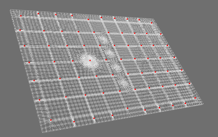
Figure 2: Isolators under the basemat of the NPP building analyzed in Part 1 of this model.
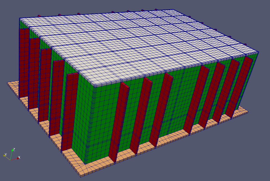
Figure 3: Isometric view of the NPP building mesh analyzed in Part 2 of this model.
The basemat is modeled to be almost rigid, with an elastic modulus of almost 99.2 GPa, which is four times stiffer than concrete. Each of the isolators is independently attached to the basemat with rigid beam elements, thereby simulating a rigid connection between them. The isolators themselves are 0.3m long and have a friction coefficient, mu_ref=0.06, radius of curvature, and r_eff=1.0. These properties result in a sliding period of 2 sec, which is reasonable for the NPP building. Two methods of modeling the isolation system are demonstrated here. In method 1, the friction coefficients of the isolators are assumed to be independent of pressure, temperature, and velocity and the mu_ref value is used throughout the simulations. (See the theory manual for a detailed description of pressure, temperature, velocity dependency of the friction coefficient of FP isolators). Additionally, a unidirectional ground motion is applied in the X direction. In method 2, the pressure, temperature, and velocity dependencies are switched on and ground motions are applied in all three directions. The Materials blocks for the isolators for the two methods are listed below, and the acceleration histories of the input motions are presented in Figure 1 below.
[Materials]
  [elasticity]
    type = ComputeFPIsolatorElasticity
    mu_ref = 0.06
    p_ref = 0.05 # GPa
    block = 'isolator_elems'
    diffusivity = 4.4e-6
    conductivity = 18
    a = 100
    r_eff = 1.0 # meters. 2sec sliding period
    r_contact = 0.2
    uy = 0.001
    unit = 4
    beta = 0.275625
    gamma = 0.55
    pressure_dependent = false
    temperature_dependent = false
    velocity_dependent = false
    k_x = 78.53 # 7.853e10 N
    k_xx = 0.62282 # 622820743.6 N
    k_yy = 0.3114 # 311410371.8 N
    k_zz = 0.3114 # 311410371.8 N
  []
[][Materials]
[elasticity]
type = ComputeFPIsolatorElasticity
mu_ref = 0.06
p_ref = 0.1 # GPa
block = 'isolator_elems'
diffusivity = 4.4e-6
conductivity = 18
a = 100
r_eff = 1.0 # meters. 2sec sliding period
r_contact = 0.2
uy = 0.001
unit = 4
beta = 0.275625
gamma = 0.55
pressure_dependent = true
temperature_dependent = true
velocity_dependent = true
k_x = 78.53 # 7.853e10 N
k_xx = 0.62282 # 622820743.6 N
k_yy = 0.3114 # 311410371.8 N
k_zz = 0.3114 # 311410371.8 N
[]
[]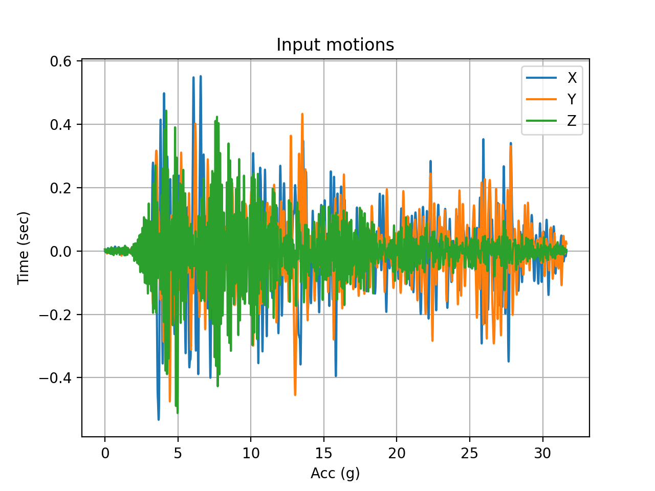
Figure 1: Acceleration histories of the input ground motions used in this model.
Continuum elements such as HEX8 in 3D and QUAD4 in 2D, do not have rotational degrees of freedom. When connecting other elements such as beams or link elements (such as isolators) or shell elements, which do have rotational dofs, to continuum elements, these connection nodes are at a risk of having zero stiffness unless they involve another element with a rotational dof connected to them. In the case of this model, where each of the rigid beam elements (that connect the isolators to the basemat) are directly connected to the solid elements the rotational stiffness of this node (i.e., the Jacobian for the rotational dof of the node) is zero. Having zeros in the Jacobian can lead to significant convergence issues, and with enough zeros, non convergence. In this model, this is avoided by constraining the rotational dofs of these specific nodes as can be seen in the input file. Users are recommended to constrain such rotational dofs when their stiffness is zero to avoid convergence issues.
Gravity analysis is an integral part of seismic analysis of base-isolated structures, especially with FP bearings. The shear strength of the FP bearings depends on the normal force on the surface, which comes from gravity. In this model, gravity loads are initiated through a static initialization performed in the first 3 time steps. Static analysis is achieved by (a) switching off the velocity and acceleration calculations in the time integrator for the first couple of timesteps in the NewmarkBeta TimeIntegrator block, and (b) switching off the inertia kernels using the controls block. Static initialization also requires that the stiffness damping is turned off in the stress divergence kernels, typically by setting static_initialization=true when available. This option is currently only available for continuum elements through the DynamicTensorMechanics block and the isolators through the StressDivergenceIsolator block. Static initialization is turned on for both of these kernels in this model. Note from the input file, that time derivative calculations are turned off for the first two timesteps and the inertia kernels are switched on in the 3rd time step. It is highly recommended that users go through these parts of the input file that enable gravity simulation.
Outputs
An important output in seismic analysis of isolated systems is the force-displacement relationship from the isolators. The forces and deformations in the isolators can be recorded directly using MaterialRealCMMAux, which can retrieve the isolator deformations, forces, stiffnesses (all of which, are of MOOSE ColumnMajorMatrix type in their implementation; see source code) and store them in an AuxVariable. In this model, the isolator deformations and forces in the basic co-ordinate system are recorded and presented. A sample MaterialRealCMMAux definition for the calculation and storage of the axial forces in the isolators is shown below. On examination of the source code for ComputeFPIsolatorElasticity it can be seen that the forces in the basic co-ordinate system are stored in the material property named basic_forces. This is 6 x 1 matrix that stores the forces and moments of the isolators. The first element (row=0 and column=0) corresponds to the axial forces in the isolators and is calculated and stored here. Similarly, the deformations are also evaluated in other blocks.
[AuxKernels]
  [Fb_x]
    type = MaterialRealCMMAux
    property = basic_forces
    row = 0
    column = 0
    variable = Fb_x
    block = 'isolator_elems'
  []
[]Both the acceleration responses of the basemat and the force-displacement relationship of one of the isolators is presented in this section. In Figure 4 and Figure 5, the orange and blue lines correspond to methods 1 and 2, respectively. Note that when the pressure, temperature, and velocity dependencies are switched on (method 2, blue) the hysteresis is a lot more complicated and the stiffness varies significantly during the earthquake. Note that the results for method 1 do not appear in Figure 5 because they are almost zero, given that the ground motion for method 1 is unidirectional. The results presented here are for an isolator at the center of the basemat plan.
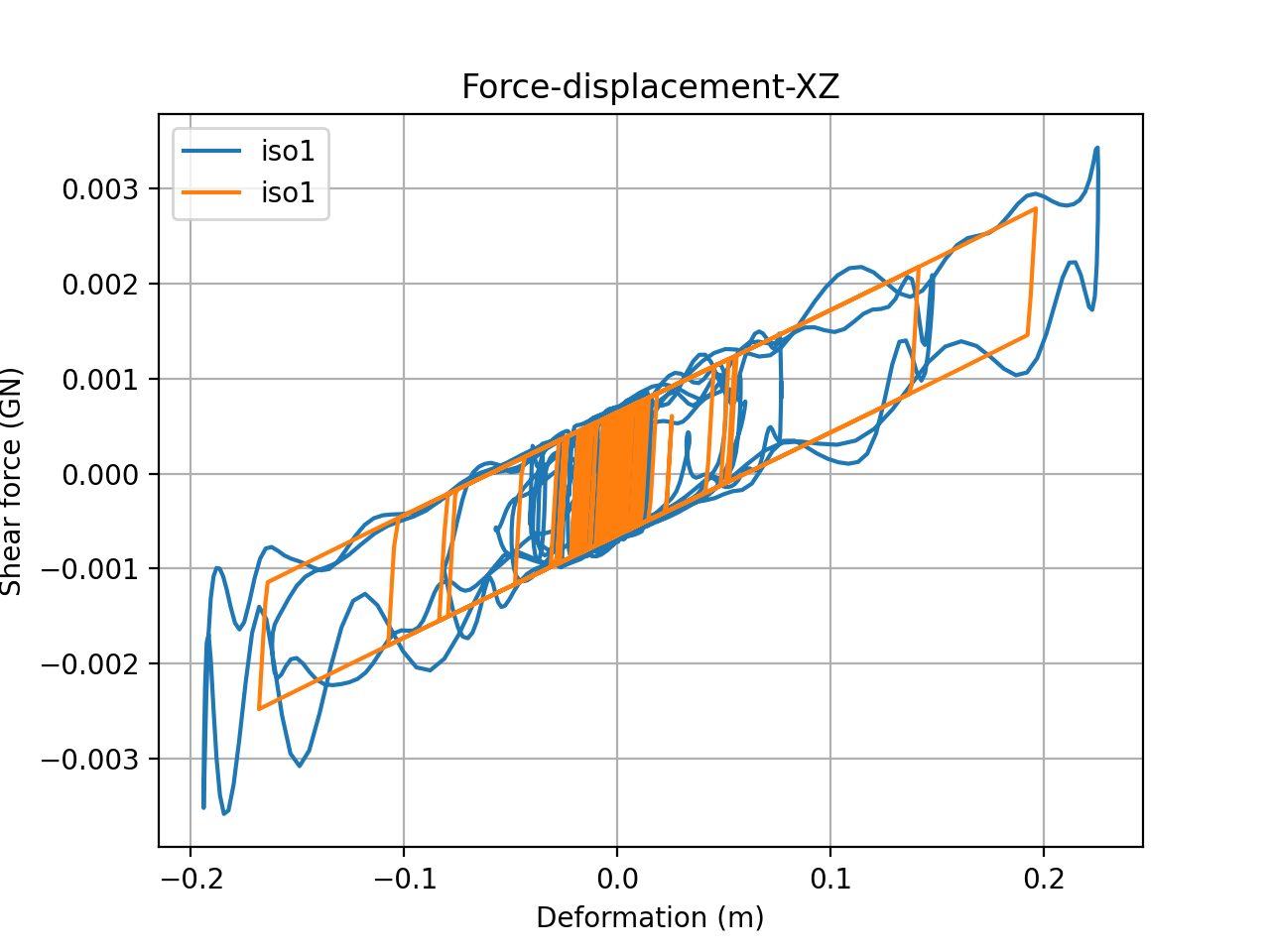
Figure 4: Shear force-displacement history in the XZ direction. Orange is method 1 and blue is method 2.
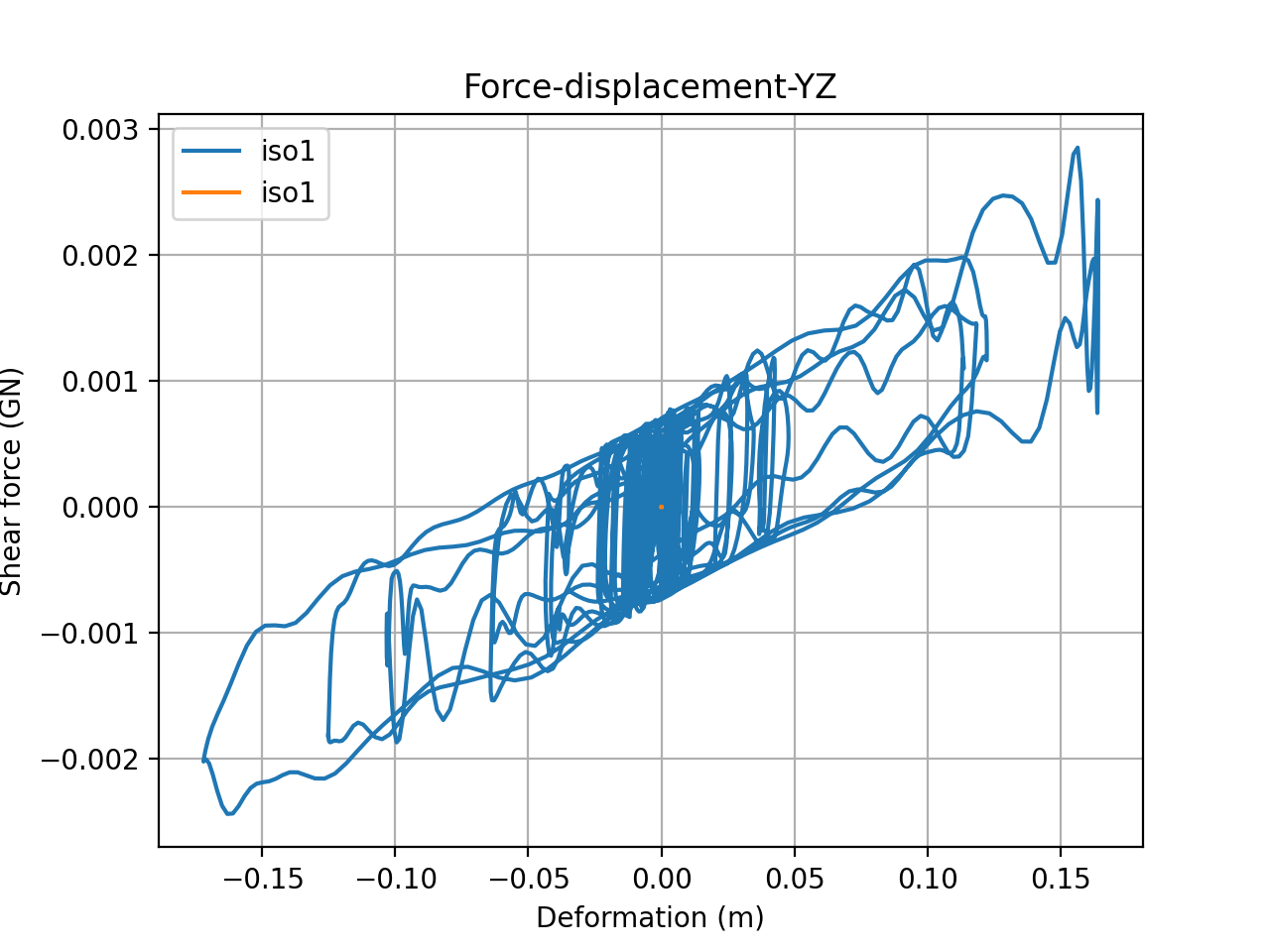
Figure 5: Shear force-displacement history in the YZ direction. Orange is method 1 and blue is method 2.
The acceleration response spectra calculated at the center of the basemat are presented in the figures below. The top row presents the input acceleration spectra and the bottom row presents the output spectra at the center of the basemat in X, Y, and Z directions. Again, in these figures, blue plots present method 1 and orange plots present method 2. The figures show that the accelerations at the top of the basemat reduce drastically due to seismic isolation, except in the Z direction, in which, the response almost stays the same, demonstrating a typical isolation response with FP isolation systems.
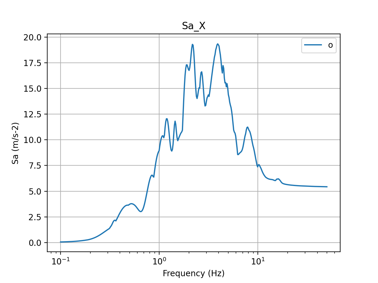
Figure 6: 5% damped acceleration response spectra in X direction (input)
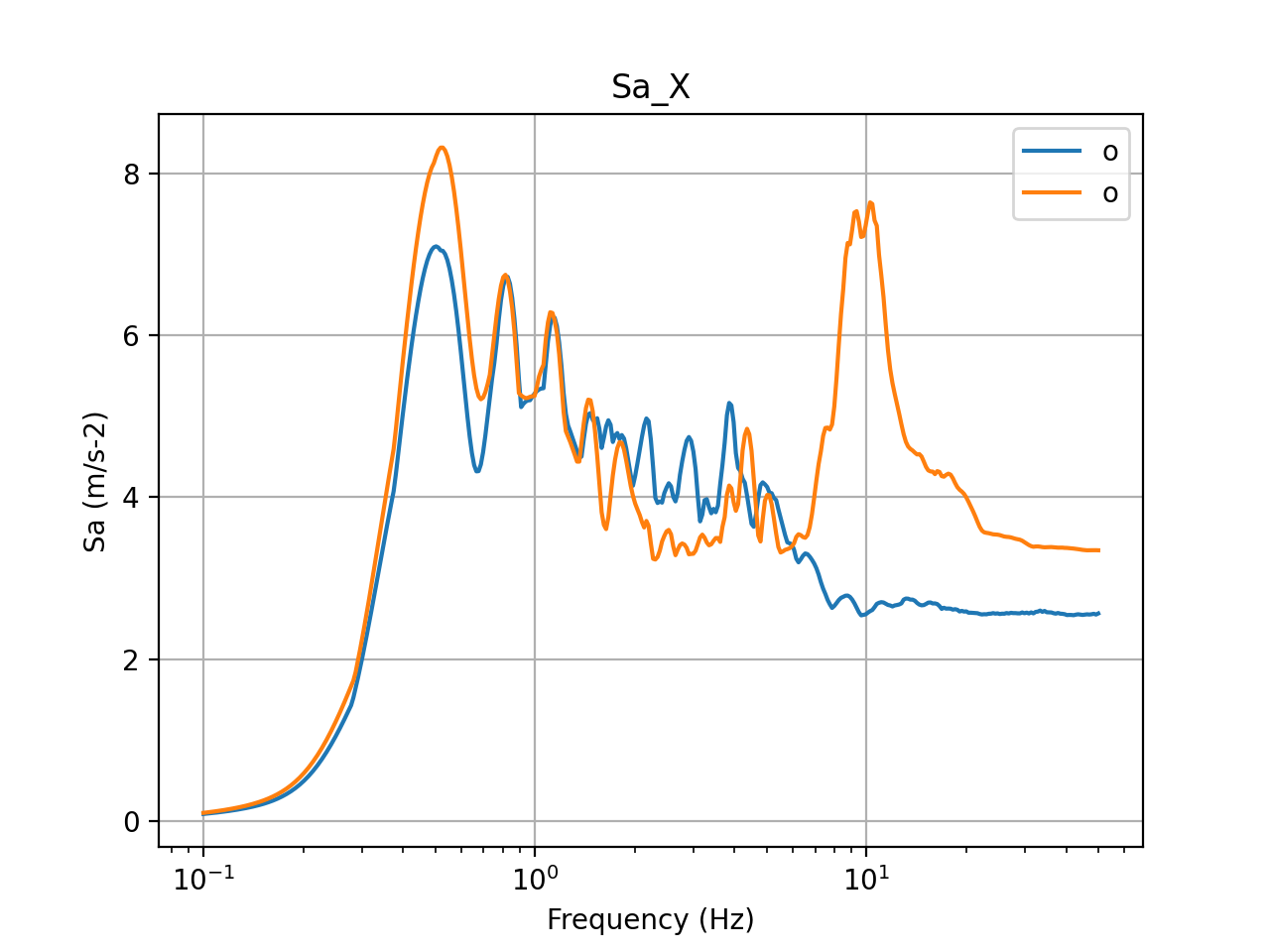
Figure 7: 5% damped acceleration response spectra in X direction (basemat center)
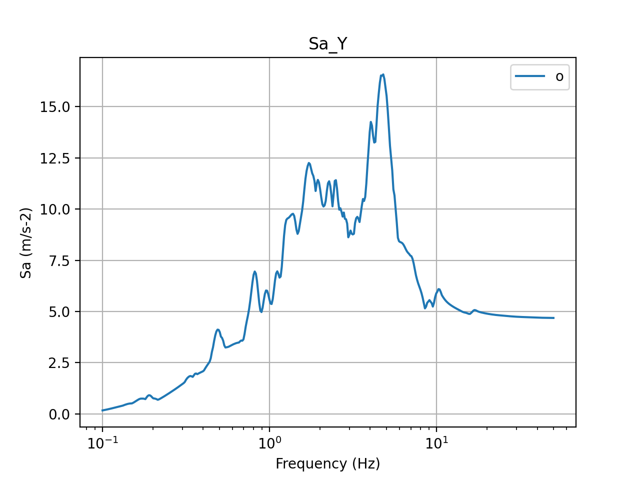
Figure 8: 5% damped acceleration response spectra in Y direction (input)
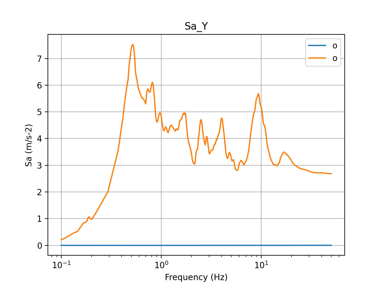
Figure 9: 5% damped acceleration response spectra in Y direction (basemat center)
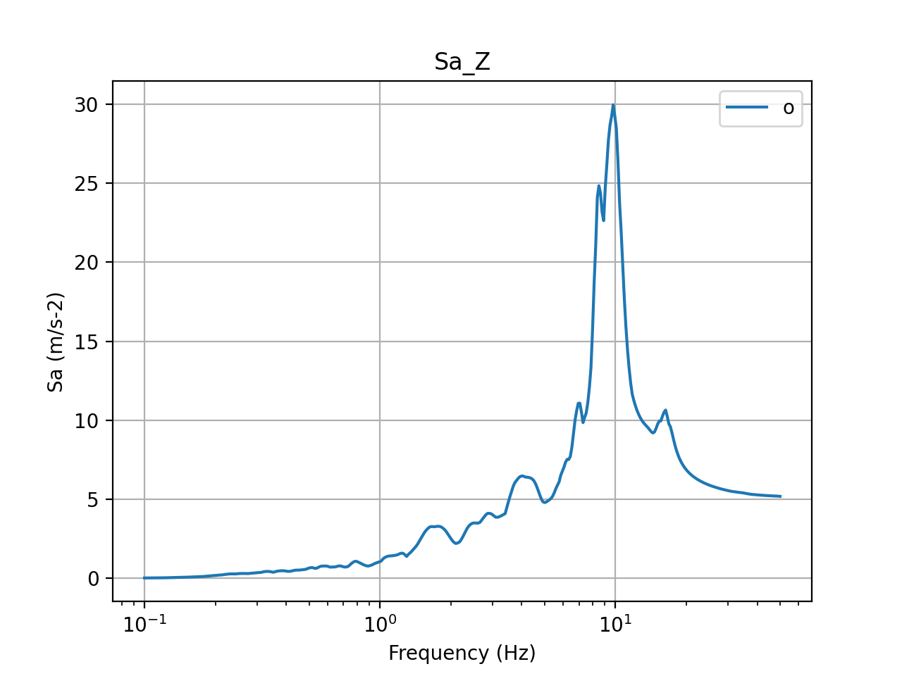
Figure 10: 5% damped acceleration response spectra in Z direction (input)
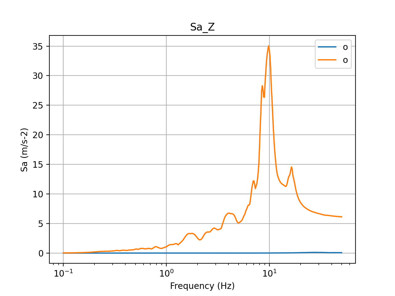
Figure 11: 5% damped acceleration response spectra in Z direction (basemat center)