Heat-Pipe Microreactor Assembly
Contact: Joshua Hansel (joshua.hansel.at.inl.gov)
Model link: Heat-Pipe Microreactor Assembly
Problem Description
This problem consists of a fictitious heat-pipe-cooled micro-reactor (HPMR) assembly, partially taken from (Stauff et al., 2021), with 7 heat pipes and 24 fuel pins. Figure 1 shows the meshed core from the secondary side, with the holes corresponding to the heat pipe locations. Axially, the core is bounded by reflector regions.
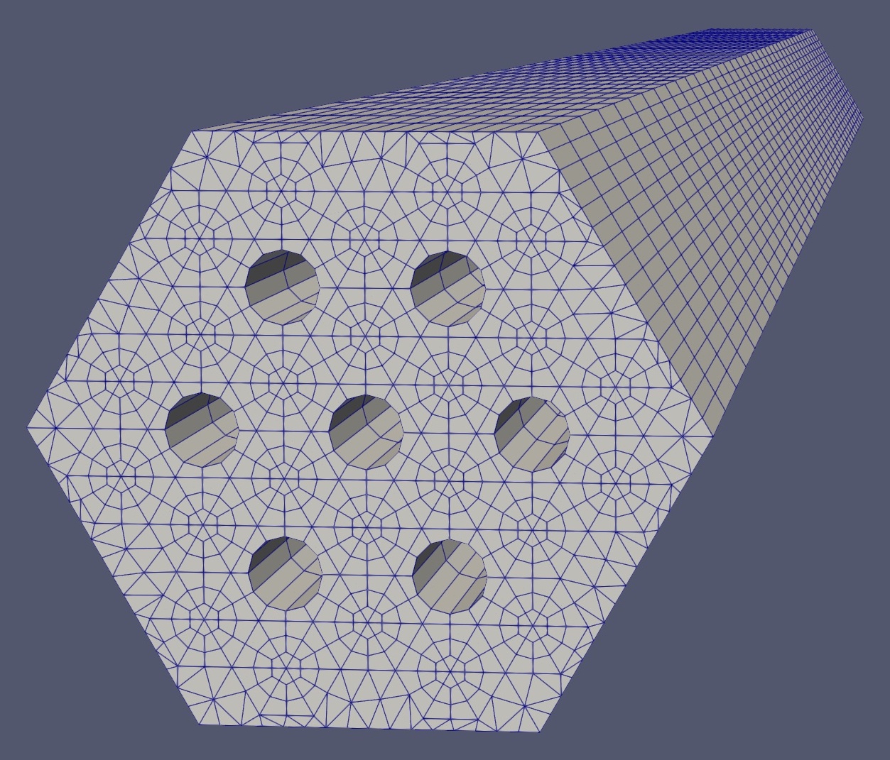
Figure 1: Assembly core mesh.
Table 1 gives the parameters of the core, including geometry and materials, and Table 2 gives the parameters of the heat pipes.
Table 1: Core parameters.
| Parameter | Value |
|---|---|
| Fuel pin length | 160 cm |
| Heat pipe length | 400 cm |
| Heat pipe condenser length | 180 cm |
| Bottom reflector length | 20 cm |
| Top reflector length | 20 cm |
| Fuel pin radius (with gap) | 0.95 cm |
| Heat pipe gap thickness | 0.01 cm |
| Assembly pitch (twice the apothem) | 17.368 cm |
| Unit cell pitch (twice the apothem) | 2.782 cm |
| Core matrix material | IG-110 graphite |
| Fuel material | TRISO particles, in graphite compact |
| Gap fluid | helium |
Table 2: Heat pipe parameters.
| Parameter | Value |
|---|---|
| Working fluid | sodium |
| Cladding material | stainless steel |
| Wick material | stainless steel |
| Total length | 400 cm |
| Condenser length | 180 cm |
| Outer cladding radius | 1.05 cm |
| Inner cladding radius | 0.97 cm |
| Outer wick radius | 0.90 cm |
| Inner wick radius | 0.80 cm |
| Porosity | 0.7 |
| Permeability | m |
| Pore radius | m |
| Fill ratio | 1.1 |
In this problem, we demonstrate a transient marching to steady conditions from a hot reactor state. The parameters used for this problem, including the heat source, boundary conditions, and initial conditions, are given in Table 3. This includes information used to compute the heat flux between the core and heat pipe, as well as between the heat pipe and heat exchanger on the condenser side. The calculation of the former is described in Coupling Heat Fluxes, and the calculation of the latter is not detailed here, but was chosen based on a given heat exchanger temperature to achieve a target operating temperature.
Table 3: Problem parameters.
| Parameter | Value |
|---|---|
| Total fuel power | 140 kW |
| Gap thickness | 0.01 cm |
| Gap thermal conductivity | 0.38 W/(m-K) |
| Heat pipe emissivity | 0.4 |
| Graphite emissivity | 0.4 |
| Heat exchanger temperature | 50C |
| Heat exchanger HTC | 228 W/(m-K) |
| Initial core temperature | 1200 K |
| Initial heat pipe temperature | 800C |
Model Description
Coupling Overview
This model only solves the thermal and heat pipe physics, with no neutronics coupling. The assembly core, including fuel, moderator, and reflectors, is modeled with the heat conduction equation in a single application, and there is a sub-application for each heat pipe, which includes the heat pipe cladding.
The coupling is performed as follows. At the end of each time step in the main app, heat flux is transferred to the Sockeye sub-apps. These sub-apps perform one or more time steps totaling the main app time step, using that heat flux (frozen for the duration of the time step(s)), and then the outer cladding temperature is transferred to the main app.
Coupling Heat Fluxes
The gap heat flux between the heat pipes and the monolith is computed as the sum of a conduction component and a radiation component :
where
is the axial index,
is the azimuthal index, and
is the heat flux from the core to the heat pipe.
The conduction component is computed as
where
is the temperature on the core side, and
is the temperature on the heat pipe side.
is the gap thermal conductivity,
, and
.
The radiation component is computed as
where
is the Stefan-Boltzmann constant,
is the heat pipe emissivity, and
is the monolith emissivity.
Core Thermal Model
The heat conduction is modeled using transient heat conduction. The density is taken to be constant values in each region. In the fuel region, the density is computed via a volume-weighted average of the constituents: the fuel, graphite, and helium gap:
where
,
,
,
kg/m,
kg/m, and
kg/m.
The specific heat capacity and thermal conductivity are provided by Bison models, not detailed here.
Heat Pipe Model
The heat pipes are modeled by a new model in Sockeye termed the "vapor-only" model, which has yet to be published, but the theory is detailed on the Sockeye website. In summary, the heat pipe is composed of the following radial regions: the cladding (tube), the liquid-filled wick, and the vapor core. The cladding and wick regions are modeled by 2D heat conduction, and the vapor core is modeled by 1D, compressible flow. The vapor core is coupled to the liquid via interfacial heat and mass transfer.
Results
This model is run by an application that contains both Bison and Sockeye, such as DireWolf, and it is small enough that it can be reasonably run on a personal computer.
Since we are only interested in steady results, we do not care about the transient in between, only that the final solution is steady. We only use a transient executioner because nonlinear convergence of a steady heat pipe solve may not be robust, depending on the initial guess. Since we do not care about the transient, we can employ a commonly used steady acceleration technique where the core domain uses a low (or even zero) heat capacity, since this is only present in the time derivative term, which should be zero for steady conditions. This effectively uses larger time steps for the core application.
Additionally, though this demonstration uses a tight coupling, if we are marching to steady conditions, it is not required that each step be converged between the applications, only that the final steady solution be converged, which is enforced by the steady-state tolerance. Therefore, a loose coupling would be sufficient for these purposes; tight coupling is used for demonstration purposes only.
Figure 2 gives the transient of various temperature values, including maximum and average temperatures in the fuel, moderator, heat pipe coupling surface, and reflectors. As expected, the maximum temperature was attained in the fuel, and has a value of approximately 1235 K. The heat pipe coupling surfaces achieved some of the lowest temperatures, around 1100 K, but the top reflector averaged a temperature even lower, around 1090 K. Recall that unlike the bottom reflector, it features coupling to heat pipes, hence the lower temperature.
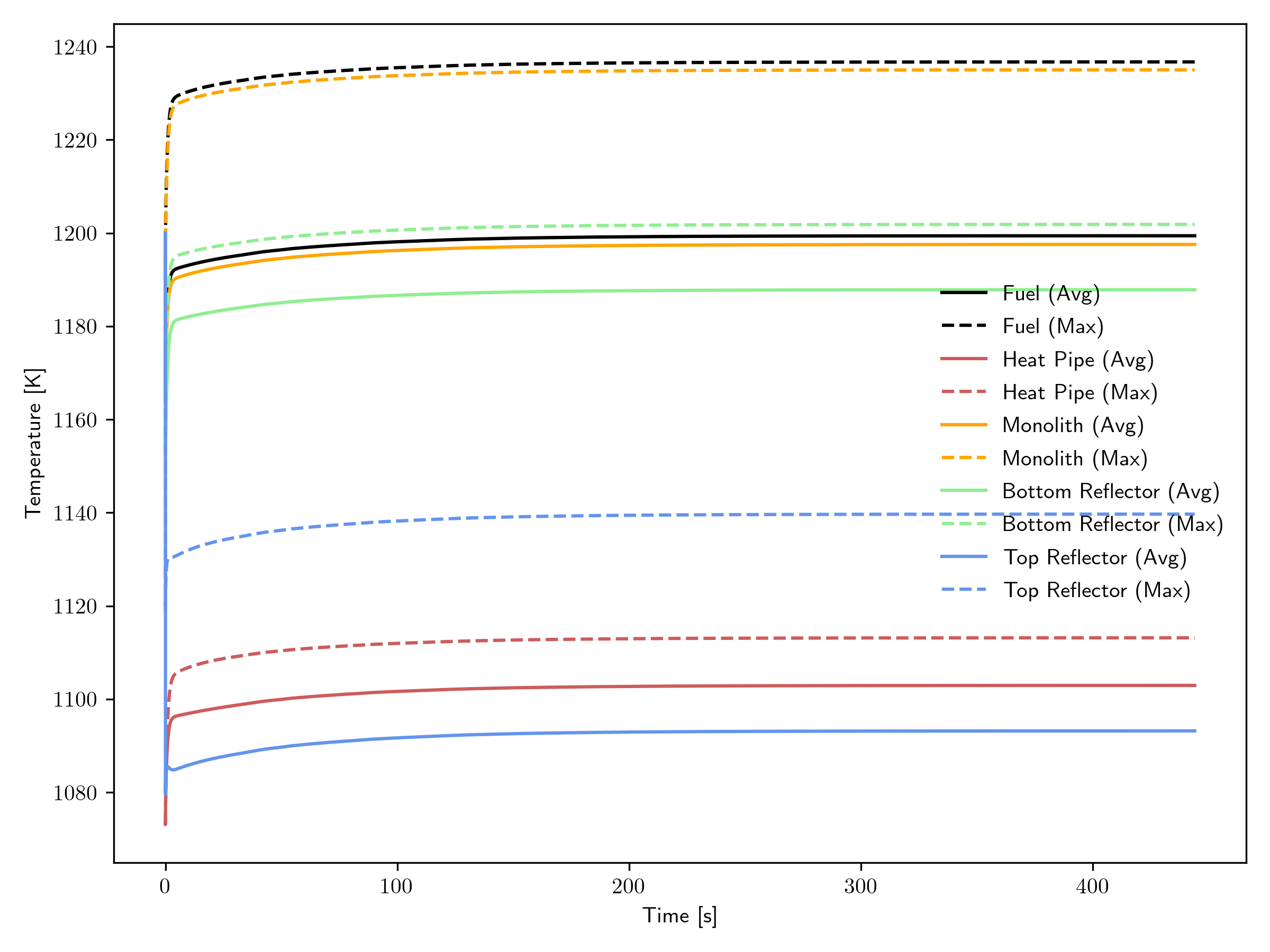
Figure 2: Transient of various temperatures.
Figure 3 gives the steady temperature distribution of each of the 7 heat pipes, both at the centerline and at the outer surface of the cladding. The heat pipe with index 3 corresponds to the central heat pipe, and as expected, has the lowest temperatures, since it is responsible for removing one third of the heat of the each of the surrounding 6 fuel pins (a total of 2 pins' heat), whereas each peripheral heat pipe is responsible for removing the heat of one third of each of 2 fuel pins, one half of each of 2 fuel pins, and two whole fuel pins, totaling the heat of 3 2/3 pins. The temperature drop over the length of each heat pipe is not negligible, roughly 15 K, which possibly invalidates the usage of simplified heat pipe models that assume perfectly isothermal operation. Also note there is a significant temperature drop across the cladding and liquid of the heat pipe, above 15 K, so this must also be taken into account.
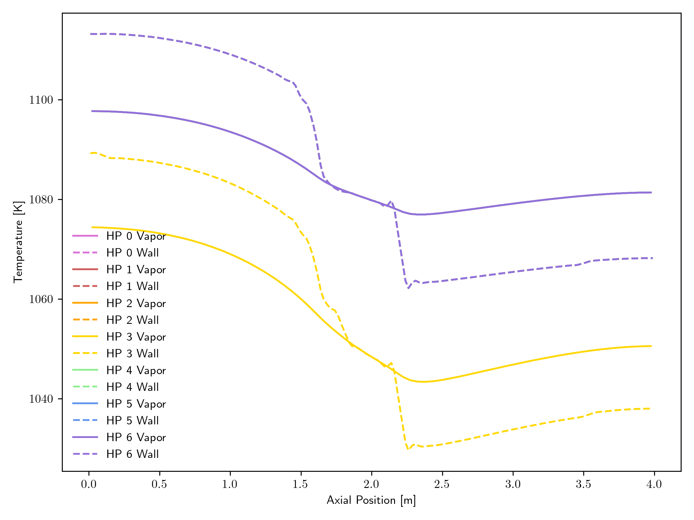
Figure 3: Steady heat pipe temperature distributions.
References
- N. Stauff, K. Mo, Y. Cao, J. Thomas, Y. Miao, L. Zou, D. Nunez, E. Shemon, B. Feng, and K. Ni.
Detailed analyses of a TRISO-fueled microreactor.
Technical Report ANL/NEAMS-21/3, Argonne National Laboratory, 2021.[BibTeX]