Cardinal Model of a 7-Pin Lead-cooled Fast Reactor (LFR) Assembly
Contact: Hansol Park, [email protected]
Model was co-developed by Yiqi Yu, Emily Shemon, and it was documented and uploaded by Jun Fang
Model link: 7-Pin Cardinal Model
This tutorial documents the development of a Cardinal multiphysics model aimed at predicting "hot channel factors" (HCF) in fast reactor designs (Shemon et al., 2018). The model utilizes Griffin (Lee et al., 2021), MOOSE (Lindsay et al., 2022), and NekRS (Fischer et al., 2022). HCFs are computed values that consider the impact of uncertainties in material properties, reactor geometry, and modeling approximations on predicted peak fuel, cladding, and coolant temperatures in the as-built reactor. Simplified geometry or physics in modeling approximations may lead to an overestimation of hot channel factors, resulting in unnecessarily conservative thermal design margins. Advanced modeling techniques could potentially reduce computed HCF values by addressing sources of modeling uncertainty, offering economic benefits for reactor vendors.
For high fidelity modeling, the reactor physics code Griffin (Lee et al., 2021) performs a fully heterogeneous fine-mesh transport calculation using the discontinuous finite element method with discrete ordinates (DFEM-) solver with Coarse Mesh Finite Difference (CMFD) acceleration, and the thermal hydraulics code NekRS (Fischer et al., 2022) performs the computational fluid dynamics (CFD) calculation. These codes were individually assessed in prior work to ensure the necessary capabilities were in place (Shemon et al., 2021). This work describes initial efforts to couple the codes using the MultiApp system of the MOOSE framework (Lindsay et al., 2022). The open-source MOOSE-wrapper for NekRS, Cardinal (Novak et al., 2022), is used to bring NekRS into the MOOSE coupled ecosystem for fluid temperature calculations, and the open source MOOSE heat transfer (H.T.) module is leveraged to perform solid temperature calculations.
Problem Specification
Due to the current lack of data on hot channel factors in lead-cooled fast reactors (LFR), a small 7-pin ducted LFR “mini-assembly” was developed as a proof-of-concept demonstration. The mini-assembly is based on a 127-pin ducted LFR assembly prototype (Shemon et al., 2021; Grasso et al., 2019) and is shown in Figure 1. The fuel rod geometry was adopted from the full assembly except there is no helium gap between the annular fuel and the cladding. Pin pitch, duct thickness, and height of the active fuel rod were adopted as-is. Cylindrical solid clad reflectors of length 20 cm and with the same diameter as the fuel rod are attached to the top and bottom of the fuel rod to mimic the realistic core configuration. For simplicity, the lead coolant inlet velocity was reduced from the original value of 1 m/s to 11.86 cm/s to keep the flow in the laminar regime (Reynolds number of 780), which can significantly reduce the runtime required for CFD. Accordingly, the total power was reduced by a factor of seven to bound the coolant temperature increase (~less than 300 K). However, we did not adjust the thermal conductivity of the solid materials, so the solid temperature range from fuel centerline to outer cladding surface is lower than in the prototypical concept. The coolant density is represented as a linear function of temperature for the coolant density reactivity feedback effect in neutronics calculation. MOOSE’s heat transfer module solves for solid temperature in all regions except the coolant.
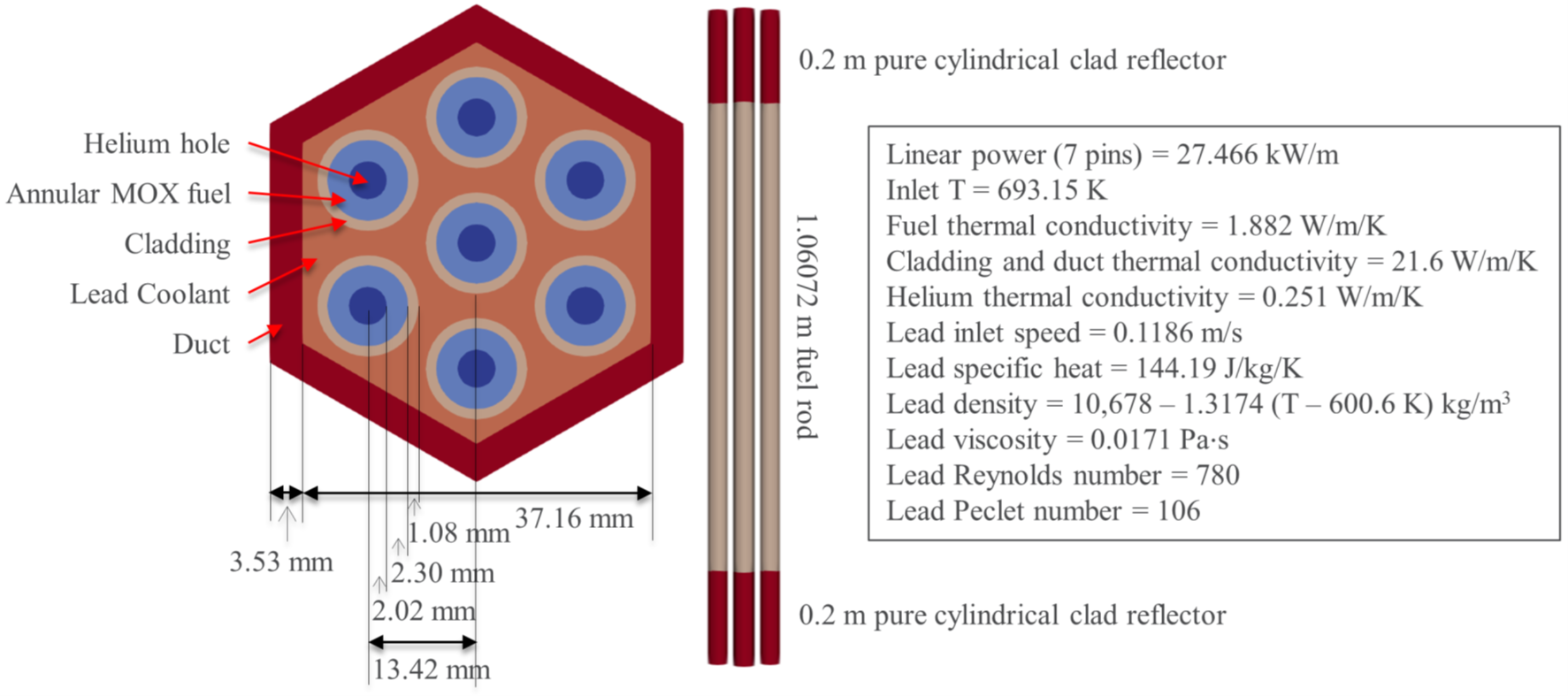
Figure 1: Problem specification of seven pins with duct (no inter-assembly gap).
Multiphysics Coupling
There are various numerical techniques to couple different physics. The Jacobian-Free Newton-Krylov (JFNK) method incorporates different physics variables in the system matrix and solves for all variables simultaneously. This is suitable for strongly coupled problems. However, this is not possible using the specific combination of three solvers in this work. Instead, the MOOSE MultiApp system provides an alternative method using Picard iterations and the operator splitting method.
MOOSE MultiApp hierarchy
When performing multiphysics simulations using the MOOSE MultiApp system (Lindsay et al., 2022), individual applications (physics solvers) are placed into a user-defined coupling hierarchy that determines when each solver is called and when data transfers occur. The “main” application sits at the top of the hierarchy and drives the simulation by calling “sub-applications” which sit below it. Subapplications can also drive their own sub-applications. The time step size of a sub-application cannot be bigger than that of the application above it. This rule requires NekRS to be placed at the lowest level (because NekRS uses the smallest time step size, due to constraints on the Courant Friedrichs-Lewy (CFL) number). Since NekRS and MOOSE H.T. solutions are tightly coupled through conjugate heat transfer, they are directly connected by H.T. calling NekRS as a subapplication. The Griffin neutronics solve is placed at the top of the hierarchy since it does not need to be called as frequently as the H.T. solve.
The detailed coupling scheme is shown in Figure 2. The conjugate heat transfer calculation between H.T. and NekRS is performed using the operator splitting method. H.T. proceeds for one time step, and then the heat fluxes at the solid-fluid (clad-coolant and duct-coolant) interfaces are transferred to NekRS for use as Neumann boundary conditions. Then, multiple NekRS time steps are solved using the sub_cycling option, and wall temperatures at the same interfaces are transferred back to H.T. for use as Dirichlet boundary conditions. Picard iteration is essentially achieved “in time”, so that running a large number of time steps is equivalent to converging to a pseudo-steady state. Note that the solid heat transfer solve does not have the time derivative term in the equation but is driven by the time dependent boundary condition in its Transient executioner, while NekRS solves the time-dependent Navier-Stokes equations.
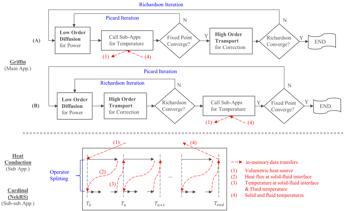
Figure 2: MOOSE MultiApp hierarchy for multiphysics coupling: (A) and (B) are both candidate choices for multiphysics coupling in the DFEM-/CMFD solver of Griffin.
The coupled MOOSE heat transfer and NekRS system is plugged under the MultiApp system of Griffin. Griffin solves a steady state eigenvalue problem and performs a Picard iteration with its sub-apps. The Griffin DFEM-/CMFD solver has the option to call sub-applications either inside or outside the Richardson iteration loop (controlled by the fixed_point_solve_outer parameter in the SweepUpdate executioner part of the input file). The calling of HT/NekRS from inside and outside the Richardson iteration loop are shown in (A) and (B) in Figure 2, respectively (Wang et al., 2021). In (A), temperature field is updated iteratively with the low order diffusion (CMFD) solution until temperature is converged, and once the temperature is converged, the high order transport (DFEM-) calculation is performed to update the closure term to be used in the diffusion calculation. The whole simulation is terminated once the neutron angular flux solution is converged. In (B), the neutronics and temperature calculations are separated; the temperature calculation is invoked every time the DFEM-/CMFD solution is converged. (B) was chosen in this work for the following reason. In (A), a partially converged power distribution is used to drive a fully converged CFD calculation for each neutronics Richardson iteration. This is computationally inefficient as CFD is very expensive and has to be performed with each Richardson iteration. In (B), the neutronics is allowed to converge first (it is not highly dependent on temperature), which then drives the CFD calculation. (B) is more computationally efficient for weakly coupled problems and also ensures convergence of the temperature distribution.
Data transfer
Figure 3 shows the data transfer scheme between different physics solvers. For transferring volumetric heat source from Griffin to H.T., Griffin computes constant volumetric heat source per element and the value at the centroid of an element in the H.T. mesh is queried from the finite element solution in the Griffin mesh and used as a constant value over the element (see MultiAppShapeEvaluationTransfer (Lindsay et al., 2022)). The transferred heat source is normalized to preserve the original total power using MOOSE’s conservative transfer features. For transferring the temperature field from H.T. to Griffin for Doppler and coolant density feedback, temperature values at the three closest nodes in the H.T. mesh to the target node in the Griffin mesh are interpolated using inverse distance weighting (see MultiAppGeometricInterpolationTransfer (Lindsay et al., 2022)). Nearest points are searched only in the solid region for solid temperatures and in the fluid region for fluid temperatures. Even though H.T. does not need the fluid domain for solving the heat conduction equation, the H.T. problem contains a mesh for the fluid domain in order to receive the coolant temperature field transferred from Cardinal (on its way to Griffin) and compute its L2-norm for convergence check. Note that Griffin does not need a fine mesh in the coolant region for neutronics solution, and a fine coolant mesh in H.T. does not degrade computational efficiency except in memory-limited cases.
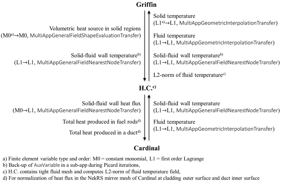
Figure 3: Data transfer scheme among Griffin, H.T., and Cardinal.
For the conjugate heat transfer, H.T. computes constant monomial heat flux per element at the cladding outer surfaces and the duct inner surface. Note that the heat flux variable computed by H.T. is of an elemental type (monomial), while the variable automatically added by Cardinal on the mirror mesh of the NekRS native mesh, is using a nodal type (lagrange). If there are multiple nearest centroids near parallel process boundaries or the nearest-nodes to the currently-considered centroids are not detected within the process boundary, parallel resolution between nearly equi-distant points may be inaccurate unless extensive searches are done over every process or a bounding box, for setting the search region in a heuristic, larger than the mesh discretization (the distance between the nodes and centroids that should be matched) is set in transfer. Due to this issue, a new nodal type heat flux is used for transfer by converting the elemental type variable to the nodal type using ProjectionAux before transfer. For the transfer, MultiAppGeneralFieldNearestLocationTransfer (Lindsay et al., 2022) is used separately for different interfaces (e.g. duct-coolant and clad-coolant) with spatial restrictions on source and target boundaries for the search. To preserve the total energy, the total power produced in the fuel rods and in the duct are separately transferred to Cardinal for normalization of the transferred heat flux at each interface by Cardinal. The heat flux could have been preserved on a per-rod basis but we chose not to because heat flux distribution among different fuel pins was calculated fairly accurately.
The solid-fluid wall temperature is transferred from Cardinal to H.T. in the same manner as the transfer of the heat flux.
Since the wall temperature is a part of the AuxiliarySystem in H.T. which is not restored during the Picard iteration even with keep_solution_during_restore = true (until this is issue in MOOSE is resolved) in FullSolveMultiApp, it is backed up via Griffin using the same transfer from Cardinal to H.T. Otherwise, the boundary condition in H.T. would be re-set per Picard iteration. The fluid temperature is transferred from Cardinal to H.T. in the same manner as the transfer from H.T. to Griffin.
Doppler and Coolant Density Reactivity Feedbacks
For the Doppler feedback, 9-group cross sections of each material are tabulated at two to three temperatures and linearly interpolated at the target temperature of each spatial quadrature point in an element. The detailed cross section generation procedure can be found in the LFR Single Assembly Model. For the coolant density feedback, the AuxVariable for the temperature dependent fluid density in Figure 1 is evaluated using the ParsedAux AuxKernel that uses the coupled variable for the coolant temperature in its expression. This fluid density AuxVariable is coupled to MultigroupTransportMaterial of Griffin for adjusting atomic density of the coolant material at each quadrature point in an element.
Convergence tolerance
For the scheme (B) in Figure 2, there are two convergence control parameters: the tolerances on the Richardson and Picard iterations. The Richardson iteration exits once drops down below (richardson_rel_tol = 1E-3) where is the neutron angular flux field at Richardson iteration. is a loose criterion but sufficient because the root-mean-square value of power distribution errors drops down below 0.01% at the relative Richardson error of in a non-coupled calculation. To exit the Picard iteration (end the whole simulation), the tolerance on the relative difference of the L2-norm of temperature field values computed by H.T. between successive Picard iterations was set as .
Computational strategy
The calculation procedure consists of two steps focused first on generating good initial conditions and then performing the full multiphysics run. First, a NekRS standalone calculation was performed to provide reasonable initial temperature, velocity, and pressure conditions. For this calculation, a crude heat flux distribution was obtained from Griffin where the inlet temperature condition was assigned uniformly to all regions. The dimensionless NekRS time step size of (0.09106 ms, after dimensionalization) was used to keep the Courant number less than 0.3. The simulation was run for 9.106 s, which is 75% of the time required for the flow to pass through from inlet to outlet.
As the flow is developed, the fully coupled simulation can freeze the velocity to speed up the development of the temperature. During the coupled simulation, the dimensionless NekRS time step size was increased by 10x (0.9106 ms) since the velocity was frozen. The H.T. solve was called every 50 NekRS time steps. Insufficiently frequent calls of H.T. cause instability in the solution (discussed in Results section). One hundred time steps were taken in H.T. per Picard iteration, so Griffin was called every 4.553 s, leading to the 5000:100:1 ratio of the number of NekRS, H.T., and Griffin calculations.
Griffin Input Model
This section decribes the input file for Griffin using the DFEM- solver with the CMFD acceleration.
Input parameters
Defining input parameters in advance is beneficial to make the input tractable because the same value can be used in multiple places. Block IDs and material IDs to be assigned to block IDs and the total power are defined as input parameters to be used in the main input later.
activefuelheight = 1.06072      # m
#lowerreflectorheight = 0.2      # m
#upperreflectorheight = 0.2      # m

#num_coolreg = 2
#num_coolreg_back = 2
num_layers_fuel = 20
num_layers_refl = 4
#numside=6

linearpower = 27466.11572112955 # W/m
inlet_T = 693.15                # K
fuelconductance = 1.882        # W/m/K
#cladconductance = 21.6         # W/m/K

mid_gap = 1
mid_ifl = 2
mid_ofl = 3
mid_clad = 4
mid_cool = 5
mid_duct = 6

# === derived
#half_asmpitch = ${fparse flat_to_flat / 2 + duct_thickness}
coolantdensity_ref = ${fparse 10678 - 13174 * (inlet_T - 600.6) / 10000} # kg/m^3

richardsonreltol=1E-1
richardsonabstol=1E+5
maxinnerits=1
maxfixptits=100000
richardsonmaxits=1000Meshes for Griffin, heat transfer and Cardinal solvers
The Griffin and H.T. meshes were generated with the MOOSE Reactor module (Shemon et al., 2022) which allows for mesh perturbation using the MOOSE Stochastic Tools in the future. The Cardinal mesh is the mirror mesh of the NekRS native mesh and is built by Cardinal automatically by looping through the CFD mesh and copying elements into a lower-order representation. Attention was paid to keeping the azimuthal division in the Griffin and H.T. meshes similar to that in the Cardinal mesh for better alignment of nodes on the cladding outer surfaces and duct inner surfaces among the different meshes. Each duct side was divided into 18 segments in all meshes. H.T. has a finer mesh radially and axially than Griffin: 23 vs. 6 in a fuel rod, 10 vs. 2 in a duct, and 16 vs. 4 in a coolant in the radial direction and 48 vs. 24 in the axial direction. In H.T., fine meshes in the fuel rod and the duct are needed for accurate temperature and heat flux calculations. The finer meshes in the coolant region are used for better convergence metric of the coolant temperature, and those in the axial direction are used for better NearestNode data transfer of heat flux and surface temperature between H.T. and Cardinal. The Cardinal (NekRS) axial mesh is finer in the inlet region to accurately compute the entrance effect. The overall mesh configurations for each individual physics solver can be found in Figure 4.
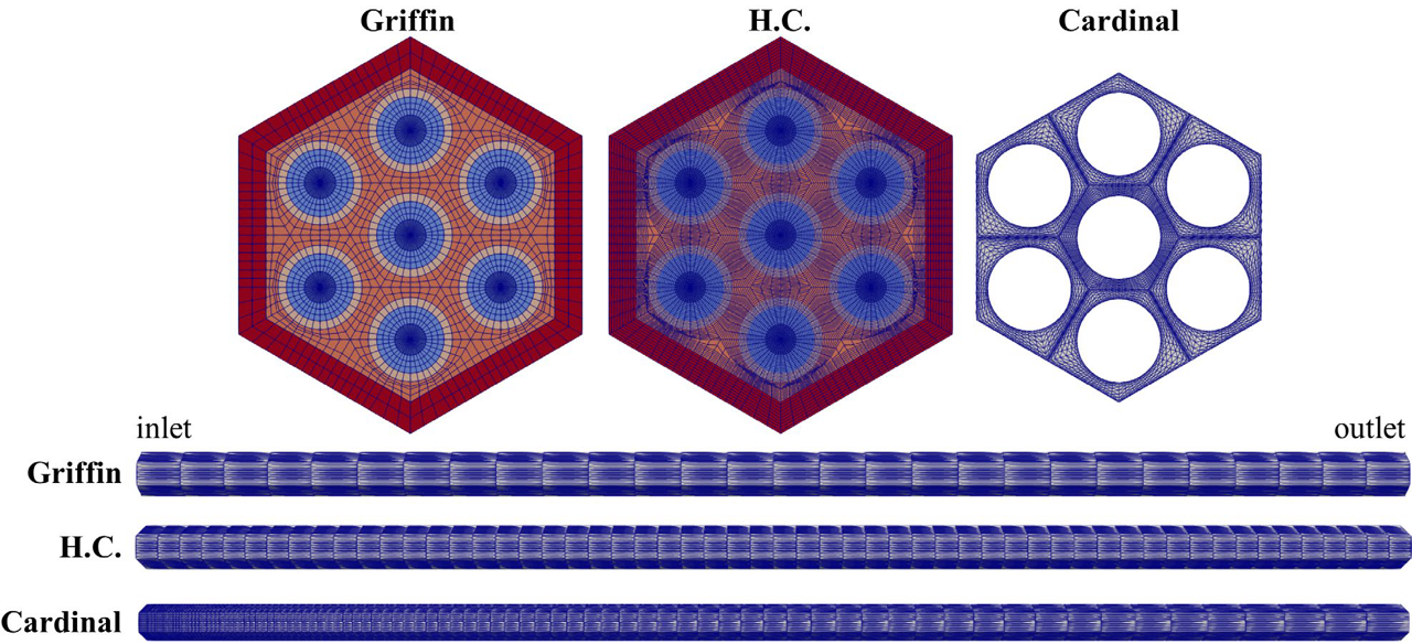
Figure 4: Radial (top) and axial (bottom) meshes of Griffin, H.T., and Cardinal.
In the Griffin input file, we can load the mesh files produced by MOOSE Reactor module as follows
[Mesh]
  [fmg]
    type = FileMeshGenerator
    file = 'NTmesh_in.e'
    exodus_extra_element_integers = 'material_id pin_id coarse_element_id'
  []
[]Please note that the Griffin mesh provided is already in Exodus format, created using the MOOSE mesh module and the input file NTmesh.i. Users can generate this mesh using NTmesh.i with griffin-opt or any other MOOSE application including the Reactor module:
griffin-opt -i NTmesh.i --mesh-only
The heat transfer mesh can be generated in the similar way using the input file HCmesh.i provided.
griffin-opt -i HCmesh.i --mesh-only
Executioner
The SweepUpdate executioner is used for the CMFD acceleration. SweepUpdate is a special Richardson executioner for performing source iteration with a transport sweeper. This source iteration can be accelerated by turning on cmfd_acceleration which invokes the CMFD solve where the low order diffusion equation is solved with a convection closure term to make the diffusion system and the transport system consistent. richardson_rel_tol or richardson_abs_tol is the tolerance used to check the convergence of the Richardson iteration. richardson_max_its is the maximum number of iterations allowed for Richardson iterations. These parameters are controlled by the corresponding variables given in Input parameters. If richardson_postprocessor is specified, its PostProcessor value is used as the convergence metric. Otherwise Griffin uses the L2 norm difference of the angular flux solution between successive Richardson iterations, which is added to richardson_postprocessor with the name of flux_error internally. richardson_rel_tol is the tolerance for the ratio of the richardson_postprocessor value of the current iteration to that of the first iteration. richardson_value is for the console output purpose to show the history of PostProcessor values over Richardson iterations, and it is set to be eigenvalue. inner_solve_type is about the way to perform the inner solve of the Richardson iteration. There are three options: none, SI and GMRes. none is just a direct transport operator inversion per residual evaluation, while scattering source is updated together for SI and GMRes per residual evaluation. The latter two options involve more number of transport sweeps per residual evaluation than none, leading to the reduction of the number of residual evaluations and possibly the total run time. For GMRes, the scattering source effect is accounted for at once by performing the GMRes iterations and max_inner_its is the maximum number of GMRes iterations. For SI, the scattering source effect is accounted for by performing source iterations and max_inner_its is the maximum number of source iterations.
fixed_point_solve_outer is configured to allow Griffin to invoke the Picard iteration between Griffin and its sub-app (H.T. and nekRS) calculations outside the Richardson iteration. This approach has been demonstrated to be more computationally efficient for weakly coupled problems in the multiphysics hierarchy. The convergence criterion is based on the temperature field with a relative tolerance custom_rel_tol of 1e-5.
coarse_element_id is the name of the extra element integer ID assigned in the mesh file. If the CMFD solve does not converge, one can try different options for diffusion_eigen_solver_type which is the eigenvalue solver for CMFD. There are four options: power, arnoldi, krylovshur and newton. newton is the default which is recommended to stick with. If newton does not converge a solution, either krylovshur is the second option to go with, or cmfd_prec_type can be changed to lu from its default value of boomeramg for a small problem. Also one can try cmfd_closure_type=syw or cmfd_closure_type=pcmfd as different ways, but it is recommended to stick with its default value of traditional_cmfd.
[Executioner]
  type = SweepUpdate
  verbose = false

  richardson_rel_tol = ${richardsonreltol}
  richardson_abs_tol = ${richardsonabstol}
  richardson_max_its = ${richardsonmaxits}
  richardson_value = 'eigenvalue'
  inner_solve_type = GMRes
  max_inner_its = ${maxinnerits}

  fixed_point_solve_outer = true
  fixed_point_max_its = ${maxfixptits}
  custom_pp = nek_bulk_temp_pp
  custom_rel_tol = 1e-8
  force_fixed_point_solve = true

  cmfd_acceleration = true
  coarse_element_id = coarse_element_id
  diffusion_eigen_solver_type = newton
  prolongation_type = multiplicative
[]Power Density
Within this segment, the variable power represents the total power specified by the user, and power_density_variable is a mandatory AuxVariable name for power density. The evaluation of power density is conducted using the normalized neutronics solution.
[PowerDensity]
  power = ${fparse linearpower * activefuelheight} # W
  power_density_variable = power_density
  integrated_power_postprocessor = integrated_power
  power_scaling_postprocessor = power_scaling
  family = MONOMIAL
  order = CONSTANT
[]Transport systems
For the transport system, particle is neutron and equation_type is eigenvalue. The number of energy groups is 9 given by G and VacuumBoundary and ReflectingBoundary are sideset names: top and bottom surfaces are vacuum and lateral surfaces are reflective. In the sub-block of [sn], the DFEM-SN scheme is specified. Between monomial and L2-Lagrange families of basis functions supported for discontinuous elements, the monomial type is selected with the first order. The angular quadrature type (AQtype) is set to Gauss-Chebyshev for having a freedom to choose a different number of angles in the azimuthal direction and in the polar direction in 3D. The number of azimuthal angles (NAzmthl) and that of polar angles (NPolar) per octant are set to and , respectively, from a sensitivity study. The anisotropic scattering order (NA) is set to 1. using_array_variable=true and collapse_scattering=true are recommended options for performance reason in general.
[TransportSystems]
  particle = neutron
  equation_type = eigenvalue
  G = 9
  ReflectingBoundary = 'ASSEMBLY_SIDE'
  VacuumBoundary = 'ASSEMBLY_TOP ASSEMBLY_BOTTOM'
  [sn]
    scheme = DFEM-SN
    family = MONOMIAL
    order = FIRST
    AQtype = Gauss-Chebyshev
    NPolar = 2
    NAzmthl = 3
    NA = 1
    sweep_type = asynchronous_parallel_sweeper
    using_array_variable = true
    collapse_scattering  = true
  []
AuxVariables
The AuxVariables block is specified next. Through the Auxiliary Variables, developers can define external variables that are solved or used in the Griffin simulation. Specifically, the additional variables defined include the solid temperature solid_temp, the fluid density fluid_density, the solid-fluid surface temperature nek_surf_temp, and the fluid bulk temperature nek_bulk_temp sourced from nekRS.
[AuxVariables]
  [nek_bulk_temp]
    block = 'Lead'
    initial_condition = ${inlet_T}  # K
  []
  [solid_temp]
    block = 'HeliumHolePrism HeliumHole Clad Fuel00 Fuel10 Fuel11 Fuel12 Fuel13 Fuel14 Fuel15 LowerHeliumHolePrism LowerHeliumHole LowerClad LowerFuel00 LowerFuel10 LowerFuel11 LowerFuel12 LowerFuel13 LowerFuel14 LowerFuel15 UpperHeliumHolePrism UpperHeliumHole UpperClad UpperFuel00 UpperFuel10 UpperFuel11 UpperFuel12 UpperFuel13 UpperFuel14 UpperFuel15 Duct'
    initial_condition = ${inlet_T} # K
  []
  [fluid_density]
    block = 'Lead'
    initial_condition = ${coolantdensity_ref}  # kg/m^3
  []
  [nek_surf_temp]
    initial_condition = ${inlet_T}  # K
  []
[]AuxKernels
The AuxKernels is set up to update the fluid density based on the fluid temperature obtained from NekRS.
[AuxKernels]
  [fluid_density_temp]
    type = ParsedAux
    variable = fluid_density
    coupled_variables = 'nek_bulk_temp'
    expression = '10678-13174*(nek_bulk_temp-600.6)/10000'
    execute_on = 'INITIAL timestep_end'
  []
[]GlobalParams
In [GlobalParams], is_meter=true is to indicate that the mesh is in a unit of meter and plus=true to indicate that absorption, fission, and kappa fission cross sections are to be evaluated.
[GlobalParams]
    plus = true
    dbgmat = false
    grid_names = 'Temp'
    maximum_diffusion_coefficient = 1000
    is_meter = true
[]Compositions
The [Compositions] block is employed to define the compositions of the six materials considered in the Griffin model. composition_ids serves as material_id that has been already assigned in the mesh generation stage.
[Compositions]
  [IF_HELIUM00]
    type = IsotopeComposition
    isotope_densities = 'pseudo_HE4__FR1 2.512611E-05'
    density_type = atomic
    composition_ids = ${mid_gap}
  []
  [IF_FUELR100]
    type = IsotopeComposition
    isotope_densities = 'pseudo_U234_FR1 1.769055E-07
                         pseudo_U235_FR1 4.404137E-05
                         pseudo_U238_FR1 1.735054E-02
                         pseudo_PU238FR1 1.244939E-05
                         pseudo_PU239FR1 3.413306E-03
                         pseudo_PU240FR1 1.319941E-03
                         pseudo_PU241FR1 8.656869E-05
                         pseudo_PU242FR1 1.234538E-04
                         pseudo_AM241FR1 2.087265E-04
                         pseudo_O16__FR1 4.444138E-02'
    density_type = atomic
    composition_ids = ${mid_ifl}
  []
  [IF_FUELR200]
    type = IsotopeComposition
    isotope_densities = 'pseudo_U234_FR2 1.769055E-07
                         pseudo_U235_FR2 4.404137E-05
                         pseudo_U238_FR2 1.735054E-02
                         pseudo_PU238FR2 1.244939E-05
                         pseudo_PU239FR2 3.413306E-03
                         pseudo_PU240FR2 1.319941E-03
                         pseudo_PU241FR2 8.656869E-05
                         pseudo_PU242FR2 1.234538E-04
                         pseudo_AM241FR2 2.087265E-04
                         pseudo_O16__FR2 4.444138E-02'
    density_type = atomic
    composition_ids = ${mid_ofl}
  []
  [IF_CLAD00]
    type = IsotopeComposition
    isotope_densities = 'pseudo_FE54_FCD 3.185952E-03
                         pseudo_FE56_FCD 5.001168E-02
                         pseudo_FE57_FCD 1.154947E-03
                         pseudo_FE58_FCD 1.537129E-04
                         pseudo_NI58_FCD 8.373412E-03
                         pseudo_NI60_FCD 3.225451E-03
                         pseudo_NI61_FCD 1.402235E-04
                         pseudo_NI62_FCD 4.469793E-04
                         pseudo_NI64_FCD 1.138947E-04
                         pseudo_CR50_FCD 5.643439E-04
                         pseudo_CR52_FCD 1.088250E-02
                         pseudo_CR53_FCD 1.234043E-03
                         pseudo_CR54_FCD 3.071758E-04
                         pseudo_MN55_FCD 1.271641E-03
                         pseudo_MO92_FCD 1.080550E-04
                         pseudo_MO94_FCD 6.735188E-05
                         pseudo_MO95_FCD 1.159146E-04
                         pseudo_MO96_FCD 1.214544E-04
                         pseudo_MO97_FCD 6.953578E-05
                         pseudo_MO98_FCD 1.757019E-04
                         pseudo_MO100FCD 7.011875E-05
                         pseudo_SI28_FCD 1.300140E-03
                         pseudo_SI29_FCD 6.601594E-05
                         pseudo_SI30_FCD 4.351798E-05
                         pseudo_C____FCD 3.489938E-04
                         pseudo_P31__FCD 6.766687E-05
                         pseudo_S32__FCD 2.068704E-05
                         pseudo_S33__FCD 1.656123E-07
                         pseudo_S34__FCD 9.348567E-07
                         pseudo_S36__FCD 4.358298E-09
                         pseudo_TI46_FCD 3.210951E-05
                         pseudo_TI47_FCD 2.895766E-05
                         pseudo_TI48_FCD 2.869267E-04
                         pseudo_TI49_FCD 2.105602E-05
                         pseudo_TI50_FCD 2.016107E-05
                         pseudo_V____FCD 2.742873E-05
                         pseudo_ZR90_FCD 7.880535E-06
                         pseudo_ZR91_FCD 1.718520E-06
                         pseudo_ZR92_FCD 2.626878E-06
                         pseudo_ZR94_FCD 2.662077E-06
                         pseudo_ZR96_FCD 4.288701E-07
                         pseudo_W182_FCD 2.014107E-06
                         pseudo_W183_FCD 1.087650E-06
                         pseudo_W184_FCD 2.337892E-06
                         pseudo_W186_FCD 2.160800E-06
                         pseudo_CU63_FCD 1.520930E-05
                         pseudo_CU65_FCD 6.778986E-06
                         pseudo_CO59_FCD 2.370990E-05
                         pseudo_CA40_FCD 3.379743E-05
                         pseudo_CA42_FCD 2.255696E-07
                         pseudo_CA43_FCD 4.706582E-08
                         pseudo_CA44_FCD 7.272563E-07
                         pseudo_CA46_FCD 1.394535E-09
                         pseudo_CA48_FCD 6.519498E-08
                         pseudo_NB93_FCD 7.519752E-06
                         pseudo_N14__FCD 4.969370E-05
                         pseudo_N15__FCD 1.835515E-07
                         pseudo_AL27_FCD 2.589280E-05
                         pseudo_TA181FCD 3.861021E-06
                         pseudo_B10__FCD 5.144462E-06
                         pseudo_B11__FCD 2.070704E-05'
    density_type = atomic
    composition_ids = ${mid_clad}
  []
  [IF_WRAPPER00]
    type = IsotopeComposition
    isotope_densities = 'pseudo_FE54_FWR 3.192503E-03
                         pseudo_FE56_FWR 5.011505E-02
                         pseudo_FE57_FWR 1.157401E-03
                         pseudo_FE58_FWR 1.540302E-04
                         pseudo_NI58_FWR 8.390808E-03
                         pseudo_NI60_FWR 3.232103E-03
                         pseudo_NI61_FWR 1.405101E-04
                         pseudo_NI62_FWR 4.479004E-04
                         pseudo_NI64_FWR 1.141301E-04
                         pseudo_CR50_FWR 5.655206E-04
                         pseudo_CR52_FWR 1.090501E-02
                         pseudo_CR53_FWR 1.236601E-03
                         pseudo_CR54_FWR 3.078103E-04
                         pseudo_MN55_FWR 1.274301E-03
                         pseudo_MO92_FWR 1.082801E-04
                         pseudo_MO94_FWR 6.749107E-05
                         pseudo_MO95_FWR 1.161601E-04
                         pseudo_MO96_FWR 1.217001E-04
                         pseudo_MO97_FWR 6.968007E-05
                         pseudo_MO98_FWR 1.760602E-04
                         pseudo_MO100FWR 7.026407E-05
                         pseudo_SI28_FWR 1.302801E-03
                         pseudo_SI29_FWR 6.615206E-05
                         pseudo_SI30_FWR 4.360804E-05
                         pseudo_C____FWR 3.497203E-04
                         pseudo_P31__FWR 6.780707E-05
                         pseudo_S32__FWR 2.073002E-05
                         pseudo_S33__FWR 1.659602E-07
                         pseudo_S34__FWR 9.367909E-07
                         pseudo_S36__FWR 4.367304E-09
                         pseudo_TI46_FWR 3.217603E-05
                         pseudo_TI47_FWR 2.901703E-05
                         pseudo_TI48_FWR 2.875203E-04
                         pseudo_TI49_FWR 2.110002E-05
                         pseudo_TI50_FWR 2.020302E-05
                         pseudo_V____FWR 2.748603E-05
                         pseudo_ZR90_FWR 7.896908E-06
                         pseudo_ZR91_FWR 1.722102E-06
                         pseudo_ZR92_FWR 2.632303E-06
                         pseudo_ZR94_FWR 2.667603E-06
                         pseudo_ZR96_FWR 4.297604E-07
                         pseudo_W182_FWR 2.018302E-06
                         pseudo_W183_FWR 1.089901E-06
                         pseudo_W184_FWR 2.342702E-06
                         pseudo_W186_FWR 2.165302E-06
                         pseudo_CU63_FWR 1.524101E-05
                         pseudo_CU65_FWR 6.793007E-06
                         pseudo_CO59_FWR 2.375902E-05
                         pseudo_CA40_FWR 3.386703E-05
                         pseudo_CA42_FWR 2.260402E-07
                         pseudo_CA43_FWR 4.716405E-08
                         pseudo_CA44_FWR 7.287707E-07
                         pseudo_CA46_FWR 1.397401E-09
                         pseudo_CA48_FWR 6.533006E-08
                         pseudo_NB93_FWR 7.535407E-06
                         pseudo_N14__FWR 4.979705E-05
                         pseudo_N15__FWR 1.839302E-07
                         pseudo_AL27_FWR 2.594703E-05
                         pseudo_TA181FWR 3.869004E-06
                         pseudo_B10__FWR 5.155105E-06
                         pseudo_B11__FWR 2.075002E-05'
    density_type = atomic
    composition_ids = ${mid_duct}
  []
  [IF_LEADCOOL00]
    type = IsotopeComposition
    isotope_densities = 'pseudo_PB204FCO ${fparse 4.232323E-04*coolantdensity_ref/10401.99540132}
                         pseudo_PB206FCO ${fparse 7.285612E-03*coolantdensity_ref/10401.99540132}
                         pseudo_PB207FCO ${fparse 6.680995E-03*coolantdensity_ref/10401.99540132}
                         pseudo_PB208FCO ${fparse 1.584046E-02*coolantdensity_ref/10401.99540132}'
    density_type = atomic
    composition_ids = ${mid_cool}
    fluid_density = fluid_density
    reference_fluid_density = ${coolantdensity_ref}
  []
[]Materials
The [Materials] block is constructed using MicroNeutronicsMaterial. This neutronics material loads a multigroup library with tabulated microscopic group cross sections of isotopes in ISOXML format. It evaluates macroscopic group cross sections with multiple material IDs based on the inputted isotope densities. The main reason for using this material instead of MixedNeutronicsMaterial is that each library (library ID) in the library file is not generated for each material (material ID) in the Griffin transport calculation. Using MicroNeutronicsMaterial, different material IDs can be freely generated in the same library ID.
Library ID refers to the value of the attribute named ID of the Multigroup_Cross_Section_Library element in the isoxml file. One should make sure that isotope names in the composition of a material_id covered by each MicroNeutronicsMaterial exist under the Multigroup_Cross_Section_Library with the ID specified by library_id in the isoxml file. grid_variables is the coupled variable used for temperature interpolation of cross sections for the Doppler feedback. For the coolant density feedback, a domain is recognized as fluid by fluid_density and reference_fluid_density input parameters and the macroscopic cross section of the region is scaled by the ratio of the value of the coupled variable fluid_density to the reference density per element quadrature. One caveat is that library_file and library_name common for all MicroNeutronicsMaterials should not be taken out to [GlobalParams] because the [MultiApps] block has the same input parameters meant for the dynamic library of sub-applications.
[Materials]
  [Neutronics_fuel_gap]
    type = MicroNeutronicsMaterial
    library_file = LFR9g_P5.xml
    library_name = ISOTXS-neutron
    library_id = 3
    block = 'HeliumHolePrism HeliumHole Fuel00 Fuel10 Fuel11 Fuel12 Fuel13 Fuel14 Fuel15'
    grid_variables = solid_temp
  []
  [Neutronics_clad_duct]
    type = MicroNeutronicsMaterial
    library_file = LFR9g_P5.xml
    library_name = ISOTXS-neutron
    library_id = 2
    block = 'Clad Duct LowerHeliumHolePrism LowerHeliumHole LowerClad LowerFuel00 LowerFuel10 LowerFuel11 LowerFuel12 LowerFuel13 LowerFuel14 LowerFuel15 UpperHeliumHolePrism UpperHeliumHole UpperClad UpperFuel00 UpperFuel10 UpperFuel11 UpperFuel12 UpperFuel13 UpperFuel14 UpperFuel15'
    grid_variables = solid_temp
  []
  [Neutronics_cool]
    type = MicroNeutronicsMaterial
    library_file = LFR9g_P5.xml
    library_name = ISOTXS-neutron
    library_id = 2
    block = 'Lead'
    grid_variables = nek_bulk_temp
  []
[]MultiApps and Transfers
[MultiApps] specifies how the Griffin model interacts with its sub-app HC.i, which is a MOOSE heat transfer model. Meanwhile, [Transfers] defines how the data is exchanged between Griffin model NT.i and the sub-app HC.i as illustrated in Figure 3.
[MultiApps]
  [HeatConduction]
    type = FullSolveMultiApp
    # To be replaced by the Application block
    # app_type = CardinalApp
    # library_path = '/projects/neams_ad_fr/testing_dl/cardinal/lib'
    input_files = HC.i
    keep_solution_during_restore = true
    execute_on = 'timestep_end'
    cli_args = 'Materials/HeatConduct_Fuel/thermal_conductivity=${fuelconductance}'
  []
[]

[Transfers]
  [PowerDensity_to_HeatConduction]
    type = MultiAppGeneralFieldShapeEvaluationTransfer
    to_multi_app = HeatConduction
    source_variable = power_density
    variable = heat_source
    from_postprocessors_to_be_preserved = power_density_pp
    to_postprocessors_to_be_preserved = heat_source_rod_duct
  []
  [solid_temp_from_HeatConduction]
    type = MultiAppGeometricInterpolationTransfer
    from_multi_app = HeatConduction
    source_variable = solid_temp
    variable = solid_temp
  []
  [nek_bulk_temp_from_nek]
    type = MultiAppGeometricInterpolationTransfer
    from_multi_app = HeatConduction
    source_variable = nek_bulk_temp
    variable = nek_bulk_temp
  []

  [nek_surf_temp_rod_from_HeatConduction]
    type = MultiAppGeneralFieldNearestLocationTransfer
    source_variable = nek_surf_temp
    variable = nek_surf_temp
    from_boundaries = 'ROD_SIDE'
    to_boundaries = 'ROD_SIDE'
    from_multi_app = HeatConduction
    search_value_conflicts = false
  []
  [nek_surf_temp_rod_to_HeatConduction]
    type = MultiAppGeneralFieldNearestLocationTransfer
    source_variable = nek_surf_temp
    variable = nek_surf_temp
    from_boundaries = 'ROD_SIDE'
    to_boundaries = 'ROD_SIDE'
    to_multi_app = HeatConduction
    search_value_conflicts = false
  []
  [nek_surf_temp_duct_from_HeatConduction]
    type = MultiAppGeneralFieldNearestLocationTransfer
    source_variable = nek_surf_temp
    variable = nek_surf_temp
    from_boundaries = 'DUCT_INNERSIDE'
    to_boundaries = 'DUCT_INNERSIDE'
    from_multi_app = HeatConduction
    search_value_conflicts = false
  []
  [nek_surf_temp_duct_to_HeatConduction]
    type = MultiAppGeneralFieldNearestLocationTransfer
    source_variable = nek_surf_temp
    variable = nek_surf_temp
    from_boundaries = 'DUCT_INNERSIDE'
    to_boundaries = 'DUCT_INNERSIDE'
    to_multi_app = HeatConduction
    search_value_conflicts = false
  []

  [nek_bulk_temp_pp]
    type = MultiAppPostprocessorTransfer
    to_postprocessor = nek_bulk_temp_pp
    from_postprocessor = nek_bulk_temp_pp
    from_multi_app = HeatConduction
    reduction_type = maximum
  []
[]UserObjects and Postprocessors
Both [Postprocessors] and [VectorPostprocessors] can be used to compute quantities of interest from the solution to be included in output or used by other MOOSE applications. With [UserObjects], the users can extract the layer averaged quantities of interested, such as the power density, solid temperature, etc.
[UserObjects]
  [power_axial_uo]
    type = LayeredAverage
    variable = power_density
    direction = z
    num_layers = ${fparse num_layers_refl + num_layers_fuel + num_layers_refl}
  []
  [powerl_axial_uo]
    type = LayeredAverage
    variable = power_density
    direction = z
    num_layers = ${fparse num_layers_refl + num_layers_fuel + num_layers_refl}
    block = 'Lead'
  []
  [powergap_axial_uo]
    type = LayeredAverage
    variable = power_density
    direction = z
    num_layers = ${fparse num_layers_refl + num_layers_fuel + num_layers_refl}
    block = 'HeliumHolePrism HeliumHole LowerHeliumHolePrism LowerHeliumHole UpperHeliumHolePrism UpperHeliumHole'
  []
  [powerclad_axial_uo]
    type = LayeredAverage
    variable = power_density
    direction = z
    num_layers = ${fparse num_layers_refl + num_layers_fuel + num_layers_refl}
    block = 'Clad LowerClad UpperClad'
  []
  [powerduct_axial_uo]
    type = LayeredAverage
    variable = power_density
    direction = z
   num_layers = ${fparse num_layers_refl + num_layers_fuel + num_layers_refl}
    block = 'Duct'
  []
  [powerif_axial_uo]
    type = LayeredAverage
    variable = power_density
    direction = z
    num_layers = ${fparse num_layers_refl + num_layers_fuel + num_layers_refl}
    block = 'Fuel00 LowerFuel00 UpperFuel00'
  []
  [powerof1_axial_uo]
    type = LayeredAverage
    variable = power_density
    direction = z
    num_layers = ${fparse num_layers_refl + num_layers_fuel + num_layers_refl}
    block = 'Fuel10 LowerFuel10 UpperFuel10'
  []
  [powerof2_axial_uo]
    type = LayeredAverage
    variable = power_density
    direction = z
    num_layers = ${fparse num_layers_refl + num_layers_fuel + num_layers_refl}
    block = 'Fuel11 LowerFuel11 UpperFuel11'
  []
  [powerof3_axial_uo]
    type = LayeredAverage
    variable = power_density
    direction = z
    num_layers = ${fparse num_layers_refl + num_layers_fuel + num_layers_refl}
    block = 'Fuel12 LowerFuel12 UpperFuel12'
  []
  [powerof4_axial_uo]
    type = LayeredAverage
    variable = power_density
    direction = z
    num_layers = ${fparse num_layers_refl + num_layers_fuel + num_layers_refl}
    block = 'Fuel13 LowerFuel13 UpperFuel13'
  []
  [powerof5_axial_uo]
    type = LayeredAverage
    variable = power_density
    direction = z
    num_layers = ${fparse num_layers_refl + num_layers_fuel + num_layers_refl}
    block = 'Fuel14 LowerFuel14 UpperFuel14'
  []
  [powerof6_axial_uo]
    type = LayeredAverage
    variable = power_density
    direction = z
    num_layers = ${fparse num_layers_refl + num_layers_fuel + num_layers_refl}
    block = 'Fuel15 LowerFuel15 UpperFuel15'
  []
  [fluidtemp_axial_uo]
    type = LayeredAverage
    variable = nek_bulk_temp
    direction = z
    num_layers = ${fparse num_layers_refl + num_layers_fuel + num_layers_refl}
    block = 'Lead'
  []
  [iftemp_axial_uo]
    type = LayeredAverage
    variable = solid_temp
    direction = z
    num_layers = ${fparse num_layers_refl + num_layers_fuel + num_layers_refl}
    block = 'Fuel00 LowerFuel00 UpperFuel00'
  []
  [of1temp_axial_uo]
    type = LayeredAverage
    variable = solid_temp
    direction = z
    num_layers = ${fparse num_layers_refl + num_layers_fuel + num_layers_refl}
    block = 'Fuel10 LowerFuel10 UpperFuel10'
  []
  [of2temp_axial_uo]
    type = LayeredAverage
    variable = solid_temp
    direction = z
    num_layers = ${fparse num_layers_refl + num_layers_fuel + num_layers_refl}
    block = 'Fuel11 LowerFuel11 UpperFuel11'
  []
  [of3temp_axial_uo]
    type = LayeredAverage
    variable = solid_temp
    direction = z
    num_layers = ${fparse num_layers_refl + num_layers_fuel + num_layers_refl}
    block = 'Fuel12 LowerFuel12 UpperFuel12'
  []
  [of4temp_axial_uo]
    type = LayeredAverage
    variable = solid_temp
    direction = z
    num_layers = ${fparse num_layers_refl + num_layers_fuel + num_layers_refl}
    block = 'Fuel13 LowerFuel13 UpperFuel13'
  []
  [of5temp_axial_uo]
    type = LayeredAverage
    variable = solid_temp
    direction = z
    num_layers = ${fparse num_layers_refl + num_layers_fuel + num_layers_refl}
    block = 'Fuel14 LowerFuel14 UpperFuel14'
  []
  [of6temp_axial_uo]
    type = LayeredAverage
    variable = solid_temp
    direction = z
    num_layers = ${fparse num_layers_refl + num_layers_fuel + num_layers_refl}
    block = 'Fuel15 LowerFuel15 UpperFuel15'
  []
  [cladtemp_axial_uo]
    type = LayeredAverage
    variable = solid_temp
    direction = z
    num_layers = ${fparse num_layers_refl + num_layers_fuel + num_layers_refl}
    block = 'Clad LowerClad UpperClad'
  []
  [ducttemp_axial_uo]
    type = LayeredAverage
    variable = solid_temp
    direction = z
    num_layers = ${fparse num_layers_refl + num_layers_fuel + num_layers_refl}
    block = 'Duct'
  []
[]

[Postprocessors]
  [nek_bulk_temp_pp]
    type = Receiver
  []
  [fluid_density]
    type = ElementAverageValue
    variable = fluid_density
    block = 'Lead'
    execute_on = 'timestep_begin timestep_end'
  []
  [power_density_pp]
    type = ElementIntegralVariablePostprocessor
    variable = power_density
    block = 'HeliumHolePrism HeliumHole Clad Fuel00 Fuel10 Fuel11 Fuel12 Fuel13 Fuel14 Fuel15 Duct LowerHeliumHolePrism LowerHeliumHole LowerClad LowerFuel00 LowerFuel10 LowerFuel11 LowerFuel12 LowerFuel13 LowerFuel14 LowerFuel15 UpperHeliumHolePrism UpperHeliumHole UpperClad UpperFuel00 UpperFuel10 UpperFuel11 UpperFuel12 UpperFuel13 UpperFuel14 UpperFuel15'
    execute_on = 'transfer initial timestep_end'
  []
  [power_density_duct]
    type = ElementIntegralVariablePostprocessor
    variable = power_density
    block = 'Duct'
    execute_on = 'initial timestep_begin timestep_end'
  []
  [power_density_gap]
    type = ElementIntegralVariablePostprocessor
    variable = power_density
    block = 'HeliumHolePrism HeliumHole'
    execute_on = 'initial timestep_begin timestep_end'
  []
  [power_density_clad]
    type = ElementIntegralVariablePostprocessor
    variable = power_density
    block = 'Clad'
    execute_on = 'initial timestep_begin timestep_end'
  []
  [power_density_ifl]
    type = ElementIntegralVariablePostprocessor
    variable = power_density
    block = 'Fuel00'
    execute_on = 'initial timestep_begin timestep_end'
  []
  [power_density_ofl1]
    type = ElementIntegralVariablePostprocessor
    variable = power_density
    block = 'Fuel10'
    execute_on = 'initial timestep_begin timestep_end'
  []
  [power_density_ofl2]
    type = ElementIntegralVariablePostprocessor
    variable = power_density
    block = 'Fuel11'
    execute_on = 'initial timestep_begin timestep_end'
  []
  [power_density_ofl3]
    type = ElementIntegralVariablePostprocessor
    variable = power_density
    block = 'Fuel12'
    execute_on = 'initial timestep_begin timestep_end'
  []
  [power_density_ofl4]
    type = ElementIntegralVariablePostprocessor
    variable = power_density
    block = 'Fuel13'
    execute_on = 'initial timestep_begin timestep_end'
  []
  [power_density_ofl5]
    type = ElementIntegralVariablePostprocessor
    variable = power_density
    block = 'Fuel14'
    execute_on = 'initial timestep_begin timestep_end'
  []
  [power_density_ofl6]
    type = ElementIntegralVariablePostprocessor
    variable = power_density
    block = 'Fuel15'
    execute_on = 'initial timestep_begin timestep_end'
  []
  [power_density_cool]
    type = ElementIntegralVariablePostprocessor
    variable = power_density
    block = 'Lead'
    execute_on = 'initial timestep_begin timestep_end'
  []
  [nek_bulk_temp_max]
    type = ElementExtremeValue
    variable = nek_bulk_temp
    block = 'Lead'
    execute_on = 'initial timestep_begin timestep_end'
  []
  [nek_bulk_temp_min]
    type = ElementExtremeValue
    variable = nek_bulk_temp
    value_type = min
    block = 'Lead'
    execute_on = 'initial timestep_begin timestep_end'
  []
  [gap_temp_max]
    type = ElementExtremeValue
    variable = solid_temp
    block = 'HeliumHolePrism HeliumHole'
    execute_on = 'initial timestep_begin timestep_end'
  []
  [gap_temp_min]
    type = ElementExtremeValue
    variable = solid_temp
    value_type = min
    block = 'HeliumHolePrism HeliumHole'
    execute_on = 'initial timestep_begin timestep_end'
  []
  [innerfuel_temp_max]
    type = ElementExtremeValue
    variable = solid_temp
    block = 'Fuel00'
    execute_on = 'initial timestep_begin timestep_end'
  []
  [innerfuel_temp_min]
    type = ElementExtremeValue
    variable = solid_temp
    value_type = min
    block = 'Fuel00'
    execute_on = 'initial timestep_begin timestep_end'
  []
  [outerfuel1_temp_max]
    type = ElementExtremeValue
    variable = solid_temp
    block = 'Fuel10'
    execute_on = 'initial timestep_begin timestep_end'
  []
  [outerfuel1_temp_min]
    type = ElementExtremeValue
    variable = solid_temp
    value_type = min
    block = 'Fuel10'
    execute_on = 'initial timestep_begin timestep_end'
  []
  [outerfuel2_temp_max]
    type = ElementExtremeValue
    variable = solid_temp
    block = 'Fuel11'
    execute_on = 'initial timestep_begin timestep_end'
  []
  [outerfuel2_temp_min]
    type = ElementExtremeValue
    variable = solid_temp
    value_type = min
    block = 'Fuel11'
    execute_on = 'initial timestep_begin timestep_end'
  []
  [outerfuel3_temp_max]
    type = ElementExtremeValue
    variable = solid_temp
    block = 'Fuel12'
    execute_on = 'initial timestep_begin timestep_end'
  []
  [outerfuel3_temp_min]
    type = ElementExtremeValue
    variable = solid_temp
    value_type = min
    block = 'Fuel12'
    execute_on = 'initial timestep_begin timestep_end'
  []
  [outerfuel4_temp_max]
    type = ElementExtremeValue
    variable = solid_temp
    block = 'Fuel13'
    execute_on = 'initial timestep_begin timestep_end'
  []
  [outerfuel4_temp_min]
    type = ElementExtremeValue
    variable = solid_temp
    value_type = min
    block = 'Fuel13'
    execute_on = 'initial timestep_begin timestep_end'
  []
  [outerfuel5_temp_max]
    type = ElementExtremeValue
    variable = solid_temp
    block = 'Fuel14'
    execute_on = 'initial timestep_begin timestep_end'
  []
  [outerfuel5_temp_min]
    type = ElementExtremeValue
    variable = solid_temp
    value_type = min
    block = 'Fuel14'
    execute_on = 'initial timestep_begin timestep_end'
  []
  [outerfuel6_temp_max]
    type = ElementExtremeValue
    variable = solid_temp
    block = 'Fuel15'
    execute_on = 'initial timestep_begin timestep_end'
  []
  [outerfuel6_temp_min]
    type = ElementExtremeValue
    variable = solid_temp
    value_type = min
    block = 'Fuel15'
    execute_on = 'initial timestep_begin timestep_end'
  []
  [clad_temp_max]
    type = ElementExtremeValue
    variable = solid_temp
    block = 'Clad'
    execute_on = 'initial timestep_begin timestep_end'
  []
  [clad_temp_min]
    type = ElementExtremeValue
    variable = solid_temp
    value_type = min
    block = 'Clad'
    execute_on = 'initial timestep_begin timestep_end'
  []
[]

[VectorPostprocessors]
  [power_axial_vpp]
    type = SpatialUserObjectVectorPostprocessor
    userobject = power_axial_uo
  []
  [powerl_axial_vpp]
    type = SpatialUserObjectVectorPostprocessor
    userobject = powerl_axial_uo
  []
  [powerduct_axial_vpp]
    type = SpatialUserObjectVectorPostprocessor
    userobject = powerduct_axial_uo
  []
  [powergap_axial_vpp]
    type = SpatialUserObjectVectorPostprocessor
    userobject = powergap_axial_uo
  []
  [powerclad_axial_vpp]
    type = SpatialUserObjectVectorPostprocessor
    userobject = powerclad_axial_uo
  []
  [powerif_axial_vpp]
    type = SpatialUserObjectVectorPostprocessor
    userobject = powerif_axial_uo
  []
  [powerof1_axial_vpp]
    type = SpatialUserObjectVectorPostprocessor
    userobject = powerof1_axial_uo
  []
  [powerof2_axial_vpp]
    type = SpatialUserObjectVectorPostprocessor
    userobject = powerof2_axial_uo
  []
  [powerof3_axial_vpp]
    type = SpatialUserObjectVectorPostprocessor
    userobject = powerof3_axial_uo
  []
  [powerof4_axial_vpp]
    type = SpatialUserObjectVectorPostprocessor
    userobject = powerof4_axial_uo
  []
  [powerof5_axial_vpp]
    type = SpatialUserObjectVectorPostprocessor
    userobject = powerof5_axial_uo
  []
  [powerof6_axial_vpp]
    type = SpatialUserObjectVectorPostprocessor
    userobject = powerof6_axial_uo
  []
  [fluidtemp_axial_vpp]
    type = SpatialUserObjectVectorPostprocessor
    userobject = fluidtemp_axial_uo
  []
  [iftemp_axial_vpp]
    type = SpatialUserObjectVectorPostprocessor
    userobject = iftemp_axial_uo
  []
  [of1temp_axial_vpp]
    type = SpatialUserObjectVectorPostprocessor
    userobject = of1temp_axial_uo
  []
  [of2temp_axial_vpp]
    type = SpatialUserObjectVectorPostprocessor
    userobject = of2temp_axial_uo
  []
  [of3temp_axial_vpp]
    type = SpatialUserObjectVectorPostprocessor
    userobject = of3temp_axial_uo
  []
  [of4temp_axial_vpp]
    type = SpatialUserObjectVectorPostprocessor
    userobject = of4temp_axial_uo
  []
  [of5temp_axial_vpp]
    type = SpatialUserObjectVectorPostprocessor
    userobject = of5temp_axial_uo
  []
  [of6temp_axial_vpp]
    type = SpatialUserObjectVectorPostprocessor
    userobject = of6temp_axial_uo
  []
  [cladtemp_axial_vpp]
    type = SpatialUserObjectVectorPostprocessor
    userobject = cladtemp_axial_uo
  []
  [ducttemp_axial_vpp]
    type = SpatialUserObjectVectorPostprocessor
    userobject = ducttemp_axial_uo
  []
[]Outputs
Finally, the [Outputs] block sets the output files from the simulation. Two of the most common options include the exodus and csv file. The Exodus file can be viewed with the same software as the mesh, but now will show the solution and solution derived quantities such as the multi-group scalar flux and power distribution. The csv file stores a summary of the solution. Both are turned on for the Griffin model. The perf_graph parameter is helpful to evaluate the computational run time.
[Outputs]
  [console]
    type = Console
    outlier_variable_norms = false
  []
  [pgraph]
    type = PerfGraphOutput
    level = 2
  []
  csv = true
  exodus = true
  perf_graph = true
  execute_on = 'timestep_end'
[]MOOSE heat transfer Input Model
The solid temperature is solved by the MOOSE heat transfer module here. We define a number of constants at the beginning of the file and set up the mesh from a file.
################################################################################
## Lead Fast Reactor 7-pin assembly
## Solid heat transfer simulation
## Documentation: https://mooseframework.inl.gov/virtual_test_bed/lfr/cardinal_7pincell/Cardinal_7pin_LFR_demo.html
## Contact: [email protected]
################################################################################

fuel_r_o = 0.004318648          # m
fuel_r_i = 0.00202042           # m
num_layers_fuel = 40
num_layers_refl = 8

linearpower = 27466.11572112955 # W/m
inlet_T = 693.15                # K
fuelconductance = 1.882         # W/m/K
cladconductance = 21.6          # W/m/K
gapconductance = 0.251          # W/m/K

#half_asmpitch = '${fparse flat_to_flat / 2 + duct_thickness}'
powerdensity = ${fparse linearpower / (pi * (fuel_r_o * fuel_r_o - fuel_r_i * fuel_r_i))}

[Mesh]
  [fmg]
    type = FileMeshGenerator
    file = 'HCmesh_in.e'
    exodus_extra_element_integers = 'pin_id'
  []
[]The main field to be solved for in the heat transfer model is temperature, which is defined in the [Variables]. The governing equations and boundary conditions are specified accordingly in [Kernels] and [BCs].
[Variables]
  [solid_temp]
    initial_condition = ${inlet_T}
    block = 'HeliumHolePrism HeliumHole Fuel Clad Duct LowerReflector UpperReflector LowerReflectorPrism UpperReflectorPrism'
  []
[]

[ICs]
  [heat_fuel]
    type = ConstantIC
    variable = heat_source
    value = ${powerdensity}
    block = 'Fuel'
  []
  [heat_duct]
    type = ConstantIC
    variable = heat_source
    value = ${fparse powerdensity*0.01}
    block = 'Duct'
  []
[]

[BCs]
  [rod_outer]
    type = MatchedValueBC
    variable = solid_temp
    v = nek_surf_temp
    boundary = 'ROD_SIDE'
  []
  [duct_inner]
    type = MatchedValueBC
    variable = solid_temp
    v = nek_surf_temp
    boundary = 'DUCT_INNERSIDE'
  []
[]

[Kernels]
  [diff]
     type = HeatConduction
     variable = solid_temp
     block = 'HeliumHolePrism HeliumHole Fuel Clad Duct LowerReflector UpperReflector LowerReflectorPrism UpperReflectorPrism'
  []
  [sourceterm]
     type = CoupledForce
     variable = solid_temp
     v = heat_source
     block = 'HeliumHolePrism HeliumHole Fuel Clad Duct LowerReflector UpperReflector LowerReflectorPrism UpperReflectorPrism'
  []
[]The MOOSE heat transfer module will receive power from Griffin in the form of an AuxVariable, so we define a receiver variable for the fission power, as heat_source. The MOOSE heat transfer module will also receive a fluid wall temperature from Cardinal as another AuxVariable which we name nek_surf_temp. The fluid bulk temperature is also passed from Cardinal to HC for convergence check. Finally, the MOOSE heat transfer module will send the heat flux to Cardinal, so we add a variable named heat_flux that we will use to compute the heat flux using the DiffusionFluxAux auxiliary kernel.
[AuxVariables]
  [heat_source]
    family = MONOMIAL
    order = CONSTANT
  []
  [nek_bulk_temp]
    initial_condition = ${inlet_T}
    block = 'Lead'
  []
  [nek_surf_temp]
    initial_condition = ${inlet_T}
  []
  [heat_flux]
    family = MONOMIAL
    order = CONSTANT
    block = 'HeliumHolePrism HeliumHole Fuel Clad Duct LowerReflector UpperReflector LowerReflectorPrism UpperReflectorPrism'
  []
  [heat_flux_nodal]
    block = 'HeliumHolePrism HeliumHole Fuel Clad Duct LowerReflector UpperReflector LowerReflectorPrism UpperReflectorPrism'
  []
[][AuxKernels]
[heat_flux]
type = DiffusionFluxAux
diffusion_variable = solid_temp
component = normal
diffusivity = thermal_conductivity
variable = heat_flux
boundary = 'ROD_SIDE DUCT_INNERSIDE'
[]
[heat_flux_nodal]
type = ProjectionAux
variable = heat_flux_nodal
v = heat_flux
[]
[]The coupling and data transfer are handled by blocks [MultiApps] and [Transfers]. The input file structures are very similar to those described in Griffin input model above, with the main difference is that MOOSE heat transfer Module now uses nekRS as the sub-app. Similarly, [Postprocessors] and [VectorPostprocessors] are employed to compute additional quantities of interest for solution monitoring and visualization. Finally, we specify a Transient executioner. Because there are no time-dependent kernels in this input file, this is equivalent in practice to using a Steady executioner.
[Executioner]
  type = Transient
  solve_type = 'Newton'
  # Use PJFNK if running out of memory on a finer mesh

  l_max_its = 50
  l_tol = 1e-5
  nl_max_its = 50
  nl_rel_tol = 1e-6
  nl_abs_tol = 1e-8

  dt = 0.0455311973018550 # 0.9106239460371001 ms (deltaT_NekRS) * 50
  end_time = 4.5531197301855 # 0.0455311973018550 s * 100
[]Cardinal Input Model
The coolant/fluid region is solved using Cardinal, which internally utilizes nekRS for the solution. The integration of nekRS as a MOOSE application is defined in the nek.i file. In contrast to the comprehensive solid input files, the fluid input file is relatively minimal, as most of the nekRS problem setup is outlined in the nekRS input files needed for standalone application execution.
The [Problem] block describes all objects necessary for the actual physics solve; for the solid input file, the default of FEProblem was implicitly assumed. However, to replace MOOSE finite element calculations with nekRS spectral element calculations, a Cardinal-specific NekRSProblem class is used. The nekRS computations were executed in a dimensionless manner, and a set of reference/characteristic scales is provided in [Problem] for dimensional conversion. The variable casename instructs Cardinal regarding the case setup files required by nekRS for conducting CFD simulations, such as casename.udf, casename.usr, and so on. In this block, we also specify which transfers we want for NekRS, to send data between NekRS and MOOSE. The wall boundary heat flux will be sent into NekRS, while the temperature field will be extracted from NekRS. We specify usrwrk_slot = 0 for the incoming heat flux, which means that it will be accessed on the device as bc->usrwrk[bc->idM + 0 * bc->fieldOffset].
The class NekRSMesh, specific to Cardinal, is employed to generate a "mirror" of the surfaces within the nekRS mesh. This mirror is utilized for coupling boundary conditions. The boundary parameter is employed to define all the boundary IDs, enabling conjugate heat transfer coupling between nekRS and the MOOSE heat transfer module. To revert to dimensional units, the entire mesh must be scaled by a factor of .
[Problem]
  type = NekRSProblem
  synchronization_interval = parent_app
  n_usrwrk_slots = 1

  # This input is run in nondimensional form to verify that all the postprocessors
  # and data transfers in/out of nekRS are properly dimensionalized.
  [Dimensionalize]
    U= 0.1186 #U0
    T= 693.15 #t0 K
    dT= 100 #deltaT
    L= 0.0108
    rho = 10401.75
    Cp = 144.19
  []

# t* = L_ref/U_ref = 0.091062394603710
# t_nondim = 1.0e-02
# t_nekrs = 0.9106239460371001 ms

  [FieldTransfers]
    [avg_flux]
      type = NekBoundaryFlux
      conserve_flux_by_sideset = true
      direction = to_nek
      postprocessor_to_conserve = flux_integral
      usrwrk_slot = 0
    []
    [temp]
      type = NekFieldVariable
      direction = from_nek
      field = temperature
    []
  []

  casename = 7pin
[]

[Mesh]
  type = NekRSMesh
  boundary = '3 4'
  volume = true

  # nekRS runs in non-dimensional form, which means that we shrunk the mesh
  # from physical units of meters to our characteristic scale of 1
  # That means that we must multiply
  # the nekRS mesh by 0.008638 to get back in units of meters that MOOSE is
  # running in.
  scaling = 0.0108
[]Following that, a Transient executioner is defined. This executioner remains consistent with the one employed in the solid case, with the distinction that it now incorporates a Cardinal-specific time stepper called NekTimeStepper. This time stepper is designed to retrieve the time step from nekRS's .par file (to be introduced soon) and convert it to dimensional form if necessary. The specified output format is Exodus II. It is noteworthy that the output file captures only temperature and heat flux solutions on the surface mirror mesh. The overall solution across the entire nekRS domain is output in the conventional .fld field file format used in standalone nekRS calculations.
[Executioner]
  type = Transient
  timestep_tolerance = 1e-10

  [TimeStepper]
    type = NekTimeStepper
  []
[][Outputs]
exodus = true
interval = 500
[screen]
type = Console
[]
[]Similar to its application in the Griffin and heat transfer input files, the [Postprocessors] block in Cardinal serves to monitor crucial quantities of interest. These include the average temperature and heat fluxes on boundary faces, as well as the minimum and maximum temperatures. It is important to emphasize that specifying field = unity is the same as calculating the area in the context of NekSideIntegral, equivalent to determining volume in the case of NekVolumeIntegral, and corresponds to computing the mass flow rate for NekMassFluxWeightedSideIntegral.
[Postprocessors]
  [synchronization_in]
    type = Receiver
  []

  # side area integral
  [RodSurface]
    type = NekSideIntegral
    field = unity
    boundary = '3'
  []
  [DuctInnerSurface]
    type = NekSideIntegral
    field = unity
    boundary = '4'
  []

  # volume integral
  [volume]
    type = NekVolumeIntegral
    field = unity
  []

  # Temperature
  [side_T_avg_rod]
    type = NekSideAverage
    field = temperature
    boundary = '3'
  []
  [side_T_avg_duct]
    type = NekSideAverage
    field = temperature
    boundary = '4'
  []
  [inlet_T_avg]
    type = NekSideAverage
    field = temperature
    boundary = '1'
  []
  [outlet_T_avg]
    type = NekSideAverage
    field = temperature
    boundary = '2'
  []

  [side_T_max_rod]
    type = NekSideExtremeValue
    field = temperature
    boundary = '3'
  []
  [side_T_max_duct]
    type = NekSideExtremeValue
    field = temperature
    boundary = '4'
  []
  [inlet_T_max]
    type = NekSideExtremeValue
    field = temperature
    boundary = '1'
  []
  [outlet_T_max]
    type = NekSideExtremeValue
    field = temperature
    boundary = '2'
  []

  [vol_T_avg]
    type = NekVolumeAverage
    field = temperature
  []
  [inlet_T_mdotavg]
    type = NekMassFluxWeightedSideAverage
    field = temperature
    boundary = '1'
  []
  [outlet_T_mdotavg]
    type = NekMassFluxWeightedSideAverage
    field = temperature
    boundary = '2'
  []
  [max_T]
    type = NekVolumeExtremeValue
    field = temperature
    value_type = max
  []
  [min_T]
    type = NekVolumeExtremeValue
    field = temperature
    value_type = min
  []

  # heat flux integral
  [nek_flux_rod]
    type = NekHeatFluxIntegral
    boundary = '3'
  []
  [nek_flux_duct]
    type = NekHeatFluxIntegral
    boundary = '4'
  []

  # mass flux weighted integral
  [inlet_mdot]
    type = NekMassFluxWeightedSideIntegral
    field = unity
    boundary = '1'
  []
  [outlet_mdot]
    type = NekMassFluxWeightedSideIntegral
    field = unity
    boundary = '2'
  []
[]Note that nek.i input file here only describes how nekRS is wrapped within the MOOSE framework; with the 7pin.re2 mesh file, each nekRS simulation requires at least three additional files, that share the same case name 7pin but with different extensions. The additional nekRS files are:
7pin.par: High-level settings for the solver, boundary condition mappings to sidesets, and the equations to solve.7pin.udf: User-defined C++ functions for on-line postprocessing and model setup7pin.oudf: User-defined Open Concurrent Compute Abstraction (OCCA) kernels for boundary conditions and source terms
A detailed description of all of the available parameters, settings, and use cases for these input files is available on the nekRS documentation website. The configuration file, 7pin.par, contains several sections specifying settings for different aspects of simulations. In the [OCCA] section, the backend OCCA device settings are defined, currently set to use CPU for nekRS simulations. The [GENERAL] block outlines parameters such as time stepping, simulation end control, and polynomial order. Specifically, it sets a time step of 0.01 (non-dimensional) and specifies that a nekRS output file is written every 5000 time steps. However, the stopAt and numSteps fields are ignored because nekRS is run as a sub-application to MOOSE. Instead, the simulation termination is dictated by the steady state tolerance in the MOOSE main application. Sections like [VELOCITY] and [PRESSURE] describe the solution methodologies for the pressure Poisson equation and velocity Helmholtz equations respectively. It is worth noting that the velocity field is not solved, as indicated by the setting nrs->flow = 0 in the 7pin.udf file. The [TEMPERATURE] block describes the solution of the temperature passive scalar equation. Parameters like rhoCp are set to unity due to the non-dimensional form of the solve, while conductivity is defined as the inverse of the Peclet number. The boundaryTypeMap is utilized to map boundary IDs to types of boundary conditions, enabling specification of boundary conditions for different parts of the simulation domain. And the specific boundary conditions involved here includes:
f: user-defined fluxI: insulatedt: user-defined temperature
[OCCA]
backend = SERIAL
deviceNumber = LOCAL-RANK

[GENERAL]
polynomialOrder = 4
startFrom = 7pin0.f00001+pu
stopAt = numSteps
numSteps = 280000
dt = 1.0e-02 # 0.91062394603710 ms
variableDT = no
timeStepper = tombo2
#extrapolation = subCycling
#subCyclingSteps = 1

writeControl = STEPS
writeInterval = 5000

[PRESSURE]
residualTol = 1e-04

[VELOCITY]
solver = none

[TEMPERATURE]
boundaryTypeMap = t, I, f, f
residualTol = 1e-6
rhoCp = 1.0
conductivity = -106
//
// nekRS User Defined File
//

#include <math.h>
#include "udf.hpp"

/* UDF Functions */

void UDF_LoadKernels(occa::properties & kernelInfo)
{
}

void UDF_Setup0(MPI_Comm comm, setupAide &options)
{
}

void UDF_Setup(nrs_t *nrs)
{
}

void UDF_ExecuteStep(nrs_t *nrs, dfloat time, int tstep)
{
    nrs->flow = 0;
}
The usr file is a legacy from Nek5000 code, and we still use to specify the boundary conditons together with the par file in NekRS calculations. The geometry is rescaled by 1.0807535 so the characteristic length scale is 1.0. In addition, usr file also calls user subroutines from file utilities.usr for the purpose of solution monitoring.
      subroutine usrdat2()  ! This routine to modify mesh coordinates
      include 'SIZE'
      include 'TOTAL'

	  integer n,i

      n = lx1*ly1*lz1*nelv


      do i=1,n
        xm1(i,1,1,1)=xm1(i,1,1,1)/1.0807535
        ym1(i,1,1,1)=ym1(i,1,1,1)/1.0807535
        zm1(i,1,1,1)=zm1(i,1,1,1)*1.377102346/1.0807535
      enddo

      do iel=1,nelt
      do ifc=1,2*ndim
        id_face = bc(5,ifc,iel,1)
        boundaryID(ifc,iel) = 0
      if (id_face.eq.1) then ! inlet
      boundaryID(ifc,iel) = 1
      elseif (id_face.eq.2) then !  outlet
      boundaryID(ifc,iel) = 2
      elseif (id_face.eq.3) then ! rod interface
      boundaryID(ifc,iel) = 3
      elseif (id_face.eq.4) then ! duct interface
      boundaryID(ifc,iel) = 4
      endif

      enddo
      enddo

      return
      end
c-----------------------------------------------------------------------
The oudf file contains the additional setup for the required boundary conditions. Note that we have bc->flux = bc->usrwrk[bc->idM] in scalarNeumannConditions block. This line allows NekRS to use the heat flux provided by the MOOSE heat transfer module at the surfaces of fuel rods and duct wall.
// Boundary conditions
void velocityDirichletConditions(bcData *bc)
{
  bc->u = 0.0;
  bc->v = 0.0;
  bc->w = 1.0;
}

// Stabilized outflow (Dong et al)
void pressureDirichletConditions(bcData *bc)
{
  const dfloat iU0delta = 20.0;
  const dfloat un = bc->u*bc->nx + bc->v*bc->ny + bc->w*bc->nz;
  const dfloat s0 = 0.5 * (1.0 - tanh(un*iU0delta));
  bc->p = -0.5 * (bc->u*bc->u + bc->v*bc->v + bc->w*bc->w) * s0;
}

void scalarDirichletConditions(bcData *bc)
{
  bc->s = 0.0;
}

void scalarNeumannConditions(bcData * bc)
{
    bc->flux = bc->usrwrk[bc->idM];
}
Results
Energy conservation was checked to verify results of the coupled application. A mesh sensitivity study on energy conservation with water and lead coolants was performed, but only the conclusion is briefly introduced. The convergence history and other observations are also discussed.
Energy conservation
As a basic verification step, the energy conservation was checked. The coolant temperature rise should be consistent with the total power calculated by Griffin in the solid domain since the volumetric heat source in the coolant region is ignored. Table 1 shows the comparison of the calculation value from a Postprocessor in Cardinal to the reference value predicted by the energy equation. They agree very well within 0.01%, which means that the heating data is properly transferred and processed from Griffin to NekRS. Table 2 supports the excellent agreement, in that the total heat flux integral on each of fuel rod outer surfaces and duct inner surface matches very well with the power in each region predicted by Griffin. This excellent agreement was achieved with the use of a very refined mesh and a zero-power entrance region for the fluid.
Table 1: Energy conservation result compared to bulk energy conservation.
| Total power in solid region | Reference * | Calculated * | Rel. error | ||
|---|---|---|---|---|---|
| 29.1049 | 0.68091 | 144.19 | 296.44 | 296.40 | -0.01% |
*The temperature rise
Table 2: Comparison of Postprocessor values for power in Griffin and for heat flux integral in Cardinal.
| - | Fuel rods | - | = | Duct | = |
|---|---|---|---|---|---|
| Griffin | Cardinal | Rel. error | Griffin | Cardinal | Rel. error |
| 28.7757 | 28.7757 | 0.0001% | 329.2 | 329.8 | 0.2% |
Conservation history
Figure 5 illustrates the simulation history. The NekRS standalone calculation to generate initial conditions occupies the first 9.016 seconds. Once the fully coupled calculation is initiated, the CMFD + DFEM- calculations continued until the relative Richardson error hit the tolerance of . Then, H.T. + NekRS calculations were performed until the end time of H.T. was met. The L2-norm of the coolant temperature field was first calculated then, and the next set of CMFD + DFEM- calculations were performed, which dropped the relative Richardson errors down to . After the next cycle of H.T. + NekRS calculations, the L2-norm of the coolant temperature field was updated and its relative difference to its previous value was computed. This process was repeated until the relative change of the L2-norm of the coolant temperature field dropped below . Even though the relative Richardson error in Griffin jumped at each subsequent Picard iteration, the overall error as well as the eigenvalue difference decreased with increasing number of Picard iterations.
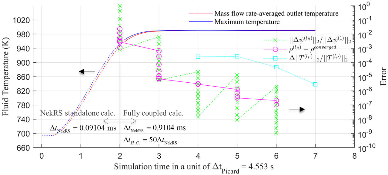
Figure 5: Convergence history of the whole simulation ( - Richardson iteration index, - Picard iteration index.)
Scheme (A) in Figure 2 resulted in false temperature convergence unless the Richardson tolerance was very carefully controlled. This false convergence arises due to the weak coupling nature of temperature and angular flux in this problem, where monitoring the angular flux convergence is not a good proxy for temperature convergence. Figure 6 shows that the power distribution is almost converged with less than 1% error in only one Picard iteration, despite the temperature not being converged. Although not shown, errors in power distribution kept decreasing after the first Picard iteration. This confirms that neutronics is weakly coupled to temperature in this problem, and that neutronics power distributions from early in the simulation will result in an accurate temperature profile.
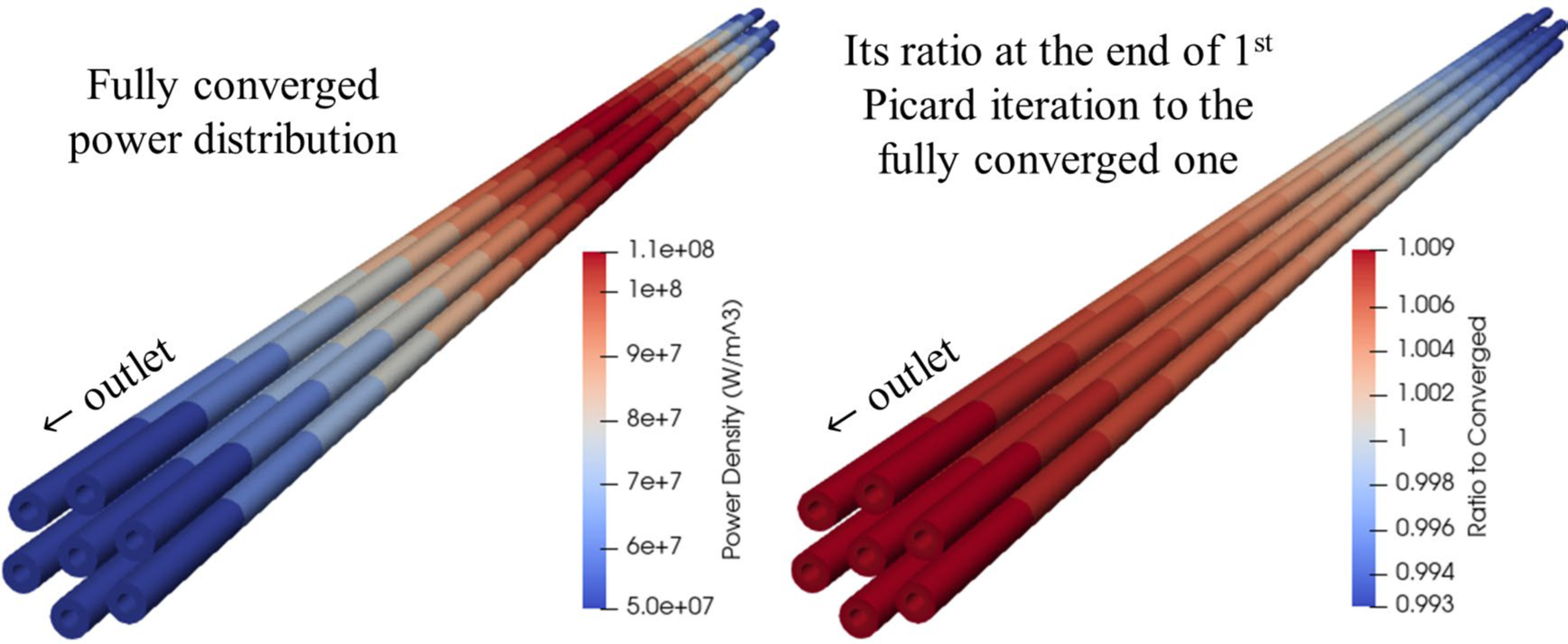
Figure 6: Fast convergence of power distribution due to weak coupling.
One noteworthy observation was that infrequent data communication between H.T. and NekRS may result in solution oscillations. Figure 7 shows that when H.T. is called 10 times less frequently (500:1 rather than 50:1 NekRS:H.T.), a large unphysical fluctuation appears in the solution. Although only the duct heat flux is shown, other solutions also deviate from expected results. This observation is consistent with the fact that the operator splitting method is first order accurate in time, and such an observation would occur with other codes selected for the fluid solve and the solid solve (i.e this effect is not specific to Cardinal or MOOSE).
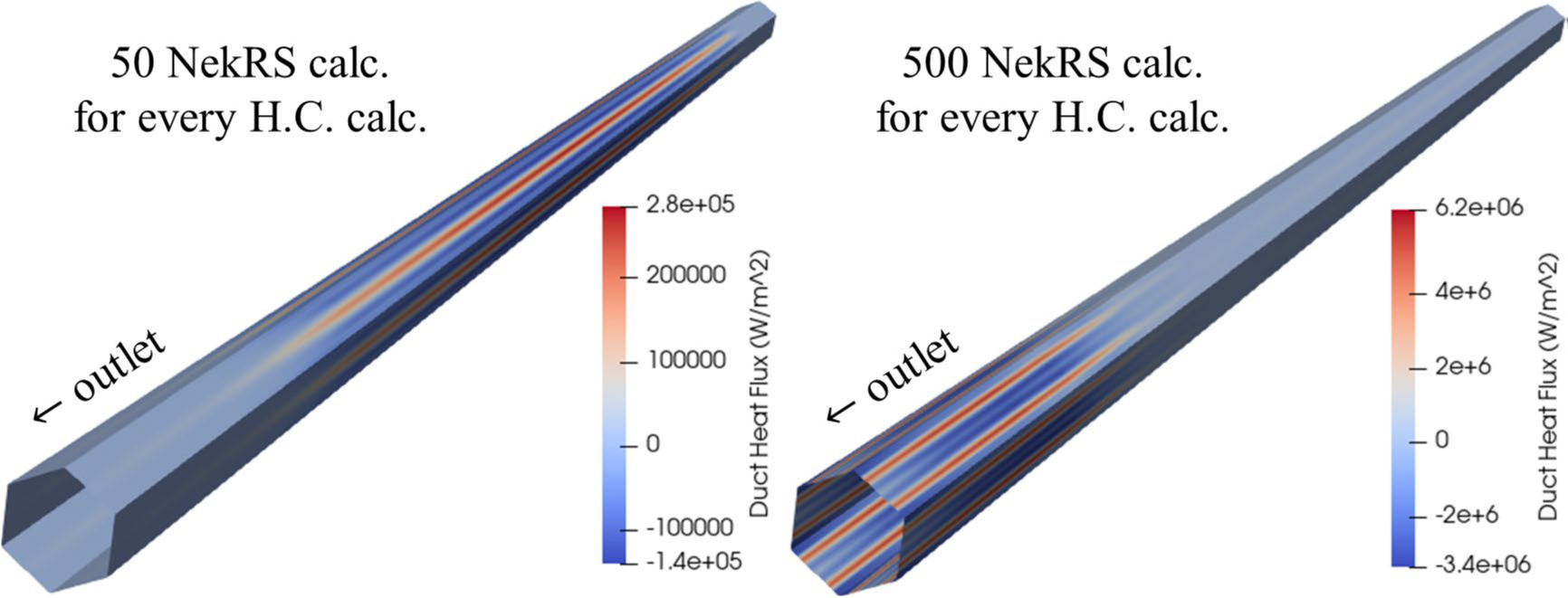
Figure 7: Unphysical pattern of solution (duct heat flux) caused by the infrequent data communication in the conjugate heat transfer with the operator splitting method.
Verification of radial temperature profile and axial speed
The radial temperature profile was verified against an independent STAR-CCM+ calculation. The 7-pin example has a smaller rod-duct gap rod-rod gap. This leads to very low axial speed in the corners of the duct as opposed to the space between the interior fuel rods, as shown in Figure 8a. The slow coolant velocity results in hotter temperature near the corner as opposed to the bundle center (an atypical temperature distribution for fast reactor bundles). An independent STARCCM+ calculation shown in Figure 8b confirmed the atypical temperature profile seen in Figure 8c. As an experiment, forcing a radially uniform axial speed resulted in the more conventionally expected temperature distribution with hotter inner zone coolant as seen in Figure 8d.
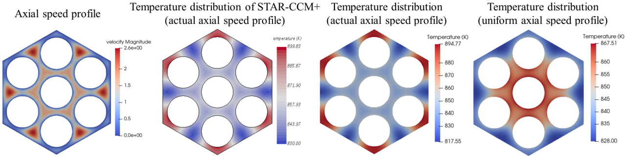
Figure 8: Effect of the axial speed on radial temperature distribution.
Summary and Future works
A multiphysics coupled code system with Griffin, MOOSE heat transfer, and NekRS (Cardinal), has been established using the MOOSE framework for the purpose of hot channel factor evaluation in LFR applications. Griffin drives the coupled simulation using the multiphysics coupling scheme of the DFEM-/CMFD solver. The Richardson iterations for the DFEM-CMFD calculation are performed first, followed by the H.T. and NekRS coupled calculation that uses the operator splitting method for the conjugate heat coupling, in the Picard iteration loop until the relative difference of the L2-norm of the coolant temperature field in successive Picard iterations drops down below . Locating the Picard iteration loop outside the Richardson iteration loop needs to be set in an input manually and is important to avoid false temperature convergence in weakly coupled problems. Special care was taken to align the meshes of different physics solvers and use the most appropriate MOOSE Transfer to increase the accuracy of the data transfer.
The system has been verified for the simplified problem consisting of seven pins with a duct. Global energy conservation was confirmed. The integral of heat fluxes on each solid-fluid interface matched the total power produced inside each solid volume, and the distribution was qualitatively correct. Lessons learned are the need for more frequent data communication when the operator splitting method is used, and the need to carefully check data interpolation between different meshes of different code systems.
Future works include the following.
The 7-pin model will be extended to a whole assembly model.
The MOOSE Stochastic Tools Module (STM) (Slaughter et al., 2023) will be employed to streamline HCF evaluation by sampling input parameters to be perturbed. To this objective, an effort is on-going to perturb native NekRS inputs from STM, use a MOOSE mesh generator to build NekRS mirror and native meshes, and enable multiple runs of NekRS in a single execution of the stochastic tool.
Run Command
Execution of simulations for this Cardinal model may require HPC resources. Specifically, the simulations were conducted on the Idaho National Laboratory HPC cluster, Sawtooth, employing 144 processes. Details of the run script and the associated submission script are presented below.
#!/bin/bash
#PBS -N <your_jobname>
#PBS -l select=4:ncpus=48:mpiprocs=48:mem=190GB:ompthreads=1
#PBS -l walltime=03:00:00
#PBS -m ae
#PBS -j oe
#PBS -P <your_hpc_project>

module load use.moose
module load moose-tools
module load openmpi/4.1.5_ucx1.14.1
module load cmake

export CC=mpicc
export CXX=mpicxx
export FC=mpif90

export WORKING_DIR=<your working directory, ideally on /scratch/ for optimized write latency>
export CARDINAL_DIR=$WORKING_DIR/cardinal
export GRIFFIN_DIR=$WORKING_DIR/griffin
export NEKRS_HOME=$CARDINAL_DIR/install
export ENABLE_OPENMC=false
export NEKRS_OCCA_MODE_DEFAULT=CPU
export MOOSE_DIR=$CARDINAL_DIR/contrib/moose

echo ------------------------------------------------------
echo -n 'Job is running on node\n'; cat $PBS_NODEFILE
echo ------------------------------------------------------
echo PBS: qsub is running on $PBS_O_HOST
echo PBS: executing queue is $PBS_QUEUE
echo PBS: working directory is $PBS_O_WORKDIR
echo PBS: job identifier is $PBS_JOBID
echo PBS: job name is $PBS_JOBNAME
echo PBS: node file is $PBS_NODEFILE
echo PBS: current home directory is $PBS_O_HOME
echo PBS: PATH = $PBS_O_PATH
echo ------------------------------------------------------

#NNODES=`cat $PBS_NODEFILE | wc -l`
#NCPUS=4
#NSLOTS=$((NNODES * NCPUS))

cd $PBS_O_WORKDIR

mpirun $CARDINAL_DIR/cardinal-opt -i NT.i > logfile_144procs
qsub runjob_sawtooth.sh
References
- Paul Fischer, Stefan Kerkemeier, Misun Min, Yu-Hsiang Lan, Malachi Phillips, Thilina Rathnayake, Elia Merzari, Ananias Tomboulides, Ali Karakus, Noel Chalmers, and Tim Warburton.
NekRS, a GPU-accelerated spectral element Navier–Stokes solver.
Parallel Computing, 114:102982, 2022.[BibTeX]
- G Grasso, A Levinsky, F Franceschini, and P Ferroni.
A MOX-fuel core configuration for the Westinghouse Lead Fast Reactor.
In Proceedings of International Congress on Advances in Nuclear Power Plants. France, 2019.[BibTeX]
- Changho Lee, Yeon Sang Jung, Hansol Park, Emily R Shemon, Javier Ortensi, Yaqi Wang, Vincent M Laboure, and Zachary M Prince.
Griffin Software Development Plan.
Technical Report ANL/NSE-21/23, Argonne National Laboratory, Lemont, IL, 2021.
doi:10.2172/1845956.[BibTeX]
- Alexander D Lindsay, Derek R Gaston, Cody J Permann, Jason M Miller, David Andrš, Andrew E Slaughter, Fande Kong, Joshua Hansel, Robert W Carlsen, Casey Icenhour, Logan Harbour, Guillaume L Giudicelli, Roy H Stogner, Peter German, Jacob Badger, Sudipta Biswas, Leora Chapuis, Christopher Green, Jason Hales, Tianchen Hu, Wen Jiang, Yeon Sang Jung, Christopher Matthews, Yinbin Miao, April Novak, John W Peterson, Zachary M Prince, Andrea Rovinelli, Sebastian Schunert, Daniel Schwen, Benjamin W Spencer, Swetha Veeraraghavan, Antonio Recuero, Dewen Yushu, Yaqi Wang, Andy Wilkins, and Christopher Wong.
2.0 - MOOSE: Enabling massively parallel multiphysics simulation.
SoftwareX, 20:101202, 2022.
URL: https://www.sciencedirect.com/science/article/pii/S2352711022001200, doi:10.1016/j.softx.2022.101202.[BibTeX]
- April J. Novak, D Andrs, P Shriwise, Jun Fang, Haomin Yuan, Dillon Shaver, Elia Merzari, Paul K Romano, and R C Martineau.
Coupled Monte Carlo and thermal-fluid modeling of high temperature gas reactors using Cardinal.
Annals of Nuclear Energy, 177:109310, 2022.
doi:10.1016/j.anucene.2022.109310.[BibTeX]
- E R Shemon, Y Yu, and T K Kim.
Applications of SHARP Toolkit to SFR Challenging Problems: Evaluation of Hot Channel Factors and Demonstration of Zooming Capability.
Technical Report ANL/NSE-18/4, Argonne National Laboratory, Lemont, IL, 2018.
doi:10.217Permann20202/1483839.[BibTeX]
- Emily Shemon, Yinbin Miao, Shikhar Kumar, Kun Mo, Yeon Sang Jung, Aaron Oaks, Guillaume Giudicelli, Logan Harbour, and Roy Stogner.
MOOSE Reactor Module Meshing Enhancements to Support Reactor Analysis.
Technical Report ANL/NSE-22/65, Argonne National Laboratory and Idaho National Laboratory, 2022.[BibTeX]
- Emily Shemon, Yiqi Yu, Hansol Park, and Colin Brennan.
Assessment of Fast Reactor Hot Channel Factor Calculation Capability in Griffin and NekRS.
Technical Report ANL/NSE-21/42, Argonne National Laboratory, Lemont, IL, 2021.[BibTeX]
- Andrew E Slaughter, Zachary M Prince, Peter German, Ian Halvic, Wen Jiang, Benjamin W Spencer, Somayajulu L N Dhulipala, and Derek R Gaston.
MOOSE Stochastic Tools: A module for performing parallel, memory-efficient in situ stochastic simulations.
SoftwareX, 22:101345, 2023.
doi:10.1016/j.softx.2023.101345.[BibTeX]
- Yaqi Wang, Changho Lee, Yeon Sang Jung, Zachary Prince, Joshua Hanophy, Logan Harbour, Hansol Park, and Javier Ortensi.
Performance improvements to the griffin transport solvers.
Technical Report INL/EXT-21-64272, Idaho National Laboratory, 2021.[BibTeX]