ver-1fc

Conduction in composite structure with constant surface temperatures

General Case Description

This third heat transfer problem is taken from Ambrosek and Longhurst (2008) and builds on the capabilities verified in ver-1fa and ver-1fb. The configuration is the same as in ver-1fb, except that, the current case is in a composite structure with constant surface temperature. This case is simulated in (test/tests/ver-1fc/ver-1fc.i) with both transient and steady state solutions.

The composite is a 40 cm thick layer of Copper (Cu) followed by a 40 cm layer of iron (Fe) ((Ambrosek and Longhurst, 2008)). The temperature of both layers is initially 0 K, but at time t = 0, the outside face of the Cu is held at 600 K while the outside face of the Fe is maintained at 0 K. The thermal conductivities of Cu and Fe are set to 401 W/m/K and 80.2 W/m/K, respectively. The TMAP7 documentation does not specify the materials' density $var element = document.getElementById("moose-equation-10578f10-c47f-4462-b40d-c733b1522746");katex.render("\\rho", element, {displayMode:false,throwOnError:false});$ or the specific heat $var element = document.getElementById("moose-equation-90fb9f23-f559-4ee9-8f36-7a111fa4b168");katex.render("C_p", element, {displayMode:false,throwOnError:false});$ , but the TMAP7 input file lists $var element = document.getElementById("moose-equation-ae7ce4d8-72ac-4a81-a660-4c6433243332");katex.render("\\rho C_p = 3.4392 \\times 10^6", element, {displayMode:false,throwOnError:false});$ J $var element = document.getElementById("moose-equation-a4994843-77d8-42b2-99c8-00b891505d8e");katex.render("\\cdot", element, {displayMode:false,throwOnError:false});$ m $var element = document.getElementById("moose-equation-b188df70-4590-4105-8b38-990fe586860e");katex.render("^{-3}\\cdot", element, {displayMode:false,throwOnError:false});$ K $var element = document.getElementById("moose-equation-a4583fe1-c2c4-423c-801a-89fe1c807040");katex.render("^{-1}", element, {displayMode:false,throwOnError:false});$ for Cu and $var element = document.getElementById("moose-equation-f240ca0f-d03f-4b57-8b6d-90cafa7e264a");katex.render("3.5179 \\times 10^6", element, {displayMode:false,throwOnError:false});$ J $var element = document.getElementById("moose-equation-e512c319-60c7-4974-a5aa-66208dd89dd2");katex.render("\\cdot", element, {displayMode:false,throwOnError:false});$ m $var element = document.getElementById("moose-equation-3d3c68e0-3365-43e2-92b9-57576735175e");katex.render("^{-3}\\cdot", element, {displayMode:false,throwOnError:false});$ K $var element = document.getElementById("moose-equation-2739c3fe-a2e3-499b-9935-762ef25faac4");katex.render("^{-1}", element, {displayMode:false,throwOnError:false});$ for Fe (Ambrosek and Longhurst, 2008). TMAP8 uses $var element = document.getElementById("moose-equation-e8dc7ed3-ff93-4c54-a9fc-e3cc6de90018");katex.render("\\rho = 8960", element, {displayMode:false,throwOnError:false});$ kg/m $var element = document.getElementById("moose-equation-92c56f85-77f1-422f-b08a-e5e88bae0272");katex.render("^{3}", element, {displayMode:false,throwOnError:false});$ and $var element = document.getElementById("moose-equation-1a957aa1-04e1-44bd-8823-a2bd2a731b12");katex.render("C_p = 383.8", element, {displayMode:false,throwOnError:false});$ J $var element = document.getElementById("moose-equation-cb7198e3-6a24-4fe0-9ff3-0460240e1948");katex.render("\\cdot", element, {displayMode:false,throwOnError:false});$ kg $var element = document.getElementById("moose-equation-ab8ac5e6-656e-45aa-9705-434fff372962");katex.render("^{-1}\\cdot", element, {displayMode:false,throwOnError:false});$ K $var element = document.getElementById("moose-equation-d29ac1fc-a2ae-477b-90d5-ba47a0d66d02");katex.render("^{-1}", element, {displayMode:false,throwOnError:false});$ for Cu and $var element = document.getElementById("moose-equation-07eb0b00-427b-4646-a5ab-71d1429c2c41");katex.render("\\rho = 7870", element, {displayMode:false,throwOnError:false});$ kg/m $var element = document.getElementById("moose-equation-96c70a3c-5a5a-42e7-824d-40acb6fb9b3a");katex.render("^{3}", element, {displayMode:false,throwOnError:false});$ and $var element = document.getElementById("moose-equation-06ae1b6c-4060-462a-8778-f389d9d38689");katex.render("C_p = 447.0", element, {displayMode:false,throwOnError:false});$ J $var element = document.getElementById("moose-equation-a5a3c053-b91a-488b-9602-2b6d79a3cdec");katex.render("\\cdot", element, {displayMode:false,throwOnError:false});$ kg $var element = document.getElementById("moose-equation-999968da-f62d-4e09-abb9-c05efafc98a4");katex.render("^{-1}\\cdot", element, {displayMode:false,throwOnError:false});$ K $var element = document.getElementById("moose-equation-384ee0a7-5d40-491b-883b-a3a2c4673a5f");katex.render("^{-1}", element, {displayMode:false,throwOnError:false});$ for Fe. The densities are from Haynes (2015), and the specific heat capacities are calculated to match the $var element = document.getElementById("moose-equation-5a519f76-772f-44ed-93dd-8300e489bcf5");katex.render("\\rho C_p", element, {displayMode:false,throwOnError:false});$ values from TMAP7 in Ambrosek and Longhurst (2008), which closely match values from Haynes (2015) ( $var element = document.getElementById("moose-equation-64047adf-8439-4de4-80ee-8f6a301936c2");katex.render("C_p = 385", element, {displayMode:false,throwOnError:false});$ J $var element = document.getElementById("moose-equation-c11369b7-d226-41ae-8482-4b49dbeebadc");katex.render("\\cdot", element, {displayMode:false,throwOnError:false});$ kg $var element = document.getElementById("moose-equation-a3dea810-35f2-4a33-ae29-4e62f2e38c01");katex.render("^{-1}\\cdot", element, {displayMode:false,throwOnError:false});$ K $var element = document.getElementById("moose-equation-8eef84f9-56bf-4046-9d1f-21c96247116f");katex.render("^{-1}", element, {displayMode:false,throwOnError:false});$ for Cu and $var element = document.getElementById("moose-equation-023f00a9-7cc8-4468-821d-b5912e1c181e");katex.render("C_p = 449", element, {displayMode:false,throwOnError:false});$ J $var element = document.getElementById("moose-equation-13ab2db8-0a29-45c2-b521-80e5c9bf55d7");katex.render("\\cdot", element, {displayMode:false,throwOnError:false});$ kg $var element = document.getElementById("moose-equation-6cedab09-430b-4929-bbdc-78e66eae93e0");katex.render("^{-1}\\cdot", element, {displayMode:false,throwOnError:false});$ K $var element = document.getElementById("moose-equation-d0042609-8966-4a90-9a4c-ea4897487e92");katex.render("^{-1}", element, {displayMode:false,throwOnError:false});$ for Fe).

This case provides both a verification (comparison against an analytical solution) and a benchmarking (code-to-code comparison) exercise. The steady state solution (called ver-1fcs in Ambrosek and Longhurst (2008)) is compared against an analytical solution, and the transient solution is compared against ABAQUS. ABAQUS is a finite element analysis (FEA) program that has been validated for both transient and steady state solutions in heat transfer modeling applications. The ABAQUS code was setup and run by R. G. Ambrosek and presented in Ambrosek and Longhurst (2008).

warning:Typo in Ambrosek and Longhurst (2008) - confusion between ABAQUS and TMAP7 results

In Ambrosek and Longhurst (2008), Table 11 for TMAP7 and ABAQUS transient results and Table 13 for TMAP7 and ABAQUS steady-state results are identical, even though they should be different. Given the nature of the data, it corresponds to transient conditions and has been used as such for comparison below. As a result, no ABAQUS and TMAP7 data was used in the steady state case, only TMAP8 predictions and the analytical solution. Another issue is that the column labels for ABAQUS and TMAP7 are reversed in Table 11 and Table 13, casting doubt on which results correspond to ABAQUS and which to TMAP7. In this benchmarking exercise, we therefore refer to these results as ABAQUS or TMAP7 (1) and ABAQUS or TMAP7 (2). Since they are close, we still consider the benchmarking exercise successful.

Steady State solution and results

The steady-state solution for this problem was compared to the analytical solution in addition to the ABAQUS prediction from Ambrosek and Longhurst (2008). To solve for the steady state solution for this problem, the heat flux is given by

$(1)var element = document.getElementById("moose-equation-0e161022-5497-4292-b02d-d37917fce7f0");katex.render(" q''=\\frac{T_{SA} - T_{SB}}{\\left(L_A / k_A \\right) + \\left(L_B / k_B \\right)},", element, {displayMode:true,throwOnError:false});$ where

$var element = document.getElementById("moose-equation-f50881b7-1d42-46f9-a0af-2ef5898f7814");katex.render("T_{Si}", element, {displayMode:false,throwOnError:false});$ is the temperature of surface $var element = document.getElementById("moose-equation-9327781b-1435-4880-b717-fa5c39173581");katex.render("i", element, {displayMode:false,throwOnError:false});$ , left ( $var element = document.getElementById("moose-equation-3343dbdd-ab67-4395-ae0d-cf6bcec1f52c");katex.render("T_{SA}=600", element, {displayMode:false,throwOnError:false});$ K) and right ( $var element = document.getElementById("moose-equation-72bb51e2-992b-4a08-bd15-ddf337e63a2e");katex.render("T_{SB}=0", element, {displayMode:false,throwOnError:false});$ K),
$var element = document.getElementById("moose-equation-42877591-d82b-4b9a-8621-3da8b202655b");katex.render("L_i", element, {displayMode:false,throwOnError:false});$ is Length of segment $var element = document.getElementById("moose-equation-11cdeecb-5761-44bf-9dec-8adbc38a2dba");katex.render("i", element, {displayMode:false,throwOnError:false});$ ( $var element = document.getElementById("moose-equation-98ee6570-873a-4a8b-a455-5a6d90105d28");katex.render("L_A=L_B=40", element, {displayMode:false,throwOnError:false});$ cm),
$var element = document.getElementById("moose-equation-7fbaba20-797b-46ef-9ff4-a96c66f0e9af");katex.render("k_i", element, {displayMode:false,throwOnError:false});$ is thermal conductivity of segment $var element = document.getElementById("moose-equation-1080c83c-daeb-41f3-8f28-6b70e6bf45e1");katex.render("i", element, {displayMode:false,throwOnError:false});$ ( $var element = document.getElementById("moose-equation-ccec321e-e843-4769-9eb3-6a48479852c8");katex.render("k_A = 401", element, {displayMode:false,throwOnError:false});$ W/m/K, $var element = document.getElementById("moose-equation-5553749f-73aa-4b3d-833c-193261dbe421");katex.render("k_B = 80.2", element, {displayMode:false,throwOnError:false});$ W/m/K).

At steady state, the flux in and out of any section of the slab are equal. The temperature at the interface ( $var element = document.getElementById("moose-equation-9699f62c-1958-4956-864d-d83cd53176ba");katex.render("T_I", element, {displayMode:false,throwOnError:false});$ ) can be found by setting the flux through A equal to the flux through B, which leads to:

$(2)var element = document.getElementById("moose-equation-8c4668b9-512b-420a-b9c9-a27d9d7d2f8d");katex.render(" \\frac{T_{SA} - T_{I}}{\\left(L_A / k_A \\right)} = \\frac{T_{I} - T_{SB}}{\\left(L_B / k_B \\right)}.", element, {displayMode:true,throwOnError:false});$

The interface temperature at steady state is therefore equal to $var element = document.getElementById("moose-equation-29cd4210-a432-46f3-b070-0e682e91a6ff");katex.render("T_I = 500", element, {displayMode:false,throwOnError:false});$ K. The temperature profile for conduction in steady state, with constant physical properties, is linear. The temperature profile of A and B can therefore be found through linear interpolation.

With TMAP8, the steady state solution can be obtained in different ways: by using the steady state solve or by running a transient simulation until steady state is reached. Ambrosek and Longhurst (2008) indicates that the steady state solution was obtained by running the transient solution until $var element = document.getElementById("moose-equation-0328a93d-887b-46e6-a560-290d3f1253f1");katex.render("t=10,000", element, {displayMode:false,throwOnError:false});$ s, which is what is reproduced with TMAP8 here. TMAP8 predictions were found to be identical to the analytical solution with a root mean square percentage error (RMSPE) of 0.23 %, as shown in Figure 1.

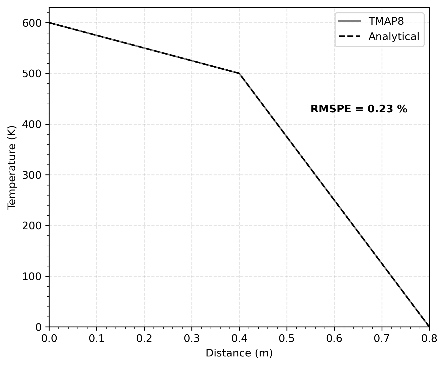
Figure 1: Comparison of temperature profiles from the analytical solution and TMAP8 in the composite structure at steady state ( $var element = document.getElementById("moose-equation-5bfe1b12-5000-4b84-a0c5-16695422a22a");katex.render("t = 10000", element, {displayMode:false,throwOnError:false});$ s). RMSPE is the root mean square percentage error between the analytical and TMAP8 profiles.

Transient solution and results

For the transient case, TMAP8 predictions are compared against ABAQUS predictions from Ambrosek and Longhurst (2008). This is therefore a benchmarking case.

The transient solution was compared in two ways: where time, $var element = document.getElementById("moose-equation-70db47af-3575-4493-870a-07cc06f4e292");katex.render("t", element, {displayMode:false,throwOnError:false});$ , is held constant and where distance, $var element = document.getElementById("moose-equation-988b0c94-3afb-4595-8529-78ffca263bf7");katex.render("x", element, {displayMode:false,throwOnError:false});$ , through the structure is held constant. The constant time comparison between ABAQUS and TMAP8 was made at time $var element = document.getElementById("moose-equation-4b1ef070-805b-4b91-968f-a2426d4e1af6");katex.render("t = 150", element, {displayMode:false,throwOnError:false});$ s. The constant time values are shown in Figure 2, and the comparison is satisfactory.

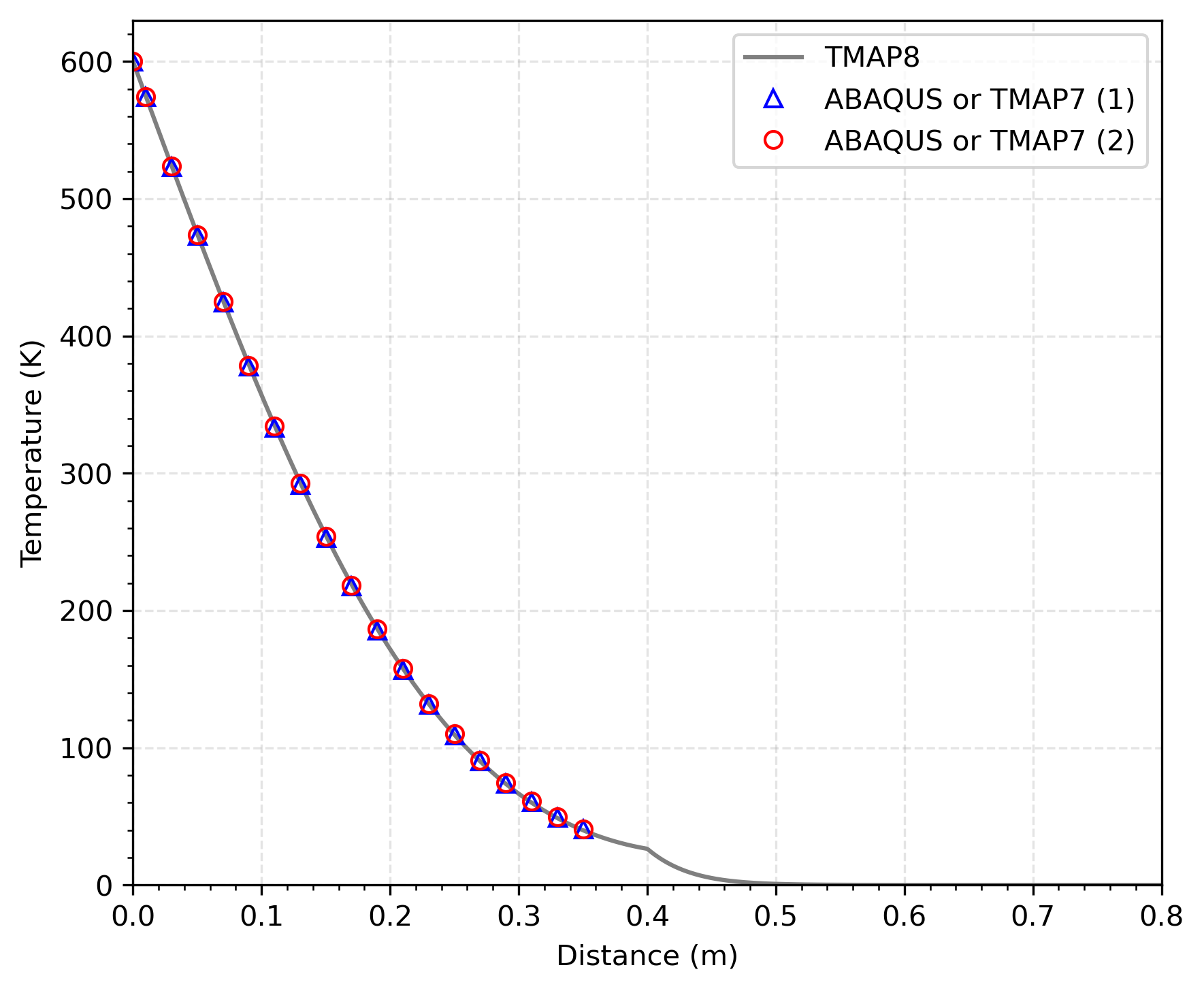
Figure 2: Comparison of temperature profiles from TMAP8, TMAP7, and ABAQUS in the composite structure at $var element = document.getElementById("moose-equation-51efbf2c-daaa-4d64-b516-50105768c8fb");katex.render("t = 150", element, {displayMode:false,throwOnError:false});$ s.

The constant distance values were compared at $var element = document.getElementById("moose-equation-d8efbaab-9ece-4991-99b9-c3a571674dff");katex.render("x = 0.09", element, {displayMode:false,throwOnError:false});$ m, at 5 second intervals from time $var element = document.getElementById("moose-equation-e4c00916-e8da-47f0-b636-0e0cd4105a6f");katex.render("t = 0", element, {displayMode:false,throwOnError:false});$ s to $var element = document.getElementById("moose-equation-fdca8525-2f90-4af1-8de1-47329d88bae9");katex.render("t = 150", element, {displayMode:false,throwOnError:false});$ s. These results can be seen in Figure 3, and the comparison is satisfactory.

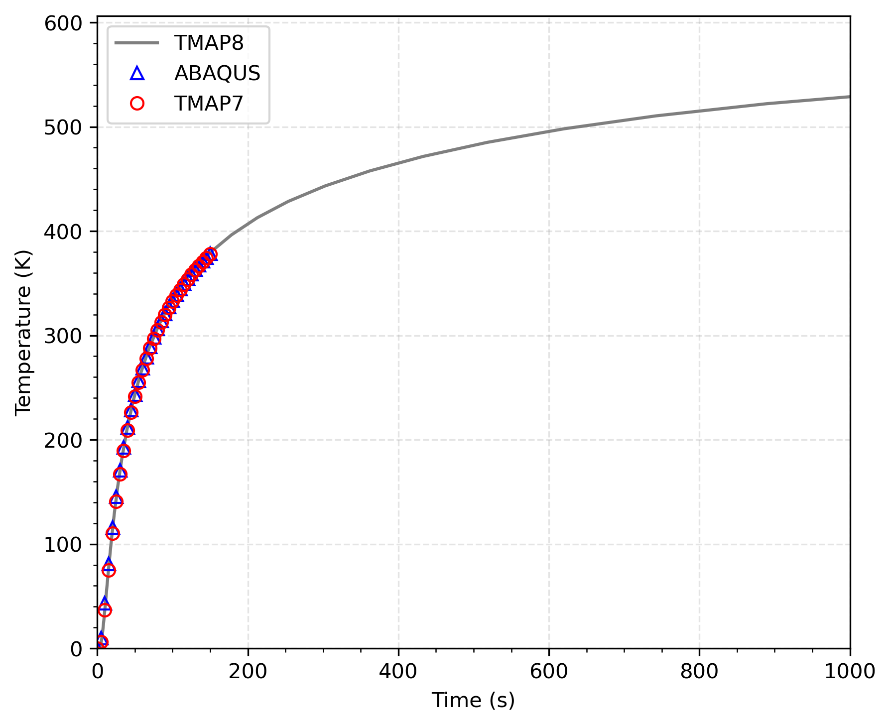
Figure 3: Comparison of temperature value over time from TMAP8, TMAP7, and ABAQUS in the composite structure at $var element = document.getElementById("moose-equation-24458b1e-3c7a-43f3-968e-26eff92a0504");katex.render("x = 0.09", element, {displayMode:false,throwOnError:false});$ m.

Input files

The input file for this case can be found at (test/tests/ver-1fc/ver-1fc.i), which is also used as test in TMAP8 at (test/tests/ver-1fc/tests).

References

James Ambrosek and GR Longhurst. Verification and Validation of TMAP7. Technical Report INEEL/EXT-04-01657, Idaho National Engineering and Environmental Laboratory, December 2008.

@techreport{ambrosek2008verification,
    author = "Ambrosek, James and Longhurst, GR",
    title = "{Verification and Validation of TMAP7}",
    year = "2008",
    number = "INEEL/EXT-04-01657",
    month = "December",
    institution = "Idaho National Engineering and Environmental Laboratory"
}

W. M. Haynes. CRC Handbook of Chemistry and Physics. CRC Press/Taylor and Francis, 95th edition, 2015.

@book{Haynes2015,
    author = "Haynes, W. M.",
    editor = "Haynes, W. M. and Lide, David R. and Bruno, Thomas J.",
    city = "Boca Raton, FL",
    edition = "95th",
    publisher = "CRC Press/Taylor and Francis",
    title = "{CRC} Handbook of Chemistry and Physics",
    year = "2015"
}

(test/tests/ver-1fc/ver-1fc.i)

# Verification Problem #1fc from TMAP7 V&V document
# Thermal conduction in composite structure with constant surface temperatures

# Data used in TMAP7 case
T_SA = '${units 600 K}'
T_SB = '${units 0 K}'
L_A = '${units 0.4 m}'
L_B = '${units 0.4 m}'
k_A = '${units 401 W/m/K}'
k_B = '${units 80.2 W/m/K}'
position_measurement = '${units 9e-2 m}'
density_Cu = '${units 8960 kg/m^3}'
specific_heat_Cu = '${units 383.8 J/kg/K}'
density_Fe = '${units 7870 kg/m^3}'
specific_heat_Fe = '${units 447.0 J/kg/K}'

# Data selected for TMAP8 case
num_nodes = 800 # (-)

[Mesh]
  [whole_domain]
    type = GeneratedMeshGenerator
    xmin = 0
    xmax = '${fparse L_A + L_B}'
    dim = 1
    nx = ${num_nodes}
  []
  [injection_block_1]
    type = ParsedSubdomainMeshGenerator
    input = whole_domain
    combinatorial_geometry = 'x < ${L_A}'
    block_id = 0
  []
  [injection_block_2]
    type = ParsedSubdomainMeshGenerator
    input = injection_block_1
    combinatorial_geometry = 'x > ${L_A}'
    block_id = 1
  []
[]

[Variables]
  # temperature parameter in the slab in K
  [temperature]
    initial_condition = 0.0
    scaling = 1e-6
  []
[]

[Functions]
  [thermal_conductivity_func_Cu]
    type = ParsedFunction
    expression = ${k_A}
  []
  [thermal_conductivity_func_Fe]
    type = ParsedFunction
    expression = ${k_B}
  []
[]

[Kernels]
  [heat]
    type = HeatConduction
    variable = temperature
  []
  [HeatTdot]
    type = HeatConductionTimeDerivative
    variable = temperature
  []
[]

[BCs]
  # The temperature on the left boundary of the slab is kept constant
  [lefttemperature]
    type = DirichletBC
    boundary = left
    variable = temperature
    value = ${T_SA}
  []
  # The temperature on the right boundary of the slab is kept constant
  [righttemperature]
    type = DirichletBC
    boundary = right
    variable = temperature
    value = ${T_SB}
  []
[]

[Materials]
  # the specific heat of Cu layer
  [specific_heat_Cu]
    type = GenericConstantMaterial
    block = '0'
    prop_names = 'density specific_heat'
    prop_values = '${density_Cu} ${specific_heat_Cu}'
  []
  # the specific heat of Fe layer
  [specific_heat_Fe]
    type = GenericConstantMaterial
    block = '1'
    prop_names = 'density specific_heat'
    prop_values = '${density_Fe} ${specific_heat_Fe}'
  []
  # the thermal conductivity of Cu layer
  [thermal_conductivity_Cu]
    type = GenericFunctionMaterial
    block = '0'
    prop_values = thermal_conductivity_func_Cu
    prop_names = thermal_conductivity
    outputs = exodus
  []
  # the thermal conductivity of Fe layer
  [thermal_conductivity_Fe]
    type = GenericFunctionMaterial
    block = '1'
    prop_values = thermal_conductivity_func_Fe
    prop_names = thermal_conductivity
    outputs = exodus
  []
[]

[Preconditioning]
  [SMP]
    type = SMP
    full = true
  []
[]

[Executioner]
  type = Transient
  scheme = bdf2
  solve_type = NEWTON
  petsc_options_iname = '-pc_type'
  petsc_options_value = 'lu'
  nl_rel_tol = 1e-50
  nl_abs_tol = 1e-12
  l_tol = 1e-8
  dtmax = 5e2
  end_time = 10000
  [TimeStepper]
    type = IterationAdaptiveDT
    dt = 1e-1
    optimal_iterations = 3
    iteration_window = 1
    growth_factor = 1.2
    cutback_factor = 0.8
  []
[]

[Postprocessors]
  # Used to obtain varying temperature with time at x=0.09 m
  [temperature_at_x]
    type = PointValue
    variable = temperature
    point = '${position_measurement} 0 0'
    outputs = 'csv'
  []
[]

[VectorPostprocessors]
  # Used to obtain the temperature distribution with time at corresponding time
  [line]
    type = LineValueSampler
    start_point = '0 0 0'
    end_point = '${fparse L_A + L_B} 0 0'
    num_points = ${num_nodes}
    sort_by = 'x'
    variable = temperature
    outputs = vector_postproc
  []
[]

[Outputs]
  exodus = true
  [csv]
    type = CSV
    file_base = 'ver-1fc_temperature_at_x0.09'
  []
  [vector_postproc]
    type = CSV
    sync_times = '150 10000'
    sync_only = true
  []
[]

(test/tests/ver-1fc/ver-1fc.i)

# Verification Problem #1fc from TMAP7 V&V document
# Thermal conduction in composite structure with constant surface temperatures

# Data used in TMAP7 case
T_SA = '${units 600 K}'
T_SB = '${units 0 K}'
L_A = '${units 0.4 m}'
L_B = '${units 0.4 m}'
k_A = '${units 401 W/m/K}'
k_B = '${units 80.2 W/m/K}'
position_measurement = '${units 9e-2 m}'
density_Cu = '${units 8960 kg/m^3}'
specific_heat_Cu = '${units 383.8 J/kg/K}'
density_Fe = '${units 7870 kg/m^3}'
specific_heat_Fe = '${units 447.0 J/kg/K}'

# Data selected for TMAP8 case
num_nodes = 800 # (-)

[Mesh]
  [whole_domain]
    type = GeneratedMeshGenerator
    xmin = 0
    xmax = '${fparse L_A + L_B}'
    dim = 1
    nx = ${num_nodes}
  []
  [injection_block_1]
    type = ParsedSubdomainMeshGenerator
    input = whole_domain
    combinatorial_geometry = 'x < ${L_A}'
    block_id = 0
  []
  [injection_block_2]
    type = ParsedSubdomainMeshGenerator
    input = injection_block_1
    combinatorial_geometry = 'x > ${L_A}'
    block_id = 1
  []
[]

[Variables]
  # temperature parameter in the slab in K
  [temperature]
    initial_condition = 0.0
    scaling = 1e-6
  []
[]

[Functions]
  [thermal_conductivity_func_Cu]
    type = ParsedFunction
    expression = ${k_A}
  []
  [thermal_conductivity_func_Fe]
    type = ParsedFunction
    expression = ${k_B}
  []
[]

[Kernels]
  [heat]
    type = HeatConduction
    variable = temperature
  []
  [HeatTdot]
    type = HeatConductionTimeDerivative
    variable = temperature
  []
[]

[BCs]
  # The temperature on the left boundary of the slab is kept constant
  [lefttemperature]
    type = DirichletBC
    boundary = left
    variable = temperature
    value = ${T_SA}
  []
  # The temperature on the right boundary of the slab is kept constant
  [righttemperature]
    type = DirichletBC
    boundary = right
    variable = temperature
    value = ${T_SB}
  []
[]

[Materials]
  # the specific heat of Cu layer
  [specific_heat_Cu]
    type = GenericConstantMaterial
    block = '0'
    prop_names = 'density specific_heat'
    prop_values = '${density_Cu} ${specific_heat_Cu}'
  []
  # the specific heat of Fe layer
  [specific_heat_Fe]
    type = GenericConstantMaterial
    block = '1'
    prop_names = 'density specific_heat'
    prop_values = '${density_Fe} ${specific_heat_Fe}'
  []
  # the thermal conductivity of Cu layer
  [thermal_conductivity_Cu]
    type = GenericFunctionMaterial
    block = '0'
    prop_values = thermal_conductivity_func_Cu
    prop_names = thermal_conductivity
    outputs = exodus
  []
  # the thermal conductivity of Fe layer
  [thermal_conductivity_Fe]
    type = GenericFunctionMaterial
    block = '1'
    prop_values = thermal_conductivity_func_Fe
    prop_names = thermal_conductivity
    outputs = exodus
  []
[]

[Preconditioning]
  [SMP]
    type = SMP
    full = true
  []
[]

[Executioner]
  type = Transient
  scheme = bdf2
  solve_type = NEWTON
  petsc_options_iname = '-pc_type'
  petsc_options_value = 'lu'
  nl_rel_tol = 1e-50
  nl_abs_tol = 1e-12
  l_tol = 1e-8
  dtmax = 5e2
  end_time = 10000
  [TimeStepper]
    type = IterationAdaptiveDT
    dt = 1e-1
    optimal_iterations = 3
    iteration_window = 1
    growth_factor = 1.2
    cutback_factor = 0.8
  []
[]

[Postprocessors]
  # Used to obtain varying temperature with time at x=0.09 m
  [temperature_at_x]
    type = PointValue
    variable = temperature
    point = '${position_measurement} 0 0'
    outputs = 'csv'
  []
[]

[VectorPostprocessors]
  # Used to obtain the temperature distribution with time at corresponding time
  [line]
    type = LineValueSampler
    start_point = '0 0 0'
    end_point = '${fparse L_A + L_B} 0 0'
    num_points = ${num_nodes}
    sort_by = 'x'
    variable = temperature
    outputs = vector_postproc
  []
[]

[Outputs]
  exodus = true
  [csv]
    type = CSV
    file_base = 'ver-1fc_temperature_at_x0.09'
  []
  [vector_postproc]
    type = CSV
    sync_times = '150 10000'
    sync_only = true
  []
[]

(test/tests/ver-1fc/tests)

[Tests]
  design = 'HeatConduction.md HeatConductionTimeDerivative.md'
  verification = 'ver-1fc.md'
  issues = '#12 #102'
  [ver-1fc]
    type = Exodiff
    input = ver-1fc.i
    exodiff = ver-1fc_out.e
    requirement = 'The system shall be able to model conduction in a composite structure with constant surface temperatures.'
  []
  [ver-1fc_csvdiff_transient]
    type = CSVDiff
    input = ver-1fc.i
    should_execute = False  # this test relies on the output files from ver-1fc, so it shouldn't be run twice
    csvdiff = ver-1fc_temperature_at_x0.09.csv
    requirement = 'The system shall be able to model conduction in a composite structure with constant surface temperatures to generate CSV data for use in comparisons with ABAQUS during transient at x=0.09 m.'
    prereq = ver-1fc
  []
  [ver-1fc_csvdiff_transient_profile]
    type = CSVDiff
    input = ver-1fc.i
    should_execute = False  # this test relies on the output files from ver-1fc, so it shouldn't be run twice
    csvdiff = ver-1fc_vector_postproc_line_0032.csv
    requirement = 'The system shall be able to model conduction in a composite structure with constant surface temperatures to generate CSV data for use in comparisons with ABAQUS during transient at t=150 s.'
    prereq = ver-1fc
  []
  [ver-1fc_csvdiff_steady_state]
    type = CSVDiff
    input = ver-1fc.i
    should_execute = False  # this test relies on the output files from ver-1fc, so it shouldn't be run twice
    csvdiff = ver-1fc_vector_postproc_line_0063.csv
    requirement = 'The system shall be able to model conduction in a composite structure with constant surface temperatures to generate CSV data for use in comparisons with ABAQUS and an analytical solution at steady state (t=10000 s).'
    prereq = ver-1fc
  []
  [ver-1fc_comparison]
    type = RunCommand
    command = 'python3 comparison_ver-1fc.py'
    requirement = 'The system shall be able to generate comparison plots between the analytical solution, ABAQUS data, and simulated solution of verification case 1fc, modeling conduction in a composite structure with constant surface temperatures.'
    required_python_packages = 'matplotlib numpy pandas os'
  []
[]

General Case Description
Steady State solution and results
Transient solution and results
Input files
References