- orderOrder of time integration
C++ Type:MooseEnum
Unit:(no unit assumed)
Controllable:No
Description:Order of time integration
ExplicitSSPRungeKutta
Introduction
This time integrator includes explicit Strong Stability Preserving (SSP) Runge-Kutta time integration methods, of orders 1, 2, and 3, deriving from ExplicitTimeIntegrator, meaning that no nonlinear solver is invoked. The key feature of SSP Runge-Kutta methods is that they preserve the strong stability properties (in any norm or seminorm) of the explicit/forward Euler method Gottlieb (2005).
Formulation
For the ODE the SSP Runge-Kutta methods up to order 3 can be expressed in the following form for a time step: where is the number of stages and for methods up to order 3, is also the order of accuracy. The coefficients , , and can be conveniently expressed in the following tabular form: Respectively, the tables for the methods of orders 1, 2, and 3 are as follows: These methods have the following time step size requirement for stability: where is the maximum time step size for stability of the forward Euler method. For these methods of order 1, 2, 3, .
In MOOSE, generally the system of ODEs to be solved result from discretization using the finite element method, and thus a mass matrix exists: In this case, the stage solution is actually the following: As an implementation note, the usual mass matrix entry is However, in MOOSE, the mass matrix includes the time step size: (1)
Dirichlet Boundary Conditions Treatment
Now consider the case where one or more degrees of freedom are subject to strong (Dirichlet) boundary conditions: For a nonlinear solve with Newton's method, each iteration consists of the solution of a linear system: (2) and then updating the solution: In MOOSE, Dirichlet boundary conditions are implemented by modifying the residual vector to replace entries for the affected degrees of freedom: By modifying the Jacobian matrix as follows, one can guarantee that the boundary conditions are enforced, i.e., for : To work with MOOSE's Dirichlet boundary condition implementation, Eq. (1) must be put in an update form, similar to Eq. (2): (3) (4) To impose the Dirichlet boundary conditions, the mass matrix and right-hand side vector are modified as for the Newton case: (5) where is an appropriate value to impose for degree of freedom in stage . For most cases, this is simply However, in general, certain conditions must be enforced on the imposed boundary values for intermediate stages to preserve the formal order of accuracy of the method. For methods up to order 2, it is safe to impose each stage as shown above. For the 3rd-order method, the boundary values imposed in each stage should be as follows, according to Zhao and Huang (2019):
The convergence rates for a MMS problem with time-dependent Dirichlet boundary conditions is shown in Figure 1. This illustrates the degradation of the 3rd-order method to 1st-order accuracy in the presence of time-dependent Dirichlet boundary conditions. Contrast this to Figure 2, which shows the results for an MMS problem without time-dependent Dirichlet boundary conditions, demonstrating the expected orders of accuracy.
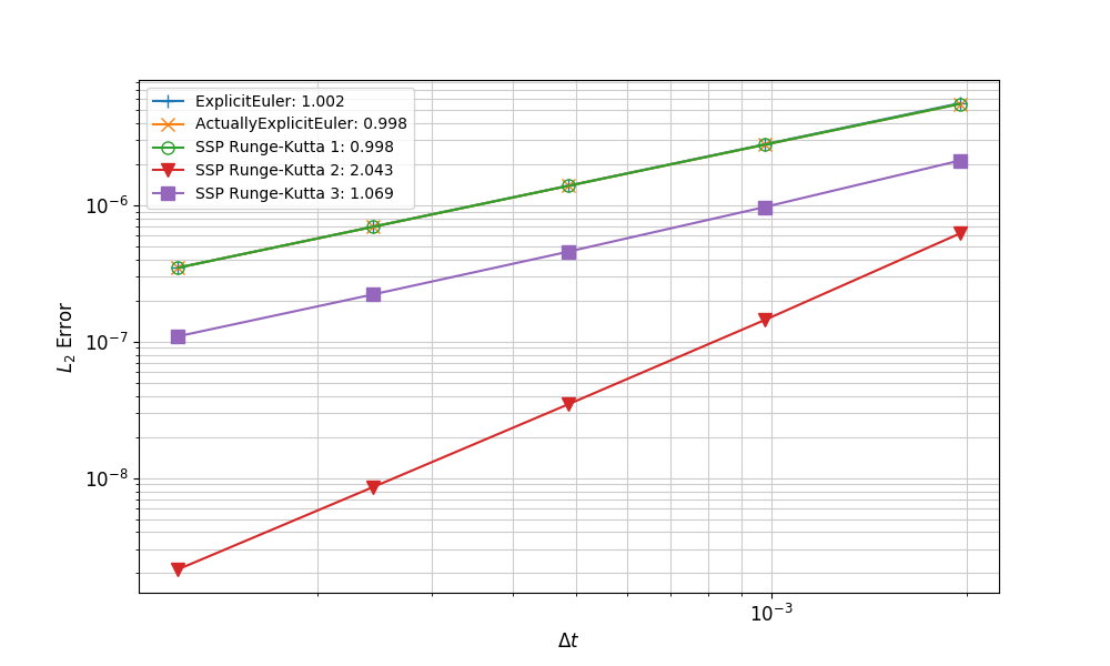
Figure 1: Convergence rates for SSPRK methods on an MMS problem with time-dependent Dirichlet boundary conditions
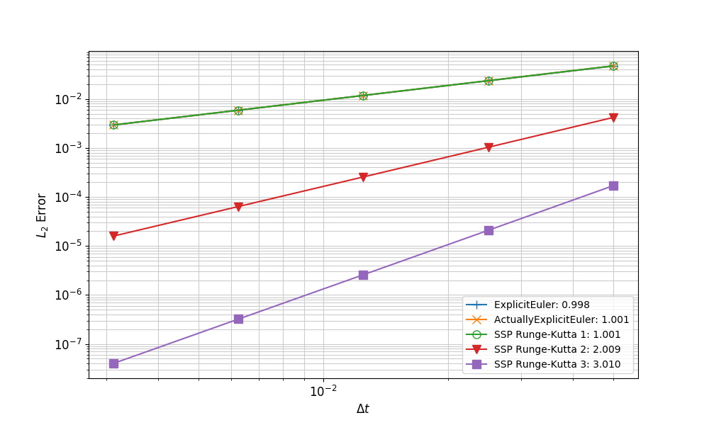
Figure 2: Convergence rates for SSPRK methods on an MMS problem without time-dependent Dirichlet boundary conditions
Implementation
Eq. (3) is implemented as described in the following sections:
computeTimeDerivatives()
Only the Jacobian _du_dot_du is implemented, which is needed by the mass matrix. The time derivative itself is not needed because only part of it appears in the residual vector.
solveStage()
First the mass matrix is computed by calling computeJacobianTag() with the time tag. Because the mass matrix is computed before the call computeResidual(), the call to computeTimeDerivatives() must be made before computeJacobianTag(), even though it will be called again in computeResidual(). The Jacobian must be computed before the call to computeResidual() because the mass matrix will be used in computeResidual() via the call to postResidual(). In computeResidual(), the following steps occur:
postResidual()
Here is assembled as shown in Eq. (4). The mass matrix product here is responsible for the need to call computeJacobianTag() before computeResidual() in solveStage().
Input Parameters
- solve_typeconsistentThe way to solve the system. A 'consistent' solve uses the full mass matrix and actually needs to use a linear solver to solve the problem. 'lumped' uses a lumped mass matrix with a simple inversion - incredibly fast but may be less accurate. 'lump_preconditioned' uses the lumped mass matrix as a preconditioner for the 'consistent' solve
Default:consistent
C++ Type:MooseEnum
Unit:(no unit assumed)
Options:consistent, lumped, lump_preconditioned
Controllable:No
Description:The way to solve the system. A 'consistent' solve uses the full mass matrix and actually needs to use a linear solver to solve the problem. 'lumped' uses a lumped mass matrix with a simple inversion - incredibly fast but may be less accurate. 'lump_preconditioned' uses the lumped mass matrix as a preconditioner for the 'consistent' solve
Optional Parameters
- control_tagsAdds user-defined labels for accessing object parameters via control logic.
C++ Type:std::vector<std::string>
Unit:(no unit assumed)
Controllable:No
Description:Adds user-defined labels for accessing object parameters via control logic.
- enableTrueSet the enabled status of the MooseObject.
Default:True
C++ Type:bool
Unit:(no unit assumed)
Controllable:No
Description:Set the enabled status of the MooseObject.
Advanced Parameters
Input Files
- (modules/navier_stokes/test/tests/finite_volume/cns/benchmark_shock_tube_1D/hllc_sod_shocktube.i)
- (modules/thermal_hydraulics/test/tests/problems/william_louis/3pipes_open.i)
- (modules/thermal_hydraulics/test/tests/problems/lax_shock_tube/lax_shock_tube.i)
- (modules/thermal_hydraulics/test/tests/problems/william_louis/4pipes_closed.i)
- (modules/thermal_hydraulics/test/tests/problems/sod_shock_tube/sod_shock_tube.i)
- (modules/navier_stokes/test/tests/finite_volume/cns/implicit_bcs/hllc_sod_shocktube.i)
- (modules/thermal_hydraulics/test/tests/problems/mms/mms_1phase.i)
- (modules/navier_stokes/test/tests/finite_volume/cns/symmetry_test/2D_symmetry.i)
- (modules/navier_stokes/test/tests/finite_volume/cns/stagnation_inlet/supersonic_nozzle_hllc.i)
- (modules/thermal_hydraulics/test/tests/problems/abrupt_area_change_liquid/base.i)
- (test/tests/time_integrators/explicit_ssp_runge_kutta/explicit_ssp_runge_kutta.i)
- (modules/thermal_hydraulics/test/tests/problems/woodward_colella_blast_wave/woodward_colella_blast_wave.i)
- (modules/navier_stokes/test/tests/finite_volume/cns/shock_tube_2D_cavity/hllc_sod_shocktube_2D.i)
- (modules/thermal_hydraulics/test/tests/problems/sedov_blast_wave/sedov_blast_wave.i)
- (modules/thermal_hydraulics/test/tests/problems/square_wave/square_wave.i)
- (modules/thermal_hydraulics/test/tests/problems/double_rarefaction/1phase.i)
References
- Sigal Gottlieb.
On high order strong stability preserving runge-kutta and multi step time discretizations.
Journal of Scientific Computing, November 2005.
doi:10.1007/s10915-004-4635-5.[BibTeX]
@article{gottlieb2005, author = "Gottlieb, Sigal", title = "On High Order Strong Stability Preserving Runge-Kutta and Multi Step Time Discretizations", journal = "Journal of Scientific Computing", volume = "25", number = "1/2", month = "November", year = "2005", doi = "10.1007/s10915-004-4635-5" } - Weifeng Zhao and Juntao Huang.
Boundary treatment of implicit-explicit Runge-Kutta method for hyperbolic systems with source terms.
arXiv e-prints, pages arXiv:1908.01027, Aug 2019.
arXiv:1908.01027.[BibTeX]
@article{zhao2019,
    author = "{Zhao}, Weifeng and {Huang}, Juntao",
    title = "{Boundary treatment of implicit-explicit Runge-Kutta method for hyperbolic systems with source terms}",
    journal = "arXiv e-prints",
    keywords = "Mathematics - Numerical Analysis",
    year = "2019",
    month = "Aug",
    eid = "arXiv:1908.01027",
    pages = "arXiv:1908.01027",
    archivePrefix = "arXiv",
    eprint = "1908.01027",
    primaryClass = "math.NA",
    adsurl = "https://ui.adsabs.harvard.edu/abs/2019arXiv190801027Z",
    adsnote = "Provided by the SAO/NASA Astrophysics Data System"
}
(modules/navier_stokes/test/tests/finite_volume/cns/benchmark_shock_tube_1D/hllc_sod_shocktube.i)
rho_left = 1
E_left = 2.501505578
u_left = 1e-15

rho_right = 0.125
E_right = 1.999770935
u_right = 1e-15

middle = 50

[GlobalParams]
  fp = fp
[]

[Mesh]
  [cartesian]
    type = GeneratedMeshGenerator
    dim = 1
    xmin = 0
    xmax = ${fparse 2 * middle}
    nx = 1000
  []
[]

[FluidProperties]
  [fp]
    type = IdealGasFluidProperties
  []
[]

[Variables]
  [rho]
    order = CONSTANT
    family = MONOMIAL
    fv = true
  []
  [rho_u]
    order = CONSTANT
    family = MONOMIAL
    fv = true
  []
  [rho_E]
    order = CONSTANT
    family = MONOMIAL
    fv = true
  []
[]

[AuxVariables]
  [rho_a]
    order = CONSTANT
    family = MONOMIAL
  []
[]

[FVKernels]
  [mass_time]
    type = FVTimeKernel
    variable = rho
  []

  [mass_advection]
    type = CNSFVMassHLLC
    variable = rho
  []

  [momentum_time]
    type = FVTimeKernel
    variable = rho_u
  []

  [momentum_advection]
    type = CNSFVMomentumHLLC
    variable = rho_u
    momentum_component = x
  []

  [fluid_energy_time]
    type = FVTimeKernel
    variable = rho_E
  [../]

  [fluid_energy_advection]
    type = CNSFVFluidEnergyHLLC
    variable = rho_E
  []
[]

[FVBCs]
  [mass_implicit]
    type = CNSFVHLLCMassImplicitBC
    variable = rho
    fp = fp
    boundary = 'left right'
  []

  [mom_implicit]
    type = CNSFVHLLCMomentumImplicitBC
    variable = rho_u
    momentum_component = x
    fp = fp
    boundary = 'left right'
  []

  [fluid_energy_implicit]
    type = CNSFVHLLCFluidEnergyImplicitBC
    variable = rho_E
    fp = fp
    boundary = 'left right'
  []
[]

[ICs]
  [rho_ic]
    type = FunctionIC
    variable = rho
    function = 'if (x < ${middle}, ${rho_left}, ${rho_right})'
  []

  [rho_u_ic]
    type = FunctionIC
    variable = rho_u
    function = 'if (x < ${middle}, ${fparse rho_left * u_left}, ${fparse rho_right * u_right})'
  []

  [rho_E_ic]
    type = FunctionIC
    variable = rho_E
    function = 'if (x < ${middle}, ${fparse E_left * rho_left}, ${fparse E_right * rho_right})'
  []
[]

[Materials]
  [var_mat]
    type = ConservedVarValuesMaterial
    rho = rho
    rhou = rho_u
    rho_et = rho_E
    fp = fp
  []
[]

[Preconditioning]
  active = ''
  [./smp]
    type = SMP
    full = true
    petsc_options_iname = '-pc_type'
    petsc_options_value = 'lu'
  [../]
[]

[Executioner]
  type = Transient
  [TimeIntegrator]
    type = ExplicitSSPRungeKutta
    order = 2
  []
  l_tol = 1e-8

  start_time = 0.0
  dt = 1e-2
  end_time = 20
  abort_on_solve_fail = true
[]

[Outputs]
  exodus = true
  perf_graph = true
[]
(modules/thermal_hydraulics/test/tests/problems/william_louis/3pipes_open.i)
# Junction of 3 pipes:
#
#   1     3
# -----*-----
#      | 2
#
# The left end of Pipe 1 is a high-pressure region, and the rest of the system
# is at a low pressure.
#
# Pipe 1 is closed, while Pipes 2 and 3 are open.

end_time = 0.07

D_pipe = 0.01
A_pipe = ${fparse 0.25 * pi * D_pipe^2}
length_pipe1_HP = 0.53
length_pipe1_LP = 3.10
length_pipe2 = 2.595
length_pipe3 = 1.725

x_junction = ${fparse length_pipe1_HP + length_pipe1_LP}

# Numbers of elements correspond to dx ~ 1/3 cm
n_elems_pipe1_HP = 159
n_elems_pipe1_LP = 930
n_elems_pipe2 = 779
n_elems_pipe3 = 518

S_junction = ${fparse 3 * A_pipe}
r_junction = ${fparse sqrt(S_junction / (4 * pi))}
V_junction = ${fparse 4/3 * pi * r_junction^3}

p_low = 1e5
p_high = 1.15e5

T_low  = 283.5690633 # at p = 1e5 Pa,    rho = 1.23 kg/m^3
T_high = 283.5690633 # at p = 1.15e5 Pa, rho = 1.4145 kg/m^3

cfl = 0.95

[GlobalParams]
  # common FlowChannel1Phase parameters
  A = ${A_pipe}
  initial_vel = 0
  fp = fp_air
  closures = closures
  f = 0
  gravity_vector = '0 0 0'
  scaling_factor_1phase = '1 1 1e-5'
[]

[FluidProperties]
  [fp_air]
    type = IdealGasFluidProperties
    gamma = 1.4
    molar_mass = 0.029
  []
[]

[Closures]
  [closures]
    type = Closures1PhaseSimple
  []
[]

[Functions]
  [initial_T_pipe1_fn]
    type = PiecewiseConstant
    axis = x
    x = '0 ${length_pipe1_HP}'
    y = '${T_high} ${T_low}'
  []
  [initial_p_pipe1_fn]
    type = PiecewiseConstant
    axis = x
    x = '0 ${length_pipe1_HP}'
    y = '${p_high} ${p_low}'
  []
[]

[Components]
  [pipe1_wall]
    type = SolidWall1Phase
    input = 'pipe1:in'
  []
  [pipe1]
    type = FlowChannel1Phase
    position = '0 0 0'
    orientation = '1 0 0'
    length = '${length_pipe1_HP} ${length_pipe1_LP}'
    n_elems = '${n_elems_pipe1_HP} ${n_elems_pipe1_LP}'
    initial_p = initial_p_pipe1_fn
    initial_T = initial_T_pipe1_fn
  []

  [junction]
    type = VolumeJunction1Phase
    position = '${x_junction} 0 0'
    connections = 'pipe1:out pipe2:in pipe3:in'
    initial_p = ${p_low}
    initial_T = ${T_low}
    initial_vel_x = 0
    initial_vel_y = 0
    initial_vel_z = 0
    volume = ${V_junction}
    scaling_factor_rhoEV = 1e-5
    apply_velocity_scaling = true
  []

  [pipe2]
    type = FlowChannel1Phase
    position = '${x_junction} 0 0'
    orientation = '0 -1 0'
    length = ${length_pipe2}
    n_elems = ${n_elems_pipe2}
    initial_p = ${p_low}
    initial_T = ${T_low}
  []
  [pipe2_outlet]
    type = Outlet1Phase
    input = 'pipe2:out'
    p = ${p_low}
  []

  [pipe3]
    type = FlowChannel1Phase
    position = '${x_junction} 0 0'
    orientation = '1 0 0'
    length = ${length_pipe3}
    n_elems = ${n_elems_pipe3}
    initial_p = ${p_low}
    initial_T = ${T_low}
  []
  [pipe3_outlet]
    type = Outlet1Phase
    input = 'pipe3:out'
    p = ${p_low}
  []
[]

[Postprocessors]
  [cfl_dt]
    type = ADCFLTimeStepSize
    CFL = ${cfl}
    c_names = 'c'
    vel_names = 'vel'
  []
  [p_pipe1_048]
    type = PointValue
    variable = p
    point = '${fparse x_junction - 0.48} 0 0'
    execute_on = 'INITIAL TIMESTEP_END'
  []
  [p_pipe2_052]
    type = PointValue
    variable = p
    point = '${fparse x_junction} -0.52 0'
    execute_on = 'INITIAL TIMESTEP_END'
  []
  [p_pipe3_048]
    type = PointValue
    variable = p
    point = '${fparse x_junction + 0.48} 0 0'
    execute_on = 'INITIAL TIMESTEP_END'
  []
[]

[Preconditioning]
  [pc]
    type = SMP
    full = true
  []
[]

[Executioner]
  type = Transient
  end_time = ${end_time}

  [TimeIntegrator]
    type = ExplicitSSPRungeKutta
    order = 1
  []

  [TimeStepper]
    type = PostprocessorDT
    postprocessor = cfl_dt
  []
  abort_on_solve_fail = true

  solve_type = LINEAR
[]

[Times]
  [output_times]
    type = TimeIntervalTimes
    time_interval = 7e-4
  []
[]

[Outputs]
  file_base = '3pipes_open'
  [csv]
    type = CSV
    show = 'p_pipe1_048 p_pipe2_052 p_pipe3_048'
    sync_only = true
    sync_times_object = output_times
  []
  [console]
    type = Console
    execute_postprocessors_on = 'NONE'
  []
[]
(modules/thermal_hydraulics/test/tests/problems/lax_shock_tube/lax_shock_tube.i)
# This test problem is the Lax shock tube test problem,
# which is a Riemann problem with the following parameters:
#   * domain = (0,1)
#   * gravity = 0
#   * EoS: Ideal gas EoS with gamma = 1.4, R = 0.71428571428571428571
#   * interface: x = 0.5
#   * typical end time: 0.15
# Left initial values:
#   * rho = 0.445
#   * vel = 0.692
#   * p = 3.52874226
# Right initial values:
#   * rho = 0.5
#   * vel = 0
#   * p = 0.571

[GlobalParams]
  gravity_vector = '0 0 0'

  rdg_slope_reconstruction = minmod

  closures = simple_closures
[]

[Functions]
  [p_ic_fn]
    type = PiecewiseConstant
    axis = x
    direction = right
    x = '0.5        1.0'
    y = '3.52874226 0.571'
  []

  [T_ic_fn]
    type = PiecewiseConstant
    axis = x
    direction = right
    x = '0.5              1.0'
    y = '11.1016610426966 1.5988'
  []

  [vel_ic_fn]
    type = PiecewiseConstant
    axis = x
    direction = right
    x = '0.5   1.0'
    y = '0.692 0.0'
  []
[]

[FluidProperties]
  [fp]
    type = IdealGasFluidProperties
    gamma = 1.4
    molar_mass = 11.64024372
  []
[]

[Closures]
  [simple_closures]
    type = Closures1PhaseSimple
  []
[]

[Components]
  [pipe]
    type = FlowChannel1Phase

    fp = fp

    # geometry
    position = '0 0 0'
    orientation = '1 0 0'
    length = 1.0
    n_elems = 100
    A = 1.0

    # IC
    initial_T = T_ic_fn
    initial_p = p_ic_fn
    initial_vel = vel_ic_fn

    f = 0
  []

  [left_boundary]
    type = FreeBoundary1Phase
    input = 'pipe:in'
  []

  [right_boundary]
    type = FreeBoundary1Phase
    input = 'pipe:out'
  []
[]

[Executioner]
  type = Transient
  [TimeIntegrator]
    type = ExplicitSSPRungeKutta
    # add order via 'cli_args' in 'tests'
  []
  solve_type = LINEAR

  l_tol = 1e-4

  nl_rel_tol = 1e-8
  nl_abs_tol = 1e-8
  nl_max_its = 60

  # run to t = 0.15
  start_time = 0.0
  dt = 1e-3
  num_steps = 150
  abort_on_solve_fail = true
[]

[Outputs]
  file_base = 'lax_shock_tube'
  velocity_as_vector = false
  execute_on = 'initial timestep_end'
  [out]
    type = Exodus
    show = 'rho p vel'
  []
[]
(modules/thermal_hydraulics/test/tests/problems/william_louis/4pipes_closed.i)
# Junction of 4 pipes:
#
#        4
#        |
# 1 -----*----- 3
#        |
#        2
#
# The left end of Pipe 1 is a high-pressure region, and the rest of the system
# is at a low pressure.
#
# All pipes are closed.

end_time = 0.07

D_pipe = 0.01
A_pipe = ${fparse 0.25 * pi * D_pipe^2}
length_pipe1_HP = 0.53
length_pipe1_LP = 3.10
length_pipe2 = 2.595
length_pipe3 = 1.725
length_pipe4 = 0.845

x_junction = ${fparse length_pipe1_HP + length_pipe1_LP}

# Numbers of elements correspond to dx ~ 1/3 cm
n_elems_pipe1_HP = 159
n_elems_pipe1_LP = 930
n_elems_pipe2 = 779
n_elems_pipe3 = 518
n_elems_pipe4 = 254

S_junction = ${fparse 4 * A_pipe}
r_junction = ${fparse sqrt(S_junction / (4 * pi))}
V_junction = ${fparse 4/3 * pi * r_junction^3}

p_low = 1e5
p_high = 1.15e5

T_initial = 283.5690633 # at p = 1e5 Pa, rho = 1.23 kg/m^3

cfl = 0.95

[GlobalParams]
  # common FlowChannel1Phase parameters
  A = ${A_pipe}
  initial_T = ${T_initial}
  initial_vel = 0
  fp = fp_air
  closures = closures
  f = 0
  gravity_vector = '0 0 0'
  scaling_factor_1phase = '1 1 1e-5'
[]

[FluidProperties]
  [fp_air]
    type = IdealGasFluidProperties
    gamma = 1.4
    molar_mass = 0.029
  []
[]

[Closures]
  [closures]
    type = Closures1PhaseSimple
  []
[]

[Functions]
  [initial_p_pipe1_fn]
    type = PiecewiseConstant
    axis = x
    x = '0 ${length_pipe1_HP}'
    y = '${p_high} ${p_low}'
  []
[]

[Components]
  [pipe1_wall]
    type = SolidWall1Phase
    input = 'pipe1:in'
  []
  [pipe1]
    type = FlowChannel1Phase
    position = '0 0 0'
    orientation = '1 0 0'
    length = '${length_pipe1_HP} ${length_pipe1_LP}'
    n_elems = '${n_elems_pipe1_HP} ${n_elems_pipe1_LP}'
    initial_p = initial_p_pipe1_fn
  []

  [junction]
    type = VolumeJunction1Phase
    position = '${x_junction} 0 0'
    connections = 'pipe1:out pipe2:in pipe3:in pipe4:in'
    initial_p = ${p_low}
    initial_T = ${T_initial}
    initial_vel_x = 0
    initial_vel_y = 0
    initial_vel_z = 0
    volume = ${V_junction}
    scaling_factor_rhoEV = 1e-5
    apply_velocity_scaling = true
  []

  [pipe2]
    type = FlowChannel1Phase
    position = '${x_junction} 0 0'
    orientation = '0 -1 0'
    length = ${length_pipe2}
    n_elems = ${n_elems_pipe2}
    initial_p = ${p_low}
  []
  [pipe2_wall]
    type = SolidWall1Phase
    input = 'pipe2:out'
  []

  [pipe3]
    type = FlowChannel1Phase
    position = '${x_junction} 0 0'
    orientation = '1 0 0'
    length = ${length_pipe3}
    n_elems = ${n_elems_pipe3}
    initial_p = ${p_low}
  []
  [pipe3_wall]
    type = SolidWall1Phase
    input = 'pipe3:out'
  []

  [pipe4]
    type = FlowChannel1Phase
    position = '${x_junction} 0 0'
    orientation = '0 1 0'
    length = ${length_pipe4}
    n_elems = ${n_elems_pipe4}
    initial_p = ${p_low}
  []
  [pipe4_wall]
    type = SolidWall1Phase
    input = 'pipe4:out'
  []
[]

[Postprocessors]
  [cfl_dt]
    type = ADCFLTimeStepSize
    CFL = ${cfl}
    c_names = 'c'
    vel_names = 'vel'
  []
  [p_pipe1_048]
    type = PointValue
    variable = p
    point = '${fparse x_junction - 0.48} 0 0'
    execute_on = 'INITIAL TIMESTEP_END'
  []
  [p_pipe2_052]
    type = PointValue
    variable = p
    point = '${fparse x_junction} -0.52 0'
    execute_on = 'INITIAL TIMESTEP_END'
  []
  [p_pipe3_048]
    type = PointValue
    variable = p
    point = '${fparse x_junction + 0.48} 0 0'
    execute_on = 'INITIAL TIMESTEP_END'
  []
  [p_pipe4_043]
    type = PointValue
    variable = p
    point = '${fparse x_junction} 0.43 0'
    execute_on = 'INITIAL TIMESTEP_END'
  []
[]

[Preconditioning]
  [pc]
    type = SMP
    full = true
  []
[]

[Executioner]
  type = Transient
  end_time = ${end_time}

  [TimeIntegrator]
    type = ExplicitSSPRungeKutta
    order = 1
  []

  [TimeStepper]
    type = PostprocessorDT
    postprocessor = cfl_dt
  []
  abort_on_solve_fail = true

  solve_type = LINEAR
[]

[Times]
  [output_times]
    type = TimeIntervalTimes
    time_interval = 7e-4
  []
[]

[Outputs]
  file_base = '4pipes_closed'
  [csv]
    type = CSV
    show = 'p_pipe1_048 p_pipe2_052 p_pipe3_048 p_pipe4_043'
    sync_only = true
    sync_times_object = output_times
  []
  [console]
    type = Console
    execute_postprocessors_on = 'NONE'
  []
[]
(modules/thermal_hydraulics/test/tests/problems/sod_shock_tube/sod_shock_tube.i)
# This test problem is the classic Sod shock tube test problem,
# which is a Riemann problem with the following parameters:
#   * domain = (0,1)
#   * gravity = 0
#   * EoS: Ideal gas EoS with gamma = 1.4, R = 0.71428571428571428571
#   * interface: x = 0.5
#   * typical end time: 0.2
# Left initial values:
#   * rho = 1
#   * vel = 0
#   * p = 1
# Right initial values:
#   * rho = 0.125
#   * vel = 0
#   * p = 0.1
#
# The output can be viewed by opening Paraview with the state file `plot.pvsm`:
#   paraview --state=plot.pvsm
# This will plot the numerical solution against the analytical solution

[GlobalParams]
  gravity_vector = '0 0 0'

  rdg_slope_reconstruction = minmod

  closures = simple_closures
[]

[Functions]
  [p_ic_fn]
    type = PiecewiseConstant
    axis = x
    direction = right
    x = '0.5 1.0'
    y = '1.0 0.1'
  []

  [T_ic_fn]
    type = PiecewiseConstant
    axis = x
    direction = right
    x = '0.5 1.0'
    y = '1.4 1.12'
  []
[]

[FluidProperties]
  [fp]
    type = IdealGasFluidProperties
    gamma = 1.4
    molar_mass = 11.64024372
  []
[]

[Closures]
  [simple_closures]
    type = Closures1PhaseSimple
  []
[]

[Components]
  [pipe]
    type = FlowChannel1Phase

    fp = fp

    # geometry
    position = '0 0 0'
    orientation = '1 0 0'
    length = 1.0
    n_elems = 100
    A = 1.0

    # IC
    initial_T = T_ic_fn
    initial_p = p_ic_fn
    initial_vel = 0

    f = 0
  []

  [left_boundary]
    type = FreeBoundary1Phase
    input = 'pipe:in'
  []

  [right_boundary]
    type = FreeBoundary1Phase
    input = 'pipe:out'
  []
[]

[Executioner]
  type = Transient
  [TimeIntegrator]
    type = ExplicitSSPRungeKutta
  []
  solve_type = LINEAR

  l_tol = 1e-4

  nl_rel_tol = 1e-20
  nl_abs_tol = 1e-8
  nl_max_its = 60

  # run to t = 0.2
  start_time = 0.0
  dt = 1e-3
  num_steps = 200
  abort_on_solve_fail = true
[]

[Outputs]
  file_base = 'sod_shock_tube'
  velocity_as_vector = false
  execute_on = 'initial timestep_end'
  [out]
    type = Exodus
    show = 'rho p vel'
  []
[]
(modules/navier_stokes/test/tests/finite_volume/cns/implicit_bcs/hllc_sod_shocktube.i)
rho_left = 1
E_left = 2.501505578
u_left = 1e-15

rho_right = 0.125
E_right = 1.999770935
u_right = 1e-15

middle = 0.5

[GlobalParams]
  fp = fp
[]

[Mesh]
  [cartesian]
    type = GeneratedMeshGenerator
    dim = 2
    xmin = 0
    xmax = ${fparse 2 * middle}
    nx = 5
    ymin = 0
    ymax = 1
    ny = 2
  []
[]

[FluidProperties]
  [fp]
    type = IdealGasFluidProperties
    allow_imperfect_jacobians = true
  []
[]

[Variables]
  [rho]
    order = CONSTANT
    family = MONOMIAL
    fv = true
  []
  [rho_u]
    order = CONSTANT
    family = MONOMIAL
    fv = true
  []
  [rho_v]
    order = CONSTANT
    family = MONOMIAL
    fv = true
    initial_condition = 1e-10
  []
  [rho_E]
    order = CONSTANT
    family = MONOMIAL
    fv = true
  []
[]

[FVKernels]
  [mass_time]
    type = FVTimeKernel
    variable = rho
  []

  [mass_advection]
    type = CNSFVMassHLLC
    variable = rho
  []

  [momentum_x_time]
    type = FVTimeKernel
    variable = rho_u
  []

  [momentum_x_advection]
    type = CNSFVMomentumHLLC
    variable = rho_u
    momentum_component = x
  []

  [momentum_y_time]
    type = FVTimeKernel
    variable = rho_v
  []

  [momentum_y_advection]
    type = CNSFVMomentumHLLC
    variable = rho_v
    momentum_component = y
  []

  [fluid_energy_time]
    type = FVTimeKernel
    variable = rho_E
  []

  [fluid_energy_advection]
    type = CNSFVFluidEnergyHLLC
    variable = rho_E
  []
[]

[FVBCs]
  [mass_implicit]
    type = CNSFVHLLCMassImplicitBC
    variable = rho
    fp = fp
    boundary = 'left right'
  []

  [mom_x_implicit]
    type = CNSFVHLLCMomentumImplicitBC
    variable = rho_u
    momentum_component = x
    fp = fp
    boundary = 'left right'
  []

  [wall]
    type = CNSFVMomImplicitPressureBC
    variable = rho_v
    momentum_component = y
    boundary = 'top bottom'
  []

  [fluid_energy_implicit]
    type = CNSFVHLLCFluidEnergyImplicitBC
    variable = rho_E
    fp = fp
    boundary = 'left right'
  []
[]

[ICs]
  [rho_ic]
    type = FunctionIC
    variable = rho
    function = 'if (x < ${middle}, ${rho_left}, ${rho_right})'
  []

  [rho_u_ic]
    type = FunctionIC
    variable = rho_u
    function = 'if (x < ${middle}, ${fparse rho_left * u_left}, ${fparse rho_right * u_right})'
  []

  [rho_E_ic]
    type = FunctionIC
    variable = rho_E
    function = 'if (x < ${middle}, ${fparse E_left * rho_left}, ${fparse E_right * rho_right})'
  []
[]

[Materials]
  [var_mat]
    type = ConservedVarValuesMaterial
    rho = rho
    rhou = rho_u
    rhov = rho_v
    rho_et = rho_E
    fp = fp
  []
[]

[Executioner]
  type = Transient
  [TimeIntegrator]
    type = ExplicitSSPRungeKutta
    order = 2
  []
  l_tol = 1e-8

  # run to t = 0.15
  start_time = 0.0
  dt = 1e-1
  end_time = 10
  abort_on_solve_fail = true
[]

[Outputs]
  exodus = true
[]
(modules/thermal_hydraulics/test/tests/problems/mms/mms_1phase.i)
# Method of manufactured solutions (MMS) problem for 1-phase flow model.
#
# The python script mms_derivation.py derives the MMS sources used in this
# input file.
#
# To perform a convergence study, run this input file with different values of
# 'refinement_level', starting with 0. Manually create a CSV file (call it the
# "convergence CSV file") to store the error vs. mesh size data. It should have
# the columns specified in the plot script plot_convergence_1phase.py. Copy the
# CSV output from each run into the convergence CSV file. After all of the runs,
# run the plot script using python.

refinement_level = 0 # 0 is initial
n_elems_coarse = 10
n_elems = ${fparse int(n_elems_coarse * 2^refinement_level)}

dt = 1e-6
t_end = ${fparse dt * 10}

area = 1.0
gamma = 2.0
M = 0.05
A = 1
B = 1
C = 1

aA = ${fparse area}

R_univ = 8.3144598
R = ${fparse R_univ / M}
cp = ${fparse gamma * R / (gamma - 1.0)}
cv = ${fparse cp / gamma}

[GlobalParams]
  gravity_vector = '0 0 0'

  closures = simple_closures
[]

[Functions]
  # solutions
  [rho_fn]
    type = ParsedFunction
    expression = 'A * (sin(B*x + C*t) + 2)'
    symbol_names = 'A B C'
    symbol_values = '${A} ${B} ${C}'
  []
  [vel_fn]
    type = ParsedFunction
    expression = 'A * t * sin(pi * x)'
    symbol_names = 'A'
    symbol_values = '${A}'
  []
  [p_fn]
    type = ParsedFunction
    expression = 'A * (cos(B*x + C*t) + 2)'
    symbol_names = 'A B C'
    symbol_values = '${A} ${B} ${C}'
  []
  [T_fn]
    type = ParsedFunction
    expression = '(cos(B*x + C*t) + 2)/(cv*(gamma - 1)*(sin(B*x + C*t) + 2))'
    symbol_names = 'B C gamma cv'
    symbol_values = '${B} ${C} ${gamma} ${cv}'
  []

  # MMS sources
  [rho_src_fn]
    type = ParsedFunction
    expression = 'A^2*B*t*sin(pi*x)*cos(B*x + C*t) + pi*A^2*t*(sin(B*x + C*t) + 2)*cos(pi*x) + A*C*cos(B*x + C*t)'
    symbol_names = 'A B C'
    symbol_values = '${A} ${B} ${C}'
  []
  [rhou_src_fn]
    type = ParsedFunction
    expression = 'A^3*B*t^2*sin(pi*x)^2*cos(B*x + C*t) + 2*pi*A^3*t^2*(sin(B*x + C*t) + 2)*sin(pi*x)*cos(pi*x) + A^2*C*t*sin(pi*x)*cos(B*x + C*t) + A^2*(sin(B*x + C*t) + 2)*sin(pi*x) - A*B*sin(B*x + C*t)'
    symbol_names = 'A B C'
    symbol_values = '${A} ${B} ${C}'
  []
  [rhoE_src_fn]
    type = ParsedFunction
    expression = 'A*C*(A^2*t^2*sin(pi*x)^2/2 + (cos(B*x + C*t) + 2)/((gamma - 1)*(sin(B*x + C*t) + 2)))*cos(B*x + C*t) + pi*A*t*(A*(A^2*t^2*sin(pi*x)^2/2 + (cos(B*x + C*t) + 2)/((gamma - 1)*(sin(B*x + C*t) + 2)))*(sin(B*x + C*t) + 2) + A*(cos(B*x + C*t) + 2))*cos(pi*x) + A*t*(A*B*(A^2*t^2*sin(pi*x)^2/2 + (cos(B*x + C*t) + 2)/((gamma - 1)*(sin(B*x + C*t) + 2)))*cos(B*x + C*t) - A*B*sin(B*x + C*t) + A*(sin(B*x + C*t) + 2)*(pi*A^2*t^2*sin(pi*x)*cos(pi*x) - B*sin(B*x + C*t)/((gamma - 1)*(sin(B*x + C*t) + 2)) - B*(cos(B*x + C*t) + 2)*cos(B*x + C*t)/((gamma - 1)*(sin(B*x + C*t) + 2)^2)))*sin(pi*x) + A*(sin(B*x + C*t) + 2)*(A^2*t*sin(pi*x)^2 - C*sin(B*x + C*t)/((gamma - 1)*(sin(B*x + C*t) + 2)) - C*(cos(B*x + C*t) + 2)*cos(B*x + C*t)/((gamma - 1)*(sin(B*x + C*t) + 2)^2))'
    symbol_names = 'A B C gamma'
    symbol_values = '${A} ${B} ${C} ${gamma}'
  []
[]

[FluidProperties]
  [fp]
    type = IdealGasFluidProperties
    gamma = ${gamma}
    molar_mass = ${M}
  []
[]

[Closures]
  [simple_closures]
    type = Closures1PhaseSimple
  []
[]

[Components]
  [pipe]
    type = FlowChannel1Phase

    fp = fp

    # geometry
    position = '0 0 0'
    orientation = '1 0 0'
    length = 1.0
    n_elems = ${n_elems}
    A = ${area}

    # IC
    initial_p = p_fn
    initial_T = T_fn
    initial_vel = 0

    f = 0
  []

  [left_boundary]
    type = InletFunction1Phase
    input = 'pipe:in'
    p = p_fn
    rho = rho_fn
    vel = vel_fn
  []

  [right_boundary]
    type = InletFunction1Phase
    input = 'pipe:out'
    p = p_fn
    rho = rho_fn
    vel = vel_fn
  []
[]

[Kernels]
  [rho_src]
    type = BodyForce
    variable = rhoA
    function = rho_src_fn
    value = ${aA}
  []
  [rhou_src]
    type = BodyForce
    variable = rhouA
    function = rhou_src_fn
    value = ${aA}
  []
  [rhoE_src]
    type = BodyForce
    variable = rhoEA
    function = rhoE_src_fn
    value = ${aA}
  []
[]

[Postprocessors]
  [rho_err]
    type = ElementL1Error
    variable = rho
    function = rho_fn
    execute_on = 'INITIAL TIMESTEP_END'
  []
  [vel_err]
    type = ElementL1Error
    variable = vel
    function = vel_fn
    execute_on = 'INITIAL TIMESTEP_END'
  []
  [p_err]
    type = ElementL1Error
    variable = p
    function = p_fn
    execute_on = 'INITIAL TIMESTEP_END'
  []
[]

[Executioner]
  type = Transient

  [TimeIntegrator]
    type = ExplicitSSPRungeKutta
    order = 3
  []

  start_time = 0
  dt = ${dt}
  end_time = ${t_end}
  abort_on_solve_fail = true

  [Quadrature]
    type = GAUSS
    order = FIRST
  []
[]

[Outputs]
  csv = true
  execute_on = 'FINAL'
  velocity_as_vector = false
[]
(modules/navier_stokes/test/tests/finite_volume/cns/symmetry_test/2D_symmetry.i)
rho_inside = 1
E_inside = 2.501505578

rho_outside = 0.125
E_outside = 1.999770935

radius = 0.1
angle = 45

[GlobalParams]
  fp = fp
[]

[Debug]
   show_material_props = true
[]

[Mesh]
  [file]
    type = GeneratedMeshGenerator
    dim = 2
    xmin = -0.5
    xmax = 0.5
    nx = 10
    ymin = -0.5
    ymax = 0.5
    ny = 10
  [../]


  [rotate]
    type = TransformGenerator
    vector_value = '${angle} 0 0'
    transform = ROTATE
    input = file
  []
[]

[FluidProperties]
  [fp]
    type = IdealGasFluidProperties
    allow_imperfect_jacobians = true
  []
[]

[Variables]
  [rho]
    family = MONOMIAL
    order = CONSTANT
    fv = true
  [../]

  [rho_u]
    family = MONOMIAL
    order = CONSTANT
    fv = true
    initial_condition = 1e-15
    outputs = none
  []

  [rho_v]
    family = MONOMIAL
    order = CONSTANT
    fv = true
    initial_condition = 1e-15
    outputs = none
  []

  [rho_E]
    family = MONOMIAL
    order = CONSTANT
    fv = true
  []
[]

[ICs]
  [rho_ic]
    type = FunctionIC
    variable = rho
    function = 'if (abs(x) < ${radius} & abs(y) < ${radius}, ${rho_inside}, ${rho_outside})'
  []

  [rho_E_ic]
    type = FunctionIC
    variable = rho_E
    function = 'if (abs(x) < ${radius} & abs(y) < ${radius}, ${fparse E_inside * rho_inside}, ${fparse E_outside * rho_outside})'
  []
[]

[FVKernels]
  # Mass conservation
  [mass_time]
    type = FVTimeKernel
    variable = rho
  []

  [mass_advection]
    type = CNSFVMassHLLC
    variable = rho
    fp = fp
  []

  # Momentum x conservation
  [momentum_x_time]
    type = FVTimeKernel
    variable = rho_u
  []

  [momentum_x_advection]
    type = CNSFVMomentumHLLC
    variable = rho_u
    momentum_component = x
    fp = fp
  []

  # Momentum y conservation
  [momentum_y_time]
    type = FVTimeKernel
    variable = rho_v
  []

  [./momentum_y_advection]
    type = CNSFVMomentumHLLC
    variable = rho_v
    momentum_component = y
  []

  # Fluid energy conservation
  [./fluid_energy_time]
    type = FVTimeKernel
    variable = rho_E
  []

  [./fluid_energy_advection]
    type = CNSFVFluidEnergyHLLC
    variable = rho_E
    fp = fp
  []
[]

[FVBCs]
  ## outflow implicit conditions
  [mass_outflow]
    type = CNSFVHLLCMassImplicitBC
    variable = rho
    fp = fp
    boundary = 'left right top bottom'
  []

  [./momentum_x_outflow]
    type = CNSFVHLLCMomentumImplicitBC
    variable = rho_u
    momentum_component = x
    fp = fp
    boundary = 'left right top bottom'
  []

  [momentum_y_outflow]
    type = CNSFVHLLCMomentumImplicitBC
    variable = rho_v
    momentum_component = y
    fp = fp
    boundary = 'left right top bottom'
  []

  [fluid_energy_outflow]
    type = CNSFVHLLCFluidEnergyImplicitBC
    variable = rho_E
    fp = fp
    boundary = 'left right top bottom'
  []
[]

[AuxVariables]
  [Ma]
    family = MONOMIAL
    order = CONSTANT
  []

  [p]
    family = MONOMIAL
    order = CONSTANT
  []
[]

[AuxKernels]
  [Ma_aux]
    type = NSMachAux
    variable = Ma
    fluid_properties = fp
    use_material_properties = true
  []

  [p_aux]
    type = ADMaterialRealAux
    variable = p
    property = pressure
  []
[]

[Materials]
  [var_mat]
    type = ConservedVarValuesMaterial
    rho = rho
    rhou = rho_u
    rhov = rho_v
    rho_et = rho_E
  []
  [sound_speed]
    type = SoundspeedMat
    fp = fp
  []
[]

[Postprocessors]
  [cfl_dt]
    type = ADCFLTimeStepSize
    c_names = 'sound_speed'
    vel_names = 'speed'
    CFL = 0.5
  []
[]

[Preconditioning]
  [smp]
    type = SMP
    full = true
    petsc_options_iname = '-pc_type'
    petsc_options_value = 'lu'
  []
[]

[Executioner]
  type = Transient
  end_time = 0.2

  [TimeIntegrator]
    type = ExplicitSSPRungeKutta
    order = 2
  []
  l_tol = 1e-8

  [TimeStepper]
    type = PostprocessorDT
    postprocessor = cfl_dt
  []
[]
(modules/navier_stokes/test/tests/finite_volume/cns/stagnation_inlet/supersonic_nozzle_hllc.i)
stagnation_pressure = 1
stagnation_temperature = 1

[GlobalParams]
  fp = fp
[]

[Debug]
   show_material_props = true
[]

[Mesh]
  [file]
    type = FileMeshGenerator
    file = supersonic_nozzle.e
  []
[]

[FluidProperties]
  [fp]
    type = IdealGasFluidProperties
  []
[]

[Variables]
  [rho]
    family = MONOMIAL
    order = CONSTANT
    fv = true
    initial_condition = 0.0034
  []

  [rho_u]
    family = MONOMIAL
    order = CONSTANT
    fv = true
    initial_condition = 1e-4
    outputs = none
  []

  [rho_v]
    family = MONOMIAL
    order = CONSTANT
    fv = true
    outputs = none
  []

  [rho_E]
    family = MONOMIAL
    order = CONSTANT
    fv = true
    initial_condition = 2.5
  []
[]

[FVKernels]
  # Mass conservation
  [mass_time]
    type = FVTimeKernel
    variable = rho
  []

  [mass_advection]
    type = CNSFVMassHLLC
    variable = rho
  []

  # Momentum x conservation
  [momentum_x_time]
    type = FVTimeKernel
    variable = rho_u
  []

  [momentum_x_advection]
    type = CNSFVMomentumHLLC
    variable = rho_u
    momentum_component = x
  []

  # Momentum y conservation
  [momentum_y_time]
    type = FVTimeKernel
    variable = rho_v
  []

  [momentum_y_advection]
    type = CNSFVMomentumHLLC
    variable = rho_v
    momentum_component = y
  []

  # Fluid energy conservation
  [fluid_energy_time]
    type = FVTimeKernel
    variable = rho_E
  []

  [fluid_energy_advection]
    type = CNSFVFluidEnergyHLLC
    variable = rho_E
  []
[]

[FVBCs]
  ## inflow stagnation boundaries
  [mass_stagnation_inflow]
    type = CNSFVHLLCMassStagnationInletBC
    variable = rho
    stagnation_pressure = ${stagnation_pressure}
    stagnation_temperature = ${stagnation_temperature}
    boundary = left
  []

  [momentum_x_stagnation_inflow]
    type = CNSFVHLLCMomentumStagnationInletBC
    variable = rho_u
    momentum_component = x
    stagnation_pressure = ${stagnation_pressure}
    stagnation_temperature = ${stagnation_temperature}
    boundary = left
  []

  [momentum_y_stagnation_inflow]
    type = CNSFVHLLCMomentumStagnationInletBC
    variable = rho_v
    momentum_component = y
    stagnation_pressure = ${stagnation_pressure}
    stagnation_temperature = ${stagnation_temperature}
    boundary = left
  [../]

  [fluid_energy_stagnation_inflow]
    type = CNSFVHLLCFluidEnergyStagnationInletBC
    variable = rho_E
    stagnation_pressure = ${stagnation_pressure}
    stagnation_temperature = ${stagnation_temperature}
    boundary = left
  []

  ## outflow implicit conditions
  [mass_outflow]
    type = CNSFVHLLCMassImplicitBC
    variable = rho
    boundary = right
  []

  [momentum_x_outflow]
    type = CNSFVHLLCMomentumImplicitBC
    variable = rho_u
    momentum_component = x
    boundary = right
  []

  [momentum_y_outflow]
    type = CNSFVHLLCMomentumImplicitBC
    variable = rho_v
    momentum_component = y
    boundary = right
  []

  [fluid_energy_outflow]
    type = CNSFVHLLCFluidEnergyImplicitBC
    variable = rho_E
    boundary = right
  []

  # wall conditions
  [momentum_x_pressure_wall]
    type = CNSFVMomImplicitPressureBC
    variable = rho_u
    momentum_component = x
    boundary = wall
  []

  [momentum_y_pressure_wall]
    type = CNSFVMomImplicitPressureBC
    variable = rho_v
    momentum_component = y
    boundary = wall
  []
[]

[AuxVariables]
  [Ma]
    family = MONOMIAL
    order = CONSTANT
  []

  [Ma_layered]
    family = MONOMIAL
    order = CONSTANT
  []
[]

[UserObjects]
  [layered_Ma_UO]
    type = LayeredAverage
    variable = Ma
    num_layers = 100
    direction = x
  []
[]

[AuxKernels]
  [Ma_aux]
    type = NSMachAux
    variable = Ma
    fluid_properties = fp
    use_material_properties = true
  []

  [Ma_layered_aux]
    type = SpatialUserObjectAux
    variable = Ma_layered
    user_object = layered_Ma_UO
  []
[]

[Materials]
  [var_mat]
    type = ConservedVarValuesMaterial
    rho = rho
    rhou = rho_u
    rhov = rho_v
    rho_et = rho_E
  []

  [fluid_props]
    type = GeneralFluidProps
    porosity = 1
    characteristic_length = 1
  []

  [sound_speed]
    type = SoundspeedMat
    fp = fp
  []
[]

[Postprocessors]
  [cfl_dt]
    type = ADCFLTimeStepSize
    c_names = 'sound_speed'
    vel_names = 'speed'
    CFL = 0.5
  []

  [outflow_Ma]
    type = SideAverageValue
    variable = Ma
    boundary = right
  []
[]

[Preconditioning]
  [smp]
    type = SMP
    full = true
    petsc_options_iname = '-pc_type'
    petsc_options_value = 'lu'
  []
[]

[Executioner]
  type = Transient
  end_time = 0.1

  [TimeIntegrator]
    type = ExplicitSSPRungeKutta
    order = 2
  []
  l_tol = 1e-8

  [TimeStepper]
    type = PostprocessorDT
    postprocessor = cfl_dt
  []
[]

[VectorPostprocessors]
  [Ma_layered]
    type = LineValueSampler
    variable = Ma_layered
    start_point = '0 0 0'
    end_point = '10 0 0'
    num_points = 100
    sort_by = x
  []
[]

[Outputs]
  exodus = true
[]
(modules/thermal_hydraulics/test/tests/problems/abrupt_area_change_liquid/base.i)
# Test 5 from the following reference:
#
#   F. Daude, P. Galon. A Finite-Volume approach for compressible single- and
#   two-phase flows in flexible pipelines with fluid-structure interaction.
#   Journal of Computational Physics 362 (2018) 375-408.
#
# Also, Test 5 from the following reference:
#
#   F. Daude, R.A. Berry, P. Galon. A Finite-Volume method for compressible
#   non-equilibrium two-phase flows in networks of elastic pipelines using the
#   Baer-Nunziato model.
#   Computational Methods in Applied Mechanical Engineering 354 (2019) 820-849.

[GlobalParams]
  gravity_vector = '0 0 0'

  rdg_slope_reconstruction = none

  fp = fp
  closures = simple_closures
  f = 0

  initial_T = T_ic_fn
  initial_p = p_ic_fn
  initial_vel = 0
[]

[Functions]
  [p_ic_fn]
    type = PiecewiseConstant
    axis = x
    x = '0 ${x_disc}'
    y = '${pL} ${pR}'
  []
  [T_ic_fn]
    type = PiecewiseConstant
    axis = x
    x = '0 ${x_disc}'
    y = '${TL} ${TR}'
  []
[]

[FluidProperties]
  [fp]
    type = StiffenedGasFluidProperties
    gamma = ${gamma}
    p_inf = ${p_inf}
    q = ${q}
    cv = ${cv}
  []
[]

[Closures]
  [simple_closures]
    type = Closures1PhaseSimple
  []
[]

[Postprocessors]
  [dt_cfl]
    type = ADCFLTimeStepSize
    CFL = ${CFL}
    vel_names = 'vel'
    c_names = 'c'
  []
[]

[Executioner]
  type = Transient

  end_time = ${t_end}
  [TimeStepper]
    type = PostprocessorDT
    postprocessor = dt_cfl
  []
  [TimeIntegrator]
    type = ExplicitSSPRungeKutta
    order = 1
  []
  solve_type = LINEAR

  l_tol = 1e-4

  nl_rel_tol = 1e-20
  nl_abs_tol = 1e-8
  nl_max_its = 60
[]

[Outputs]
  [csv]
    type = CSV
    execute_postprocessors_on = 'NONE'
    execute_vector_postprocessors_on = 'FINAL'
    create_final_symlink = true
  []
[]
(test/tests/time_integrators/explicit_ssp_runge_kutta/explicit_ssp_runge_kutta.i)
# This test solves the following IVP:
#   du/dt = f(u(t), t),   u(0) = 1
#   f(u(t), t) = -u(t) + t^3 + 3t^2
# The exact solution is the following:
#   u(t) = exp(-t) + t^3

[Mesh]
  [./mesh]
    type = GeneratedMeshGenerator
    dim = 1
    nx = 1
  [../]
[]

[Variables]
  [./u]
    family = SCALAR
    order = FIRST
    initial_condition = 1
  [../]
[]

[ScalarKernels]
  [./time_derivative]
    type = ODETimeDerivative
    variable = u
  [../]
  [./source_part1]
    type = ParsedODEKernel
    variable = u
    expression = 'u'
  [../]
  [./source_part2]
    type = PostprocessorSinkScalarKernel
    variable = u
    postprocessor = sink_pp
  [../]
[]

[Functions]
  [./sink_fn]
    type = ParsedFunction
    expression = '-t^3 - 3*t^2'
  [../]
[]

[Postprocessors]
  [./sink_pp]
    type = FunctionValuePostprocessor
    function = sink_fn
    execute_on = 'LINEAR NONLINEAR'
  [../]
  [./l2_err]
    type = ScalarL2Error
    variable = u
    function = ${fparse exp(-0.5) + 0.5^3}
  [../]
[]

[Executioner]
  type = Transient

  [./TimeIntegrator]
    type = ExplicitSSPRungeKutta
    order = 1
  [../]

  end_time = 0.5
  dt = 0.1
[]

[Outputs]
  file_base = 'first_order'
  [./csv]
    type = CSV
    show = 'u'
    execute_on = 'FINAL'
  [../]
[]
(modules/thermal_hydraulics/test/tests/problems/woodward_colella_blast_wave/woodward_colella_blast_wave.i)
# Woodward-Colella blast wave problem

[GlobalParams]
  gravity_vector = '0 0 0'

  closures = simple_closures
[]

[Functions]
  [p_ic_fn]
    type = PiecewiseConstant
    axis = x
    direction = right
    x = '0.1  0.9  1.0'
    y = '1000 0.01 100'
  []
  [T_ic_fn]
    type = PiecewiseConstant
    axis = x
    direction = right
    x = '0.1  0.9   1.0'
    y = '1400 0.014 140'
  []
[]

[FluidProperties]
  [fp]
    type = IdealGasFluidProperties
    gamma = 1.4
    molar_mass = 11.64024372
  []
[]

[Closures]
  [simple_closures]
    type = Closures1PhaseSimple
  []
[]

[Components]
  [pipe]
    type = FlowChannel1Phase

    fp = fp

    # geometry
    position = '0 0 0'
    orientation = '1 0 0'
    length = 1.0
    n_elems = 500
    A = 1.0

    # IC
    initial_T = T_ic_fn
    initial_p = p_ic_fn
    initial_vel = 0

    f = 0
  []

  [left_wall]
    type = SolidWall1Phase
    input = 'pipe:in'
  []

  [right_wall]
    type = SolidWall1Phase
    input = 'pipe:out'
  []
[]

[Executioner]
  type = Transient
  [TimeIntegrator]
    type = ExplicitSSPRungeKutta
    order = 2
  []
  solve_type = LINEAR

  l_tol = 1e-4

  nl_rel_tol = 1e-20
  nl_abs_tol = 1e-8
  nl_max_its = 60

  # run to t = 0.038
  start_time = 0.0
  dt = 1e-5
  num_steps = 3800
  abort_on_solve_fail = true
[]

[Outputs]
  file_base = 'woodward_colella_blast_wave'
  velocity_as_vector = false
  execute_on = 'initial timestep_end'
  [out]
    type = Exodus
    show = 'p T vel'
  []
[]
(modules/navier_stokes/test/tests/finite_volume/cns/shock_tube_2D_cavity/hllc_sod_shocktube_2D.i)
rho_left = 1
E_left = 2.501505578
u_left = 1e-15

rho_right = 0.125
E_right = 1.999770935
u_right = 1e-15

x_sep = 35

[GlobalParams]
  fp = fp
[]

[Mesh]
  [./cartesian]
    type = CartesianMeshGenerator
    dim = 2
    dx = '40 20'
    ix = '200 100'
    dy = '1 20  2  20 1'
    iy = '4 100 10 100 4'
    subdomain_id = '0 0
                    0 1
                    1 1
                    0 1
                    0 0'
  [../]

  [./wall]
    type = SideSetsBetweenSubdomainsGenerator
    input = cartesian
    primary_block = 1
    paired_block = 0
    new_boundary = 'wall'
  [../]

  [./delete]
    type = BlockDeletionGenerator
    input = wall
    block = 0
  [../]
[]

[FluidProperties]
  [./fp]
    type = IdealGasFluidProperties
    allow_imperfect_jacobians = true
  [../]
[]

[Variables]
  [./rho]
    order = CONSTANT
    family = MONOMIAL
    fv = true
  [../]
  [./rho_u]
    order = CONSTANT
    family = MONOMIAL
    fv = true
  [../]
  [./rho_v]
    order = CONSTANT
    family = MONOMIAL
    fv = true
  [../]
  [./rho_E]
    order = CONSTANT
    family = MONOMIAL
    fv = true
  [../]
[]

[AuxVariables]
  [./Ma]
    order = CONSTANT
    family = MONOMIAL
  [../]

  [./p]
    order = CONSTANT
    family = MONOMIAL
  [../]

  [./v_norm]
    order = CONSTANT
    family = MONOMIAL
  [../]

  [./temperature]
    order = CONSTANT
    family = MONOMIAL
  [../]
[]

[AuxKernels]
  [./Ma_aux]
    type = NSMachAux
    variable = Ma
    fluid_properties = fp
    use_material_properties = true
  [../]

  [./p_aux]
    type = ADMaterialRealAux
    variable = p
    property = pressure
  [../]

  [./v_norm_aux]
    type = ADMaterialRealAux
    variable = v_norm
    property = speed
  [../]

  [./temperature_aux]
    type = ADMaterialRealAux
    variable = temperature
    property = T_fluid
  [../]
[]

[FVKernels]
  [./mass_time]
    type = FVTimeKernel
    variable = rho
  [../]

  [./mass_advection]
    type = CNSFVMassHLLC
    variable = rho
  [../]

  [./momentum_x_time]
    type = FVTimeKernel
    variable = rho_u
  [../]

  [./momentum_x_advection]
    type = CNSFVMomentumHLLC
    variable = rho_u
    momentum_component = x
  [../]

  [./momentum_y_time]
    type = FVTimeKernel
    variable = rho_v
  [../]

  [./momentum_y_advection]
    type = CNSFVMomentumHLLC
    variable = rho_v
    momentum_component = y
  [../]

  [./fluid_energy_time]
    type = FVTimeKernel
    variable = rho_E
  [../]

  [./fluid_energy_advection]
    type = CNSFVFluidEnergyHLLC
    variable = rho_E
  [../]
[]

[FVBCs]
  [./mom_x_pressure]
    type = CNSFVMomImplicitPressureBC
    variable = rho_u
    momentum_component = x
    boundary = 'left right wall'
  [../]

  [./mom_y_pressure]
    type = CNSFVMomImplicitPressureBC
    variable = rho_v
    momentum_component = y
    boundary = 'wall'
  [../]
[]

[ICs]
  [./rho_ic]
    type = FunctionIC
    variable = rho
    function = 'if (x < ${x_sep}, ${rho_left}, ${rho_right})'
  [../]

  [./rho_u_ic]
    type = FunctionIC
    variable = rho_u
    function = 'if (x < ${x_sep}, ${fparse rho_left * u_left}, ${fparse rho_right * u_right})'
  [../]

  [./rho_E_ic]
    type = FunctionIC
    variable = rho_E
    function = 'if (x < ${x_sep}, ${fparse E_left * rho_left}, ${fparse E_right * rho_right})'
  [../]
[]

[Materials]
  [./var_mat]
    type = ConservedVarValuesMaterial
    rho = rho
    rhou = rho_u
    rhov = rho_v
    rho_et = rho_E
    fp = fp
  [../]
  [./sound_speed]
    type = SoundspeedMat
    fp = fp
  [../]
[]

[Preconditioning]
  [./smp]
    type = SMP
    full = true
    petsc_options_iname = '-pc_type'
    petsc_options_value = 'lu'
  [../]
[]

[Postprocessors]
  [./cfl_dt]
    type = ADCFLTimeStepSize
    c_names = 'sound_speed'
    vel_names = 'speed'
  [../]
[]

[Executioner]
  type = Transient
  end_time = 100
  [TimeIntegrator]
    type = ExplicitSSPRungeKutta
    order = 2
  []
  l_tol = 1e-8

  [./TimeStepper]
    type = PostprocessorDT
    postprocessor = cfl_dt
  [../]
[]
(modules/thermal_hydraulics/test/tests/problems/sedov_blast_wave/sedov_blast_wave.i)
# This test problem is the Sedov blast wave test problem,
# which is a Riemann problem with the following parameters:
#   * domain = (0,1)
#   * gravity = 0
#   * EoS: Ideal gas EoS with gamma = 1.4, R = 0.71428571428571428571
#   * interface: x = 0.5
#   * typical end time: 0.15
# Left initial values:
#   * rho = 0.445
#   * vel = 0.692
#   * p = 3.52874226
# Right initial values:
#   * rho = 0.5
#   * vel = 0
#   * p = 0.571

[GlobalParams]
  gravity_vector = '0 0 0'

  closures = simple_closures
[]

[Functions]
  [p_ic_fn]
    type = PiecewiseConstant
    axis = x
    direction = right
    x = '0.0025                1'
    y = '1.591549333333333e+06 6.666666666666668e-09'
  []
  [T_ic_fn]
    type = PiecewiseConstant
    axis = x
    direction = right
    x = '0.0025                1'
    y = '2.228169066666667e+06 9.333333333333334e-09'
  []
[]

[FluidProperties]
  [fp]
    type = IdealGasFluidProperties
    gamma = 1.66666666666666666667
    molar_mass = 11.64024372
  []
[]

[Closures]
  [simple_closures]
    type = Closures1PhaseSimple
  []
[]

[Components]
  [pipe]
    type = FlowChannel1Phase

    fp = fp

    # geometry
    position = '0 0 0'
    orientation = '1 0 0'
    length = 1.0
    n_elems = 400
    A = 1.0

    # IC
    initial_T = T_ic_fn
    initial_p = p_ic_fn
    initial_vel = 0

    f = 0
  []

  [left_boundary]
    type = SolidWall1Phase
    input = 'pipe:in'
  []

  [right_boundary]
    type = FreeBoundary1Phase
    input = 'pipe:out'
  []
[]

[Executioner]
  type = Transient
  [TimeIntegrator]
    type = ExplicitSSPRungeKutta
    order = 2
  []
  solve_type = LINEAR

  l_tol = 1e-4

  nl_rel_tol = 1e-20
  nl_abs_tol = 1e-8
  nl_max_its = 60

  # run to t = 0.005
  start_time = 0.0
  dt = 1e-6
  num_steps = 5000
  abort_on_solve_fail = true
[]

[Outputs]
  file_base = 'sedov_blast_wave'
  velocity_as_vector = false
  execute_on = 'initial timestep_end'
  [out]
    type = Exodus
    show = 'p T vel'
  []
[]
(modules/thermal_hydraulics/test/tests/problems/square_wave/square_wave.i)
# Square wave problem

[GlobalParams]
  gravity_vector = '0 0 0'

  rdg_slope_reconstruction = minmod

  closures = simple_closures
[]

[Functions]
  [T_ic_fn]
    type = PiecewiseConstant
    axis = x
    direction = right
    x = '0.1 0.6 1.0'
    y = '2.8 1.4 2.8'
  []
[]

[FluidProperties]
  [fp]
    type = IdealGasFluidProperties
    gamma = 1.4
    molar_mass = 11.64024372
  []
[]

[Closures]
  [simple_closures]
    type = Closures1PhaseSimple
  []
[]

[Components]
  [pipe]
    type = FlowChannel1Phase

    fp = fp

    # geometry
    position = '0 0 0'
    orientation = '1 0 0'
    length = 1.0
    n_elems = 400
    A = 1.0

    # IC
    initial_T = T_ic_fn
    initial_p = 1
    initial_vel = 1

    f = 0
  []

  [left_boundary]
    type = FreeBoundary1Phase
    input = 'pipe:in'
  []

  [right_boundary]
    type = FreeBoundary1Phase
    input = 'pipe:out'
  []
[]

[Executioner]
  type = Transient
  [TimeIntegrator]
    type = ExplicitSSPRungeKutta
    order = 2
  []
  solve_type = LINEAR

  l_tol = 1e-4

  nl_rel_tol = 1e-20
  nl_abs_tol = 1e-8
  nl_max_its = 60

  # run to t = 0.3
  start_time = 0.0
  dt = 2e-4
  num_steps = 1500
  abort_on_solve_fail = true
[]

[Outputs]
  file_base = 'square_wave'
  velocity_as_vector = false
  execute_on = 'initial timestep_end'
  [out]
    type = Exodus
    show = 'p T vel'
  []
[]
(modules/thermal_hydraulics/test/tests/problems/double_rarefaction/1phase.i)
# Riemann problem that has a double-rarefaction solution

[GlobalParams]
  gravity_vector = '0 0 0'

  rdg_slope_reconstruction = minmod

  closures = simple_closures
[]

[Functions]
  [vel_ic_fn]
    type = PiecewiseConstant
    axis = x
    direction = right
    x = ' 0.0 0.1'
    y = '-1.0 1.0'
  []
[]

[FluidProperties]
  [fp]
    type = IdealGasFluidProperties
    gamma = 1.4
    molar_mass = 11.64024372
  []
[]

[Closures]
  [simple_closures]
    type = Closures1PhaseSimple
  []
[]

[Components]
  [pipe]
    type = FlowChannel1Phase

    fp = fp

    # geometry
    position = '-1 0 0'
    orientation = '1 0 0'
    length = 2.0
    n_elems = 100
    A = 1.0

    # IC
    initial_T = 0.04
    initial_p = 0.2
    initial_vel = vel_ic_fn

    f = 0
  []

  [left_boundary]
    type = FreeBoundary1Phase
    input = 'pipe:in'
  []

  [right_boundary]
    type = FreeBoundary1Phase
    input = 'pipe:out'
  []
[]

[Executioner]
  type = Transient
  [TimeIntegrator]
    type = ExplicitSSPRungeKutta
    order = 2
  []
  solve_type = LINEAR

  l_tol = 1e-4

  nl_rel_tol = 1e-20
  nl_abs_tol = 1e-8
  nl_max_its = 60

  # run to t = 0.6
  start_time = 0.0
  dt = 1e-3
  num_steps = 600
  abort_on_solve_fail = true
[]

[Outputs]
  file_base = '1phase'
  velocity_as_vector = false
  execute_on = 'initial timestep_end'
  [out]
    type = Exodus
    show = 'p T vel'
  []
[]