Constrained Optimization Example: Shape Optimization
Problem Description
In this problem, we focus on an annular (ring-shaped) domain subjected to thermal conditions. The domain is defined by two concentric circles with an inner and outer radii. The physical problem is heat conduction governed by the heat equation with convective flux type boundary conditions at the inner radius and an insulated outer radius. The convective heat transfer coefficient is dependent on the inner radius. A constant source term is distributed throughout the domain.
The optimization goal is to find the inner and outer radii that minimize the maximum temperature within the domain while maintaining a fixed volume of the annulus. In other words, the design variables are the inner and outer radii, and the objective function is the maximum temperature within the annulus. This is a constrained optimization problem because the volume of the annulus needs to remain constant during the optimization process.
Example: Shape Optimization
The MOOSE Optimization module provides a flexible framework for solving optimization problems in MOOSE. Shape optimization is a branch of optimization focused on finding the most efficient, effective, or optimal shape for a given system, subject to certain constraints. The goal is usually to minimize or maximize some performance criterion, such as material usage, weight, aerodynamic drag, or structural stress, or as in this case the minimizing the maximum temperature. This page will demonstrate constrained shape optimization of an annulus while satisfying an equality volume constraint.
For constrained optimization using TAO, MOOSE only supports interfacing with the TAOALMM algorithm. The TAOALMM lets user to solve problems in the form below:
where
Objective function:
Equality constraints:
Inequality constraints:
Bounds :
To solve this problem we use the MultiApps system. For this problem we have a main app that will perform all the optimization and interfacing with TAO, while the forward app will solve the physics and calculate the objective and equality constraints. These values will then be sent using Transfers System to the main app.
Forward Problem Sub-App
In the forward app, a heat conduction problem is solved with convective flux type boundary condition that changes with the inner radius. The outer radius is insulated and there is a constant source term throughout. The objective is find the two radii that will have the lowest max temperature while satisfying a volume constraint.
In the forward app, the two optimization parameters control the inner and outer values are used to displace the boundaries of the ParsedOptimizationFunction to calculate the cartesian boundary displacement. These values are used displace the boundaries of the annulus to the correct position using Dirichlet boundary conditions. A diffusion problem on the displacements then allow for the interior elements to be smoothed. For the temperature field, the physics is solved on the displaced mesh to calculate the current objective.
Listing 1: Forward App Shape Optimization
[Functions]
  [r1_x]
    type = ParsedOptimizationFunction
    expression = 'r1 * cos((atan(y/x)))'
    param_symbol_names = 'r0 r1'
    param_vector_name = 'params/radii'
  []
  [r1_y]
    type = ParsedOptimizationFunction
    expression = 'r1 * sin((atan(y/x)))'
    param_symbol_names = 'r0 r1'
    param_vector_name = 'params/radii'
  []
  [r0_x]
    type = ParsedOptimizationFunction
    expression = 'r0 * cos((atan(y/x)))'
    param_symbol_names = 'r0 r1'
    param_vector_name = 'params/radii'
  []
  [r0_y]
    type = ParsedOptimizationFunction
    expression = 'r0 * sin((atan(y/x)))'
    param_symbol_names = 'r0 r1'
    param_vector_name = 'params/radii'
  []
  [h]
    type = ParsedOptimizationFunction
    # r0+${inner_radius} is the true current inner radius
    expression = '10 /(pi * (r0+${inner_radius})^3)'
    param_symbol_names = 'r0 r1'
    param_vector_name = 'params/radii'
  []
  [eq_grad_r0]
    type = ParsedOptimizationFunction
    expression = '-2 * pi * (r0 + ${inner_radius})'
    param_symbol_names = 'r0 r1'
    param_vector_name = 'params/radii'
  []
  [eq_grad_r1]
    type = ParsedOptimizationFunction
    # r1+${outer_radius} is the true current outer radius
    expression = '2 * pi * (r1+${outer_radius})'
    param_symbol_names = 'r0 r1'
    param_vector_name = 'params/radii'
  []
[]

[BCs]
  [diffuse_r1_x]
    type = ADFunctionDirichletBC
    variable = disp_x
    boundary = 'outer'
    function = r1_x
    preset = false
  []
  [diffuse_r1_y]
    type = ADFunctionDirichletBC
    variable = disp_y
    boundary = 'outer'
    function = r1_y
    preset = false
  []
  [diffuse_r0_x]
    type = ADFunctionDirichletBC
    variable = disp_x
    boundary = 'inner'
    function = r0_x
    preset = false
  []
  [diffuse_r0_y]
    type = ADFunctionDirichletBC
    variable = disp_y
    boundary = 'inner'
    function = r0_y
    preset = false
  []
  # run physics on deformed mesh
  [convection]
    type = ADMatNeumannBC
    variable = T
    boundary = inner
    boundary_material = convection
    use_displaced_mesh = true
    value = 1
  []
[]

[Kernels]
  [disp_x]
    type = MatDiffusion
    variable = disp_x
    use_displaced_mesh = false
    diffusivity = diff_coef
  []
  [disp_y]
    type = MatDiffusion
    variable = disp_y
    use_displaced_mesh = false
    diffusivity = diff_coef
  []
  # run physics of interest on deformed mesh
  [Diffusion]
    type = FunctionDiffusion
    variable = T
    use_displaced_mesh = true
  []
  [Source]
    type = BodyForce
    variable = T
    value = 1
    use_displaced_mesh = true
  []
[]
For the equality constraints, a gradient of the constraint with respect to the parameters is needed for TAO. The gradient is analytically computed for the current radii.
Using postprocessors, the objective and constraint functions can be calculated. The objective in this case is to minimize the maximum temperature. Also the current volume is calculated and how much that volume violates the constraint. These values are now able to be transferred to the main application for the optimization process.
Listing 2: Forward App Objective Calculations
[Postprocessors]
  [current_volume]
    type = VolumePostprocessor
    use_displaced_mesh = true
  []
  # objective function
  [objective]
    type = NodalExtremeValue
    variable = T
  []
  [eq_constraint]
    type = ParsedPostprocessor
    pp_names = current_volume
    expression = 'current_volume - ${volume_constraint}'
  []
  [func_r0]
    type = FunctionValuePostprocessor
    function = eq_grad_r0
  []
  [func_r1]
    type = FunctionValuePostprocessor
    function = eq_grad_r1
  []
[]
Main-App Optimization
Optimization problems are solved using the MultiApps system. The main application contains the optimization executioner and the sub-application solve the forward problem.
For this optimization example, the GeneralOptimization reporter is used. The "equality_names" option lists equality constraints. There is also a "inequality_names", not shown below, for listing the inequality constraints. The GeneralOptimization also expects the controllable parameters "objective_name" and "num_values_name", which are the names of the reporters that will hold the objective value and the number of parameters in the forward problem.
Listing 3: Main application OptimizationReporter block with equality constraints
[OptimizationReporter]
  type = GeneralOptimization
  parameter_names = 'radii'
  num_values_name = num_radii
  equality_names = 'volume_constraint'
  initial_condition = '0 0'
  lower_bounds = '-10'
  upper_bounds = '10'
  objective_name = max_temp
[]
To enable constrained optimization the "tao_solver" needs to be set to taoalmm, which is an Augmented Lagrangian method. This is the only TAO solver in MOOSE that has constraint support. The taoalmm subsolver is set with "petsc_options_iname" and "petsc_options_value". This example computes the objective function's gradient using finite differencing in TAO with the petsc_options_iname -tao_fd. Finite differencing only uses the forward problem's objective value and does not require an adjoint solve. -tao_almm_subsolver_tao_type and bqnktr set the subsolver to the Bounded Quasi-Newton-Krylov Trust Region Method.
Listing 4: Main application Executioner block
[Executioner]
  type = Optimize
  tao_solver = taoalmm
  petsc_options_iname = '-tao_almm_subsolver_tao_type -tao_gatol -tao_catol  -tao_almm_type -tao_almm_mu_init -tao_fd_gradient -tao_fd_delta'
  petsc_options_value = 'bqnktr 1e-3 1e-3  phr 1e9 true 1e-8 '
  verbose = true
[]
Adjoint Problem Sub-App
Since we are using finite-differencing to determine the gradients of our objective function, a Adjoint Sub-App is not needed.
Optimization Results
As shown in Figure 1, the initial annulus design has a temperature profile that reaches a maximum temperature of around 470. The initial inner and outer radii for this design were 6 and 10, respectively.
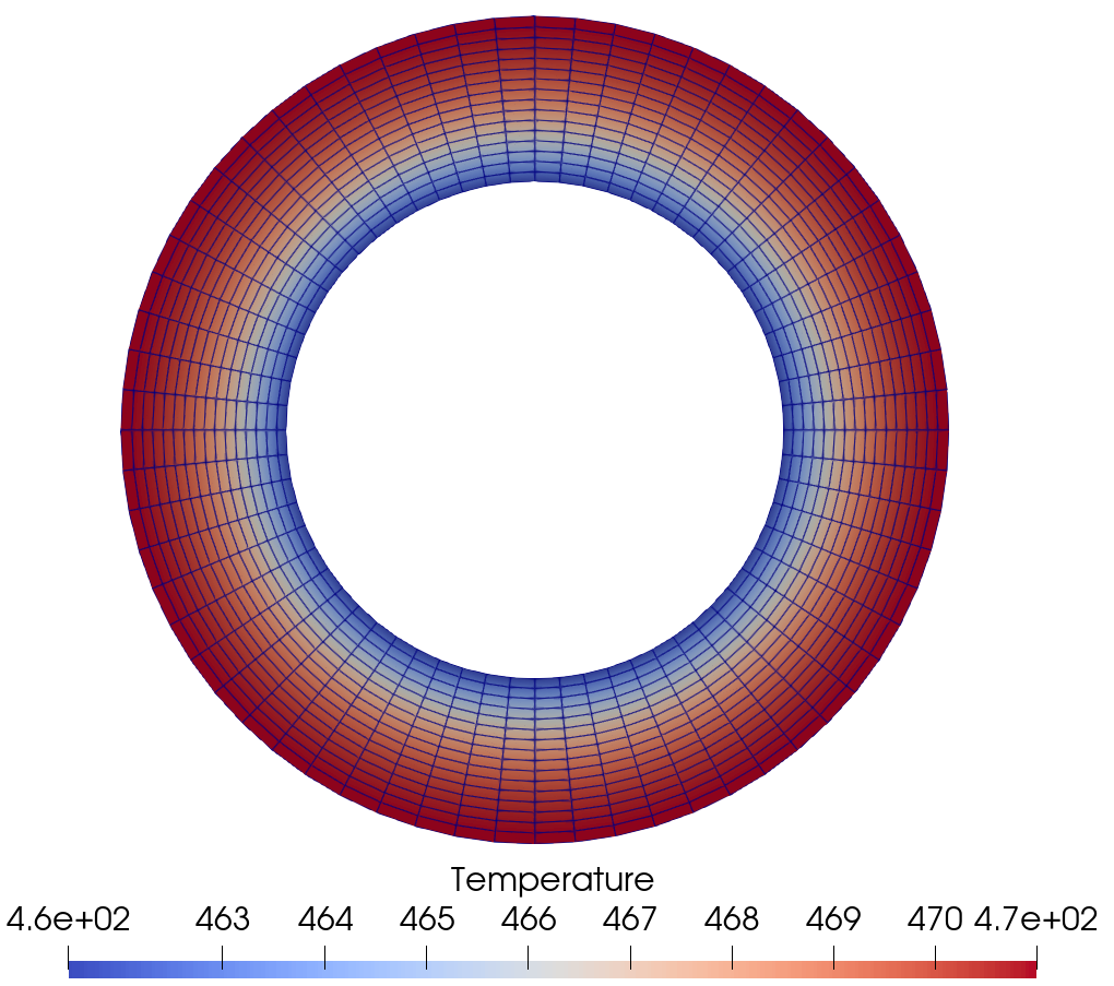
Figure 1: Initial annulus temperature profile
After optimizing the design to decrease the maximum temperature, the new design has a maximum temperature of around 160. Moreover, the volume constraint was satisfied to the given tolerance. The optimized inner and outer radii are now 1.199 and 8.075, respectively.
Figure 2 shows the optimized designs and the new temperature profile.
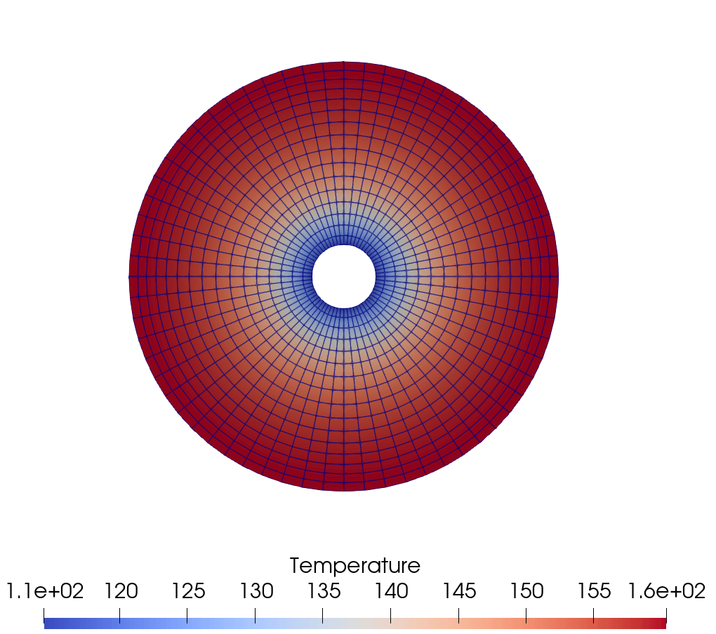
Figure 2: Optimized Annulus temperature profile