Material Inversion Example: Nonlinear Diffusion Reaction
The following illustrates the capability of the MOOSE Optimization module by applying the module to a nonlinear, material-inversion optimization problem:
where is the number of measurement locations and and are the simulated and measured state variables (e.g. temperature and displacement fields), respectively, at location . The parameter being optimized is the spatially dependent reaction rate (). The domain is meshed using a grid of quadrilateral elements, and time is discretized using implict Euler over ten uniform time steps. The measurement data is generated by evaluating the PDE with and sampling the resulting solution at 22 locations—shown in top left plot of Figure 1—at every time step, resulting in .
The reaction rate is parameterized using the mesh shown in the top right plot of Figure 1, where parameter values set the reaction rate at the 19 nodes and linearly interpolating between them. The initial condition for the optimization sets , emulating a diffusion-only system. TAO's bounded quasi-Newton line search (TAOBQNLS) was the chosen optimization algorithm. The following listings show the optimization input driving the optimization solve and the physics sub-application input used to calculate the forward and adjoint simulations.
Listing 1: Optimization input
[Optimization]
[]

[OptimizationReporter]
  type = ParameterMeshOptimization
  objective_name = objective_value
  parameter_names = 'reaction_rate'
  parameter_meshes = 'parameter_mesh_out.e'

  initial_condition = 0
  lower_bounds = 0

[]

[Reporters]
  [main]
    type = OptimizationData
    measurement_file = forward_exact_csv_sample_0011.csv
    file_xcoord = measurement_xcoord
    file_ycoord = measurement_ycoord
    file_zcoord = measurement_zcoord
    file_time = measurement_time
    file_value = simulation_values
  []
[]

[MultiApps]
  [forward]
    type = FullSolveMultiApp
    input_files = forward_and_adjoint.i
    execute_on = FORWARD
  []
[]

[Transfers]
  [to_forward]
    type = MultiAppReporterTransfer
    to_multi_app = forward
    from_reporters = 'main/measurement_xcoord
                      main/measurement_ycoord
                      main/measurement_zcoord
                      main/measurement_time
                      main/measurement_values
                      OptimizationReporter/reaction_rate'
    to_reporters = 'data/measurement_xcoord
                    data/measurement_ycoord
                    data/measurement_zcoord
                    data/measurement_time
                    data/measurement_values
                    params/reaction_rate'
  []
  [from_forward]
    type = MultiAppReporterTransfer
    from_multi_app = forward
    from_reporters = 'adjoint/inner_product data/objective_value'
    to_reporters = 'OptimizationReporter/grad_reaction_rate OptimizationReporter/objective_value'
  []
[]

[Reporters]
  [optInfo]
    type = OptimizationInfo
    items = 'current_iterate function_value gnorm'
  []
[]

[Executioner]
  type = Optimize
  tao_solver = taobqnls
  petsc_options_iname = '-tao_gttol -tao_max_it'
  #petsc_options_value = '1e-5 100' #use this to get results for paper
  petsc_options_value = '1e-5 5'
  solve_on = 'NONE'
  verbose = true
[]
[Outputs]
  csv = true
[]
Listing 2: Physics sub-application
[Mesh]
  [square]
    type = GeneratedMeshGenerator
    dim = 2
    nx = 16
    ny = 16
    xmin = 0
    xmax = 1
    ymin = 0
    ymax = 1
  []
[]

[Variables/u]
[]

[Reporters]
  [params]
    type = ConstantReporter
    real_vector_names = 'reaction_rate'
    real_vector_values = '0 0 0 0 0 0 0 0 0 0 0 0 0 0 0 0 0 0 0' # Dummy
    outputs = none
  []
  [data]
    type = OptimizationData
    variable = u
    objective_name = objective_value
    measurement_file = forward_exact_csv_sample_0011.csv
    file_xcoord = measurement_xcoord
    file_ycoord = measurement_ycoord
    file_zcoord = measurement_zcoord
    file_time = measurement_time
    file_value = simulation_values
    outputs = none
  []
[]

[Functions]
  [rxn_func]
    type = ParameterMeshFunction
    exodus_mesh = parameter_mesh_out.e
    parameter_name = params/reaction_rate
  []
[]

[Materials]
  [ad_dc_prop]
    type = ADParsedMaterial
    expression = '1 + u'
    coupled_variables = 'u'
    property_name = dc_prop
  []
  [ad_rxn_prop]
    type = ADGenericFunctionMaterial
    prop_values = 'rxn_func'
    prop_names = rxn_prop
  []
  #ADMatReaction includes a negative sign in residual evaluation, so we need to
  #reverse this with a negative reaction rate. However, we wanted the parameter
  #to remain positive, which is why there is one object to evaluate function
  #and another to flip it's sign for the kernel
  [ad_neg_rxn_prop]
    type = ADParsedMaterial
    expression = '-rxn_prop'
    material_property_names = 'rxn_prop'
    property_name = 'neg_rxn_prop'
  []
[]

[Kernels]
  [udot]
    type = ADTimeDerivative
    variable = u
  []
  [diff]
    type = ADMatDiffusion
    variable = u
    diffusivity = dc_prop
  []
  [reaction]
    type = ADMatReaction
    variable = u
    reaction_rate = neg_rxn_prop
  []
  [src]
    type = ADBodyForce
    variable = u
    value = 1
  []
[]

[BCs]
  [dirichlet]
    type = DirichletBC
    variable = u
    boundary = 'left bottom'
    value = 0
  []
[]

[Executioner]
  type = TransientAndAdjoint
  forward_system = nl0
  adjoint_system = adjoint
  petsc_options_iname = '-pc_type'
  petsc_options_value = 'lu'
  dt = 0.1
  end_time = 1

  nl_rel_tol = 1e-12
[]

[Problem]
  nl_sys_names = 'nl0 adjoint'
  kernel_coverage_check = false
  skip_nl_system_check = true
[]

[Variables]
  [u_adjoint]
    initial_condition = 0
    solver_sys = adjoint
    outputs = none
  []
[]

[DiracKernels]
  [misfit]
    type = ReporterTimePointSource
    variable = u_adjoint
    value_name = data/misfit_values
    x_coord_name = data/measurement_xcoord
    y_coord_name = data/measurement_ycoord
    z_coord_name = data/measurement_zcoord
    time_name = data/measurement_time
  []
[]

[VectorPostprocessors]
  [adjoint]
    type = ElementOptimizationReactionFunctionInnerProduct
    variable = u_adjoint
    forward_variable = u
    function = rxn_func
    execute_on = ADJOINT_TIMESTEP_END
    outputs = none
  []
[]

[AuxVariables]
  [reaction_rate]
  []
[]

[AuxKernels]
  [reaction_rate_aux]
    type = FunctionAux
    variable = reaction_rate
    function = rxn_func
    execute_on = TIMESTEP_END
  []
[]

[Postprocessors]
  [u1]
    type = PointValue
    variable = u
    point = '0.25 0.25 0'
  []
  [u2]
    type = PointValue
    variable = u
    point = '0.75 0.75 0'
  []
  [u3]
    type = PointValue
    variable = u
    point = '1 1 0'
  []
[]

[Outputs]
  exodus = true
  console = false
  csv = true
[]
The top right figure in Figure 1 shows the rate found from the optimization process. Figure 2 shows how close the solution from the optimized reaction rate is from the synthetic measurement data. The diffusion-only initial guess is shown by the square data points.
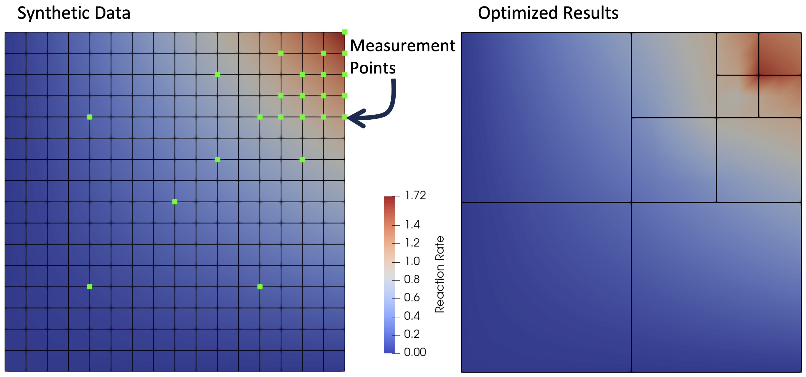
Figure 1: Left: Exact reaction rate, simulation mesh, and measurement locations. Right: Optimized rection rate and parameter mesh.
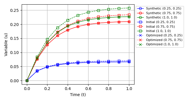
Figure 2: Comparing simulated transient solution with exact, initial optimization guess, and optimized reaction rate at several measurement locations (measurement and optimized data are visually identical).