Problem statement

This problem considers a coupled systems of equations on a 3-D domain : find and such that

where on the top boundary and and on the bottom boundary. The remaining boundaries are natural boundaries:

The domain, , is the same as utilized in Example 2. The weak form of this equation, in inner-product notation, is given by:

where are the test functions and and are the finite element solutions.

Create Convection Kernel

The convection component of the problem requires Kernel object just as described in Example 2 with one small addition - the Kernel will utilize a coupled variable rather than a known constant. "ExampleConvection.h" needs one new member variable to store the gradient of the coupled variable:

private:
  const VariableGradient & _grad_some_variable;

The source file "ExampleConvection.C" also includes a new parameter that defines the variable to couple into its kernel. Additionally, the computeQpResidual and computeQpJacobian functions in the source file now utilize the coupled value to compute the desired residuals and jacobians respectively:

#include "ExampleConvection.h"

// Don't forget to register your object with MOOSE
registerMooseObject("ExampleApp", ExampleConvection);

InputParameters
ExampleConvection::validParams()
{
  InputParameters params = Kernel::validParams();

  // Here we specify a new parameter for our kernel allowing users to indicate which other
  // variable they want to be coupled into this kernel from an input file.
  params.addRequiredCoupledVar(
      "some_variable", "The gradient of this variable will be used as the velocity vector.");

  return params;
}

ExampleConvection::ExampleConvection(const InputParameters & parameters)
  : Kernel(parameters),
    // using the user-specified name for the coupled variable, retrieve and store a reference to the
    // coupled variable.
    _grad_some_variable(coupledGradient("some_variable"))
{
}

Real
ExampleConvection::computeQpResidual()
{
  // Implement the weak form equations using the coupled variable instead of the constant
  // parameter 'velocity' used in example 2.
  return _test[_i][_qp] * (_grad_some_variable[_qp] * _grad_u[_qp]);
}

Real
ExampleConvection::computeQpJacobian()
{
  // Implement the Jacobian using the coupled variable instead of the 'velocity'
  // constant parameter used in example 2.
  return _test[_i][_qp] * (_grad_some_variable[_qp] * _grad_phi[_j][_qp]);
}

Input File Syntax

First, the mesh is defined by loading a file "mug.e".

[Mesh]
  file = mug.e
[]

Then, the two variables are defined: "diffused" and "convected", which refer to and from the problem statement, respectively. Both variables in this case are assigned to utilize linear Lagrange shape functions, but they could each use different shape functions and/or orders.

[Variables]
  [./convected]
    order = FIRST
    family = LAGRANGE
  [../]

  [./diffused]
    order = FIRST
    family = LAGRANGE
  [../]
[]

The problem requires three Kernels, two Diffusion Kernels, one for each of the variables and the ExampleConvection Kernel created above. It is important to point out that for the two Diffusion terms, the same code is utilized; two instances of the C++ object are created to application of the code to two variables. Additionally, the actual coupling of the equations takes place in the ExampleConvection object. The some_variable input parameter was created in the ExampleConvection Kernel and here is assigned to utilize the diffused variable.

[Kernels]
  [./diff_convected]
    type = Diffusion
    variable = convected
  [../]

  [./conv]
    type = ExampleConvection
    variable = convected

    # Couple a variable into the convection kernel using local_name = simulationg_name syntax
    some_variable = diffused
  [../]

  [./diff_diffused]
    type = Diffusion
    variable = diffused
  [../]
[]

For the given problem, each of the variables has a DirichletBC applied at the top and bottom. This is done in the input file as follows.

[BCs]
  [./bottom_convected]
    type = DirichletBC
    variable = convected
    boundary = 'bottom'
    value = 1
  [../]

  [./top_convected]
    type = DirichletBC
    variable = convected
    boundary = 'top'
    value = 0
  [../]

  [./bottom_diffused]
    type = DirichletBC
    variable = diffused
    boundary = 'bottom'
    value = 2
  [../]

  [./top_diffused]
    type = DirichletBC
    variable = diffused
    boundary = 'top'
    value = 0
  [../]
[]

Finally, the Executioner block is setup for solving the problem an the Outputs are set for viewing the results.

[Executioner]
  type = Steady
  solve_type = 'PJFNK'
[]

[Outputs]
  execute_on = 'timestep_end'
  exodus = true
[]

Running the Problem

This example may be run using Peacock or by running the following commands form the command line.

cd ~/projects/moose/examples/ex03_coupling
make -j8
./ex03-opt -i ex03.i

This will generate the results file, out.e, as shown in Figure 1 and 2. This file may be viewed using Peacock or an external application that supports the Exodus format (e.g., Paraview).

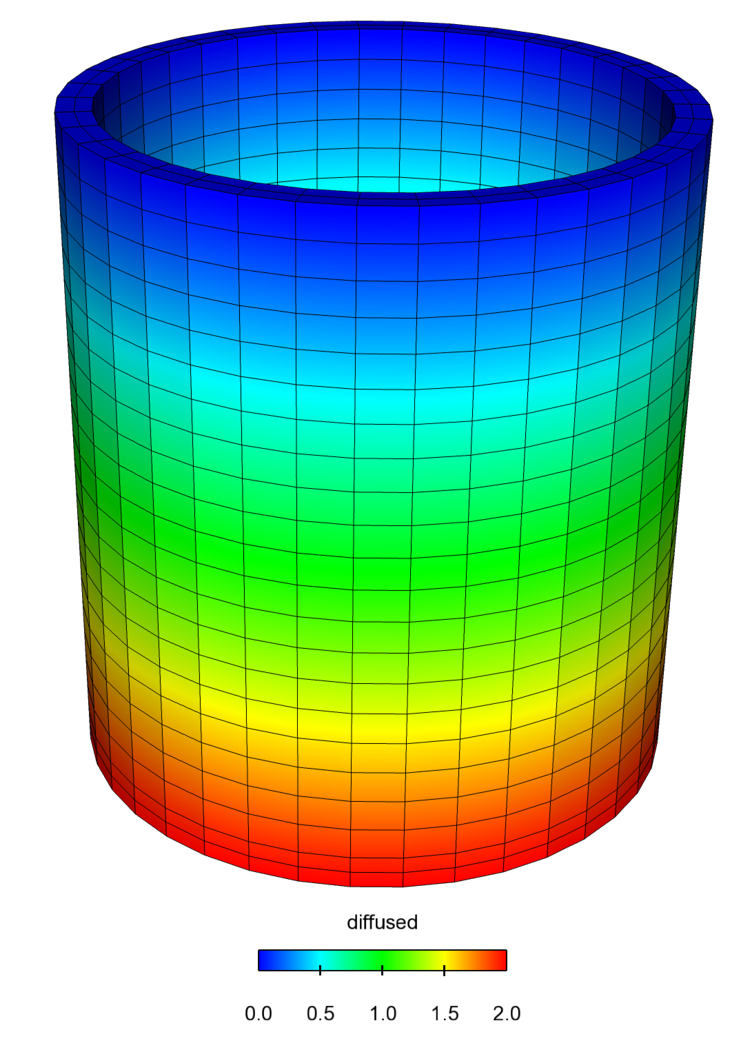
Figure 1: example 3 Results, "diffused variable"

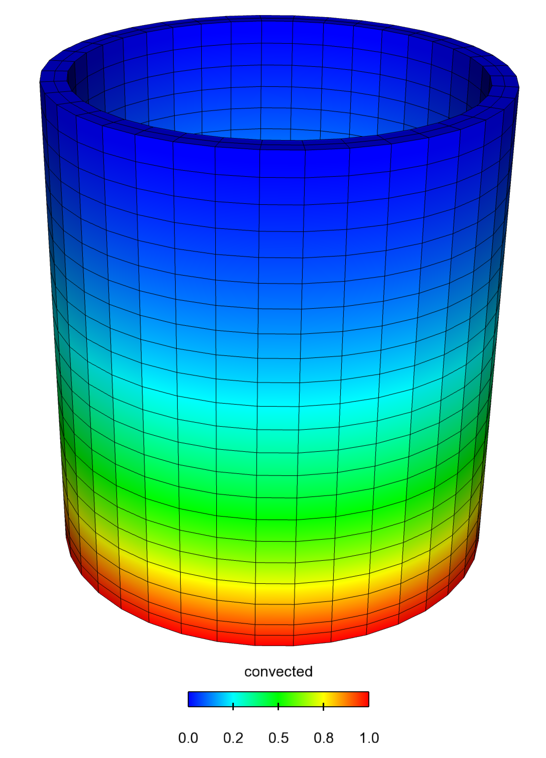
Figure 2: example 3 Results, "convected variable"

Complete Source Files

• (examples/ex03_coupling/ex03.i)

• (examples/ex03_coupling/include/kernels/ExampleConvection.h)

• (examples/ex03_coupling/src/kernels/ExampleConvection.C)

• (examples/ex03_coupling/src/base/ExampleApp.C)